Abstract
In this work, we propose considering the information from a polyphony for multi-pitch estimation (MPE) in piano music recordings. To that aim, we propose a method for local polyphony estimation (LPE), which is based on convolutional neural networks (CNNs) trained in a supervised fashion to explicitly predict the degree of polyphony. We investigate two feature representations as inputs to our method, in particular, the Constant-Q Transform (CQT) and its recent extension Folded-CQT (F-CQT). To evaluate the performance of our method, we conduct a series of experiments on real and synthetic piano recordings based on the MIDI Aligned Piano Sounds (MAPS) and the Saarland Music Data (SMD) datasets. We compare our approaches with a state-of-the art piano transcription method by informing said method with the LPE knowledge in a postprocessing stage. The experimental results suggest that using explicit LPE information can refine MPE predictions. Furthermore, it is shown that, on average, the CQT representation is preferred over F-CQT for LPE.
1. Introduction
Early approaches to solving tasks related to the research field of music information retrieval (MIR) relied on using music expert knowledge and hand-crafted features []. In recent years, a drastic shift in focus from hand-crafted features to data-driven approaches can be observed []. Specifically, deep neural networks (DNNs) trained in a supervised fashion have shown state-of-the-art results in various MIR tasks such as music source separation [,], instrument recognition [,], chord detection [], piano transcription [], and fundamental frequency estimation [].
One particular objective that has received less attention is local polyphony estimation (LPE) in music recordings. The task of LPE is to (locally) determine the degree of polyphony, i.e., the number of concurrently played musical notes at any given time within a music signal. LPE can either be inferred in an indirect manner (implicitly) by counting the number of simultaneously active notes estimated using a multi-pitch estimation (MPE) algorithm [,], or inferred explicitly, i.e., estimated directly from a music recording. For example, a DNN for MPE [] can be considered an implicit LPE method since (local) polyphony can be estimated as a side product of the method’s corresponding estimates. However, the DNN is tailored towards the task of MPE, aiming to determine the correct fundamental frequency of detected notes, and LPE plays a less significant role. The importance of polyphony information is disregarded [,].
In related literature, both implicit and explicit methods for LPE have been rarely investigated, especially for their importance in informing other MIR-related tasks in supervised scenarios. One exception is [], where an approach to explicit LPE is presented, which also uses that information to obtain better results from music instrument recognition. Nonetheless, explicit LPE remains a largely unexplored research direction for deep learning in MIR. The output of LPE is an additional, potentially useful side information that can reinforce many existing MIR and audio signal processing tasks. For example, instrument recognition [], music transcription [], and chord detection [] could benefit from LPE information. In these tasks, musical passages that contain an increased number of active notes, i.e., passages of high polyphony, are especially challenging examples of music transcription [], and information from LPE methods could help to focus on relevant pitches, increasing the overall prediction accuracy. Furthermore, LPE could be useful in training supervised music source separation approaches by introducing constraints, depending on the degree of polyphony, and thereby reinforcing neural networks for learning time-frequency masks for separation [].
In this study, we examine the decoupling of LPE from processing pipelines of existing MPE methods [,] and infer LPE directly from the analyzed music/audio recording. We aim to investigate whether data-driven approaches using convolutional neural networks (CNNs) can be employed to deliver robust methods for LPE and whether existing MPE models can improve their results using the information obtained from LPE. To do so, this study focuses on monotimbral piano recordings provided by the MIDI Aligned Piano Sounds (MAPS) dataset [] and the Saarland Music Data (SMD) []. This scenario allows us to perform an in-depth examination and comparison of various signal representations that are commonly used in MIR.
As for the contributions of this work, we (a) show that LPE information can improve MPE methods; (b) introduce a novel, synthetic dataset based on SMD, which mitigates the influence of note decays and the resulting mismatch between audio signals and note-level MIDI annotations; (c) propose a method for explicit LPE from classical piano recordings; and (d) systematically examine the Constant-Q Transform (CQT) and Folded-CQT as input signal representations for LPE.
The proposed method estimates the polyphony over short time segments (frames) of the music signal and is realized by means of CNNs that are trained in a supervised manner. We compare our proposed method for explicit LPE with a state-of-the art piano transcription method [] by applying the LPE information in a postprocessing stage on the results of said MPE method. Furthermore, we investigate the influence of music performance attributes, such as note decay, on LPE. MAPS and SMD are naturally affected by an imbalanced data distribution with respect to note pitches, degrees of polyphony, as well as composers.
The remainder of this manuscript is structured as follows: Section 2 gives an overview of related works. In Section 3, we describe the methodology behind the proposed method for LPE, including the models and feature representations. Section 4 provides information on the employed datasets of piano recordings and introduces the synthetic dataset. Section 5 elaborates on the persuaded experimental procedure for training and evaluating the proposed method. In Section 6, we present and discuss the results from the experimental procedure. Section 7 concludes this work by summarizing the findings of our study and by introducing plausible future research directions.
2. Related Work
The estimation of degrees of polyphony is closely tied with the detection of musical notes, i.e., automatic music transcription, which is a well-established task in the MIR community. The task of music transcription can also be seen as a way to perform MPE under the assumption that the transcribed notes correspond to the true set of pitches [,]. MPE algorithms estimate active pitches using multiple -estimation and a subsequent selection from multiple pitch candidates. Furthermore, the core idea of polyphony estimation extends to other research fields such as sound event detection [] and speaker recognition [] where, instead of musical notes, simultaneous sounds and voices need to be counted. Therefore, polyphony estimation is relevant for a broad variety of application scenarios ranging from music processing to machine listening, which are included in our literature review.
One of the earlier works aimed at music instrument recognition using LPE and MPE was presented in []. Specifically, an implicit method for LPE was presented and employs a set of cascaded comb filters to detect multiple pitches. The detected pitches are then used to estimate the degree of polyphony. Similarly, the work presented in [] proposed the use of filters inspired by the human auditory periphery to perform MPE for both polyphonic music and speech signals. Su et al. [] proposed to combine spectral information with temporal representations to refine the MPE for polyphonic music. More recent methods for MPE propose the use of modified wavelet transform to improve the overall performance in polyphonic music []. These are scenarios where explicit LPE could prove helpful, as it may help by providing a search scope and an upper boundary during musical sections with strong spectral overlap of the instruments and notes.
The works in this paragraph are purely centered around MPE. We believe they could benefit from incorporating explicit local polyphony information, which is why we list them here. In relation to music transcription, in [], it was proposed to perform MPE from harmonic envelopes of music signals, with the resulting pitch estimates used for polyphonic music transcription. Bohac et al. [] proposed an algorithm to first perform an identification of pitch/note candidates on a magnitude spectrum and to then perform a subsequent polyphonic music transcription. Furthermore, supervised learning and (deep) neural networks were proposed for the task of piano transcription in [].
Our work shares many commonalities with the following works. Specifically, it is similar to [], where the problem—applied to the “cocktail party” scenario with several speakers—was formulated as count estimation and discussed on the level of classification vs. regression. The authors implemented a bidirectional long short-term memory recurrent neural network (BLSTM-RNN) and suggested the use of CNNs. For our work, we assume the position of a classification problem. More related to MIR, the work presented in [] proposed an MPE method that highlights the importance of LPE, using a polyphony inference algorithm to determine the multiple pitches. Similarly in [], polyphony estimation was defined as a subproblem of MPE, for which a maximum likelihood approach was used to iteratively estimate fundamental frequencies. A polyphony estimate was then inferred by employing a threshold for the likelihood improvement. The corresponding results revealed that, for a polyphony of more than 5 notes, the estimation performance heavily deteriorates.
Kareer et al. [] proposed a supervised learning method for explicit LPE, which reinforces the subsequent task of musical instrument recognition. The authors created two simple CNNs, one initially optimized for LPE up to a polyphony degree of 4 and another for musical instrument recognition. The information from the LPE–CNN was used to transfer its domain knowledge to the task of instrument recognition. The results were compared to the MPE method from [] and showed better performance for the CNN-based method. This indicates that tackling polyphony estimation as a separate task can elevate the performance of subsequent related music processing tasks, i.e., music instrument recognition.
3. Methodology
Our proposed method first estimates the local degree of polyphony from a given music recording on a frame-level and then employs the polyphony information as a postprocessing step to improve the prediction quality of a multi-pitch estimation algorithm. To do so, we first computed two-dimensional and three-dimensional feature representations of time-domain audio signals as described in detail in Section 3.1. These features were given as input to a DNN, detailed in Section 3.2, which estimates the local degree of polyphony in each time frame. The DNN was initially trained in a supervised fashion and evaluated using labeled data taken from the MAPS configuration 2 and SMD-synth datasets, which are described in Section 4.
3.1. Feature Representations
We examined three feature representations that were given as input to our proposed method. Two of the representations were based on the constant-Q transform (CQT) [] and were denoted as the high-resolution CQT and the low-resolution CQT. The third representation was the recently proposed folded CQT []. The details for each representation are given in the following subsections, and an overview is given in Table 1. Prior to computation of the representations, all audio files were converted to monaural signals and all representations were based on time-frequency decomposition methods using a hop size of 512 samples. For audio processing and feature extraction, we utilized the librosa [] Python library (version 0.8.0, https://doi.org/10.5281/zenodo.3955228, accessed on 30 March 2021).

Table 1.
Overview of the feature representation properties. Note that batch normalization is performed in the input layer of all models.
3.1.1. High-Resolution Constant-Q Transform (HR-CQT)
HR-CQT was computed using a resolution of 36 bins per octave (three bins per semitone) and a sample rate of 44.1 kHz. After computing its magnitude spectrogram, we segmented the representation to equal-sized patches of five frames. We referred to this feature representation as “high-resolution” to distinguish it from the other feature representation, explained in the next subsection. No normalization took place at any point in this stage, similar to []. The analysis parameters for HR-CQT, i.e., minimum and maximum frequencies and bins per octave, were based on the MPE experiments on the MAPS dataset reported by Sigtia et al. [] and the available labels for the piano pitch range, which are explained in full detail in Section 5.1.
3.1.2. Low-Resolution Constant-Q Transform (LR-CQT)
In comparison to HR-CQT, the LR-CQT feature representation uses analysis parameters that lead to a reduced frequency resolution, and therefore, we refer to it as “low-resolution”. For LR-CQT, each audio file was downsampled to 22.05 kHz and then normalized by dividing the audio samples by the maximum absolute value []. Then, the CQT was computed over the same pitch range as the HR-CQT but with a reduced resolution of 12 bins per octave (one bin per semitone). Finally, we applied log-magnitude compression on the CQT features.
3.1.3. Folded CQT (F-CQT)
As illustrated in Figure 1, F-CQT [] represents a CQT frame of magnitude information as a matrix, i.e., a representation in two dimensions. To do so, the LR-CQT feature representation was first computed and, then, all bins in a given frame (left and middle subplot) were rearranged according to the circle of fifths, with the pitch classes re-ordered to C, G, D, A, E, B, and so forth. In a second step, the two lowest octaves were placed on top of each other. This constituted one row of the F-CQT matrix. For the next row—here, the second dimension came into effect—the highest octave from the previous row and the next octave were stacked alongside each other, as shown in the right subplot of Figure 1. As a result, harmonics related to the same fundamental frequency remained in close proximity. This allowed small convolutional kernels to easily capture harmonic overtone patterns of musical notes, which usually span several octaves. To summarize, in contrast to the two-dimensional LR-CQT and HR-CQT features, the F-CQT feature representation became three-dimensional including the time-axis, which needed to be considered in the CNN architecture explained below.
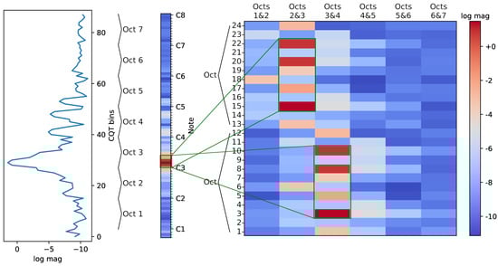
Figure 1.
One-dimensional and two-dimensional log-magnitude (log mag) representations of a Constant-Q Transform (CQT) frame of a synthetic tone with the pitch D3: 1D CQT frame (left and middle) and 2D F-CQT feature (right). Corresponding pitch ranges in both representations are shown by green rectangles. Notice the zig-zag octave ordering in the Folded-CQT (F-CQT).
3.2. CNN Models
In this work, we examined the CNN-based MPE model proposed by Kelz et al. [] as a baseline model (denoted as ConvNet-MPE). The task of LPE, however, was performed using several CNN models specifically tailored towards the feature representations introduced in Section 3.1. These models mainly differ in kernel shapes and pooling layers. All model types are summarized in Table 2 and will be detailed in the next sections.
Table 2.
Overview of all neural network model architectures with the respective task, feature representation, kernel shapes of the first convolutional block, number of classes, as well as number of model parameters.
MPE Model: ConvNet-MPE
The baseline for all comparisons forms the “ConvNet” architecture used for MPE as proposed by Kelz et al. in []. The MPE results reported in Section 6 show that our reimplementation achieved similar results, as reported in the original paper. The ConvNet-MPE consists of three convolutional blocks (CB), each one including a convolutional layer, batch normalization, rectified linear unit (ReLU) activation, and dropout. The dropout was applicable only during training. The first two CBs both had 32 filters with a (3, 3) kernel size and a momentum-based batch normalization. The momentum was set to 0.1. No zero-padding took place between the convolutional operations (“valid padding”). This pair of CBs was followed by a max-pooling layer with a pool size of (1, 2) and a dropout layer with a small dropout of 0.25. With 64 filters, the last CB had a larger number of filters and it used a smaller kernel size of (1, 3). After the three CBs, two dense layers were used with 512 and 88 units, respectively. The sigmoid activation function was used at this stage. Furthermore, dropout between the two dense layers was used, with a probability of 0.5. All the computational layers in this model do not contain any bias terms. The ConvNet-MPE was trained using HR-CQT and minimizing the binary crossentropy loss function.
3.3. LPE Models
All models for LPE are illustrated in Figure 2. It can be seen that all of the investigated LPE models, with the exception of the ConvNet-LPE, are extensions of the same baseline architecture. They have a batch normalization (BN) at the input stage, three CBs, the same number of filters per CB, and the final stack of dense layers in common.
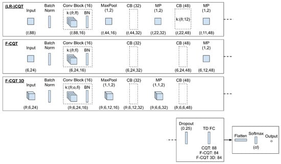
Figure 2.
Overview of three convolutional neural network (CNN) architectures created for the local polyphony estimation (LPE) experiments. The output tensor shapes are given underneath each layer. Abbreviations: = classes, = fifths, = frames, = features, k = kernel, o = octaves, and t = time. Detailed parameter values are described in Section 3 and Section 5.
Each CB consists of a convolutional layer for which the output is passed through a BN and a rectified linear unit (ReLU) activation function. After the last CB, dropout was applied with a probability of 0.25. Then, a bias-free fully connected (FC) layer was used with as many units as bins in the original feature representation and with a tanh activation function. This FC was followed by another FC with Softmax activation and as many units as the current polyphony scenario (see Section 5.2). All CBs used same-padding and default stride sizes of (1, 1). Finally, all LPE models (again, with the exception of the ConvNet-LPE) were trained using the categorical cross-entropy loss function.
3.3.1. ConvNet-LPE
By simply changing the number of units at the output layer of the ConvNet-MPE to 3, 6, or 13 units and by using a softmax activation function (as described in Section 4), we could effectively shift the purpose of the model and apply it to the task of LPE. This allowed us to observe whether the general ConvNet architecture was suitable for LPE. The optimizer and learning rate configuration as well as the input feature representation remained identical to the ConvNet-MPE.
3.3.2. CQT Model
The CQT model took portions of a CQTgram as input as determined by the batch size. For this model, these portions could be either from the LR-CQTgram or HR-CQTgram, which had feature dimensions at sizes of 88 or 264, respectively. For the first two CBs, we chose a kernel size of , where is the number of frames it spans and is the number of neighboring CQT-features (bins). Sizes of 12 (one full octave) and 24 bins (two full octaves) were chosen to allow the kernel to cover a similar amount of notes as the F-CQT to investigate the influence of their differences. The pooling layers downsampled information from the feature dimension step-by-step. This required us to adjust the kernel in the last CB to a fixed 12 bins to prevent excessive padding and to reduce the number of parameters.
3.3.3. F-CQT Model
The F-CQT model took individual F-CQT frames as input. Due to the arrangement of the F-CQT, each frame had a two-dimensional shape: with 12 bins per octave and 7 octaves, the shape of one frame was 6 × 24. Therefore, the kernel size in the first CB was of the form , with o denoting the number of octaves and denoting the number of fifths. In [], a size of (4, 3) was proposed, as this kernel size can span 4 octaves and 3 fifths. In general, an F-CQT convolutional kernel has the advantage of covering harmonics within an octave with less parameters. Due to the reduced kernel sizes in F-CQT over CQT and the resulting lower number of model parameters, we waived all intermediate pooling steps after each CB except for the final max-pooling over the tensor dimension associated to the fifths.
3.3.4. F-CQT 3D Model
The F-CQT 3D model has a similar architecture as the F-CQT model. In contrast to the F-CQT model, the F-CQT 3D model incorporates temporal context similar to the CQT model if its convolution kernels span several frames. As input to the F-CQT 3D model, we concatenated multiple consecutive F-CQT frames and obtained a three-dimensional input feature. A 3D-kernel of the form then scanned the input in the CBs. Since this procedure potentially leads to a much larger amount of parameters, we shrank the feature representation during the forward pass: Pooling layers were applied along one row of octaves—which equals the dimension of fifths—after the first and second CB.
4. Datasets
4.1. MIDI Aligned Piano Sounds (MAPS) Dataset
The MAPS dataset was published by Emiya et al. [] and consists of 4 categories of piano sounds, including isolated notes, chords, and full pieces of music. The dataset content covers a large variety of recording conditions. For our investigations, we focused on the classical music pieces with a total file count of 270. A subset of them (210 files) was originally synthesized directly from MIDI files with realistic piano sound banks, and another subset (60 files) was recorded using a Disklavier, which automatically transcribes the played notes during a performance into MIDI data.
For the preliminary study of the performance of a multi-pitch estimation model, we evaluated the ConvNet architecture, which achieved state-of-the-art results on a particular variant of this subset of the MAPS dataset. This variant is referred to as “MAPS configuration 2” and was first investigated by Sigtia et al. [], although the exact splits were not published. In [], the authors provided the means to recreate their own splits. For the sake of generalization, we built upon our own training and validation file lists and recreated MAPS configuration 2: We used any synthesized classical music material as training and validation sets, such that the test set only comprises the 60 real Disklavier recordings. The remaining 210 files were split randomly into the training and validation subsets using the original ratio of 180/30 files.
4.2. Saarland Music Data (SMD)
We also considered the SMD MIDI-Audio Piano Music subset of the Saarland Music Data []. It consists of 50 polyphonic classical piano recordings (monotimbral) of different composers, which range from Bach over Liszt to Mozart. Several interpreters have recorded this set in a controlled environment using a Disklavier to record the performance simultaneously as audio and MIDI format in a similar fashion to the MAPS dataset.
The dataset contains approx. 4 h and 43 min of piano music. Some composers are overrepresented relative to others, for instance, Bach with 8 files and 18.25 min, Beethoven with 7 files and 50.75 min, and Chopin with 13 files and 51.35 min. These three composers make up almost half of the dataset. This circumstance raises some thought towards the most practicable split strategy, and there are several strategies to tackle this, e.g., using data augmentation, not utilizing a validation set, or using a composer-level dataset split. We split SMD into training, validation, and test sets using a 70/14/16 percentage ratio. The only constraints for this splitting method are that the maximum polyphony of 12 notes for this dataset must at least exist within the annotations of both the train and test sets.
4.3. SMD-Synth
SMD-synth is a derivation and further development of the SMD dataset. It was created by resynthesizing the SMD MIDI files using a realistic piano sound bank (Standard NN-XT soundbank “B Greatpiano 1.0”, Reason digital audio workstation (DAW)), for which the characteristic sound parameters such as sustain, note decay, and release have been completely disabled for note-off events. In effect, this results in piano notes being cut off the instant a note-off event occurs. In the following, we describe the line of thought that led to the creation of this dataset.
In real-world scenarios, when a piano note is released, it is not immediately damped; it sustains a reverberation and resonance for a certain amount of time depending on the piano’s nature of construction. This behavior and the usage of the sustain pedal cause major problems for polyphony estimation: Whenever a piano key is released, the MIDI processor generates a note-off event, even though the sound that the key produced is still audible and recorded. This introduces unwanted label noise with respect to local polyphony annotations, as labels are missing to accurately represent the magnitude information of the feature representation. With SMD-synth, we aimed to alleviate this by practically removing these after effects: the labels thus strictly reflect the actual notes played and therefore match the MIDI observations to the expected amplitude information to a much greater extent. An example can be seen in Figure 3.
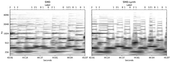
Figure 3.
Example of label noise. This figure shows two high-resolution (HR-)CQT spectrograms of the same musical piece excerpt contained in Saarland Music Data (SMD) (left) and SMD-synth (right). On top of each spectrogram, the frame-based degree of polyphony, i.e., the derived label from the MIDI information used for training, is displayed, which is equal for both. Each tick represents a change in the label. For SMD-synth, note that the gaps in the spectrogram are in correlation with no MIDI information (“0”), resulting in actual silence both in the annotations and magnitude information.
As an additional benefit, the synthetic dataset could be useful for future research studying perceptual and acoustic aspects of piano performances as well as for the evaluation of MPE algorithms, since the decay problem is also highly relevant in that area.
At the same time, the dataset was manually cleaned from obvious errors in MIDI events, which were either due to erroneous recognition of, for instance, very quickly or slightly pressed and released notes without actually producing sound or glitches in the MIDI processor. Score sheets were taken into account for that. This procedure may introduce new silence frames. Furthermore, the start and end of the recordings were trimmed closer to the first note onset and last note offset, removing some silence. As these corrections were carried out manually, a similar endeavour would have been infeasible for the MAPS configuration 2 dataset regarding time requirements.
The class distributions between SMD and SMD-synth changed mostly for silence (class 0). Note that, even though both distributions are very similar, the sound characteristics are very different. This foreshadows different results between the datasets due to the difference in distribution of the input spectrograms.
In conclusion, the SMD-synth dataset purposefully lacks the typical sound characteristics of a piano after a note is played but retains the musical aspect of the original compositions while minimizing the number of missing labels. This allows us to provide a more realistic environment for our study of LPE than a fully arbitrarily synthesized dataset. Last, but not least, it allows us to observe whether models trained this way can generalize onto real environments.
5. Experimental Procedure
5.1. Label Acquisition
In order to generate labels for LPE, we made use of the MIDI files that accompany the musical pieces from both datasets. The MIDI files contain the physical onset and offset time as well as the respective MIDI number for each note event, which corresponds to its pitch. We mapped these events to a fixed temporal grid in order to encode all musical notes as a binary matrix, which consists of the frame-wise pitch activity for 88 piano notes. The musical notes contain a pitch range of [21:108], covering 88 notes from A0 to C8. In the special case for the F-CQT feature representation, this range was limited to 84 notes within [24:107] (C1 to H7, 84 notes) to prevent zero-padding.
For the case of polyphony estimation, we determined the number of active pitches by summing over the 88 piano notes. This sum directly translates into the degree of polyphony d. Additionally, for the case of spectral patches that cover multiple time frames, the pitch label target is the center frame.
5.2. Class Partitioning Strategies
With the polyphony values for the datasets at hand, we defined each degree as its own class and calculated their distributions. The overall distributions are presented in Figure 4. As can be seen, the total number of frames with , and for SMD-synth even with account for less than of each dataset. In comparison to MAPS, SMD-synth also exhibits a much greater incidence of classes 0 and 1. These two classes correspond to silent frames and frames with just one active pitch.
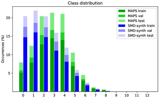
Figure 4.
Class distributions over MIDI Aligned Piano Sounds (MAPS) configuration 2 and SMD-synth datasets, with their respective subset splits. The highest available class is 12, which translates into “a polyphony degree of 12”—12 notes are active at the same time. The occurrences for classes higher than 5 diminish rapidly. Table 3 presents further insights into the subsets.
Due to this imbalance, we investigated three different class partition strategies for LPE. In the first strategy, we considered three classes: silence (0), monophony (1), and polyphony (2, more than one note active). Hence, we grouped all degrees of polyphony into class 2. In the second strategy (6 classes), we aimed to detect more specific degrees of polyphony. With regard to the imbalance for degrees of polyphony as stated above, we grouped all degrees into class 5. Then, classes 0 and 1 could be handled as before and the other classes 2–4 were specific examples of degrees of polyphony, where 2–4 notes were played simultaneously, respectively. Class 5 then combined all higher degrees again. As a third strategy, we considered all 13 degrees of polyphony, which resulted from the maximum polyphony of 12 in both datasets. With this third strategy, we aimed to observe where the largest drop in prediction performance appears.
5.3. Model Training and Evaluation
An overview of this experimental procedure is given in Figure 5. We started by training the ConvNet-MPE on the MAPS configuration 2 dataset and by computing MPE estimates from the test files. Since this is a binary classification task, the MPE predictions were thresholded into binary pitch activations using a value of 0.5. All the parameters of the ConvNet-MPE and ConvNet-LPE were randomly initialized with values drawn from a uniform distribution and scaled using the method presented in []. Stochastic gradient descent with a learning rate of 0.005 and a batch size of 1024 was used for optimizing the parameters of ConvNet-MPE. In addition to that, weight decay was used during optimization.
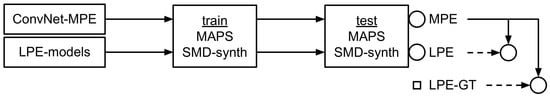
Figure 5.
Experimental procedure. The rows are to be viewed as separate evaluation paths. Circles are evaluation points. The ConvNet-multi-pitch estimation (MPE) model’s prediction values are manipulated in a postprocessing step by the local polyphony estimation (LPE) information coming from different sources. Each is evaluated separately to measure its influence on MPE, as described in Section 5.4.
The learning rate was halved every 5 epochs, and early stopping was used with a patience of 20 epochs. Apart from the learning rate, all of these choices followed the proposed hyperparameters presented in []. For the LPE models, with the exception of the ConvNet-LPE, the parameters were initialized randomly from a uniform distribution and scaled according to the method presented in []. Furthermore, Adam was used as an optimizer with a learning rate of . Similarly to the ConvNet-MPE model, an early stopping mechanism was used with a patience of 20 epochs. All models were trained with a maximum of 100 epochs, and we selected the models with the lowest validation loss during training for evaluation.
For both the LR-CQT and HR-CQT features, we systematically tested different patch sizes and kernel sizes in the first convolutional layers. LR-CQT in particular was subject to further parameter experiments, where the duration per spectral patch varied between 1, 3, and 5 frames to investigate the influence of temporal context size on the model performance, on top of varying kernel sizes.
For evaluating the models, we reported the micro-averaged precision, recall, and F1-score values using the scikit-learn [] Python library (version 0.23.2). The results for this were the baseline for successive experiments. Next, we trained the LPE models on the different class scenarios and computed frame-level LPE predictions. This was a multi-class task, and we reported both the F1-macro and F1-micro scores.
The LPE information was then used to refine the MPE predictions from these three different sources: (a) the ground truth, denoted as LPE-GT; (b) the ConvNet architecture itself (ConvNet-LPE); and (c) other LPE models—simple CNNs designed for the task of LPE and for different feature representations, where “simple” refers in this context to low complexity in terms of building blocks and trainable parameters. We expected source (a) to give us the best results and (b) to be close to the baseline, with (c) possibly exceeding (b) but generally remaining in the area between the baseline result and (a). See Section 5.4 for a description of this MPE refinement.
A full report of these experiments on MAPS configuration 2 is presented in Table A1. Table 4 and Table 5 have been reduced to the parameters that lead to the best results.
Table 4.
Experiments based on MAPS configuration 2, as described in Section 5 and Section 5.3. The abbreviations for model parameters are cl = classes, krnl = input kernel size (if applicable), fr = frames (if applicable); and for performance metrics: P = Precision, R = Recall, F = F1-score, M = macro-average, µ = micro-average, and Fµ = difference between baseline MPE and MPE informed by LPE. Grey highlighted cells refer to upper bound performance; bold-face refers to the highest observed performance.
Table 5.
Experiments based on SMD-synth, as described in Section 5 and Section 5.3. The abbreviations for model parameters are cl = classes, krnl = input kernel size (if applicable), fr = frames (if applicable); and for performance metrics: P = Precision, R = Recall, F = F1-score, M = macro-average, µ = micro-average, and Fµ = difference between baseline MPE and MPE informed by LPE. Grey highlighted cells refer to upper bound performance; bold-face refers to the highest observed performance.
In the final cross-dataset experiments utilizing both datasets that we presented, we evaluated the generalization capabilities of the MPE and LPE models on unseen data with very different sound characteristics to what they were trained with. For this, we chose the ConvNet-MPE, its LPE version and the best performing one from the other LPE models. In this cross-data experiment, we trained these models on one dataset and evaluated them on the test set of the other, and vice-versa.
It should be stated that, for all of the above-described experiments, we used the full piano recordings from the respective datasets. This differs from the evaluation procedure described in [,], where 30 second excerpts were used. Consequently, the reported results in Section 6 are expected to be different from the previously mentioned studies. However, using the whole music recordings provides a less biased evaluation procedure that reflects the generality of our results.
5.4. MPE Postprocessing
The processing of LPE information was conducted by means of a comparison where LPE was given priority over the MPE predictions. If the LPE for a frame predicted silence (class 0), then all sigmoid outputs from the MPE were set to zero. For all other classes, a ranking algorithm was engaged: The number of active notes as predicted by LPE was the criterion for final pitch activations. We illustrated this in the following with a few examples.
Instead of using a fixed decision threshold of in the MPE model, the degree of polyphony predicted by the LPE model was used for a ranking-based selection of the predicted pitches. For instance, if the LPE model predicted one active pitch, then the pitch with the highest sigmoid output value from the MPE model was chosen. If MPE predicted more active notes than the LPE, then the active pitches with the lowest confidences were ignored accordingly. If LPE gave the highest class in each scenario (except the 13-class scenario), it was checked whether the number of pitches predicted by the MPE model (a) surpassed this class, in which case nothing was done, or (b) fell behind this class, in which case as many notes as the LPE model predicted were activated according to the highest confidences.
In the case where the LPE information came from low-resolution feature representations, the number of audio frames was two times smaller than that for high-resolution features. This posed a problem for direct refinement of the MPE. To circumvent this, we upsampled the LPE frames by a factor of 2.
6. Results
Our first observation from Table 4 and Table 5 using the LPE ground truth confirms our hypothesis that LPE can be used as a postprocessing step to refine and improve MPE predictions. This is true for both datasets and all class scenarios. The margin for improvement decreases when the MPE model already provides very good prediction results, as for the case of SMD-synth, where the improvement using LPE for refinement is barely 2 percentage points in the micro-averaged F1-score.
It can also be seen there that this type of improvement grows higher as the polyphony class scenario becomes more difficult. This is an expected behavior, since higher degrees of polyphony are generally challenging for MPE. The confidences for lower degrees of polyphony, where the spectral information also appears less noisy, are higher, and thus, the room for improvement shrinks.
An interesting observation in this relation can be made from the micro-averaged precision and recall columns in the result Table 4 and Table 5 in comparison to the baseline: LPE can greatly improve recall, while some precision is usually lost. We assume this is because LPE is able to correct some false negatives, while due to computation of the micro-average, some of the precision (more false positives in relation) becomes lost—and it will reveal where MPE made wrong pitch predictions: LPE only pushes the results towards the right number of notes but does not correct incorrect pitch estimates.
The largest drop in performance occurs between the class scenarios 3 and 6. This is in correlation with previous findings of []. For all experiments, the F1-macro scores nearly halve as the class scenarios increase in difficulty, while the F1-micro scores for the 6-class and 13-class scenarios largely remain in the same area. Interestingly, the F1-micro scores for MAPS configuration 2 (Table 4) drastically drop by approximately 50 percentage points, whereas for SMD-synth (Table 5), the drop is approximately half of that. A similar observation can be made in the cross-data evaluation Table 6. In certain F-CQT configurations, the 13-class scenario can even slightly outperform 6 classes in the micro-averaged F1-score.
Table 6.
Results from the cross-data experiment as described in Section 5.3. The abbreviations for model parameters are cl = classes; and for performance metrics: P = Precision, R = Recall, F = F1-score, M = macro-average, µ = micro-average, and Fµ = difference between baseline MPE and MPE informed by LPE. Bold-face refers to the highest observed performance.
The F-CQT representation appears suitable for LPE: the F-CQT model in particular, which has the least parameters of all models (cf. Table 2), can compete with the CQT model using LR-CQT. The F-CQT 3D model appears more robust than the F-CQT model owing to the additional time-contextual information. For SMD-synth, both models perform equally. Seeing that the feature representations with higher resolutions are able to achieve considerably higher scores for the MPE task, we suggest creating a “high-resolution folded CQT (HR-F-CQT)” for future work as well.
The CQT model with an HR-CQT input feature representation performs best overall, closely tied with the ConvNet-LPE, which also uses HR-CQT. The CQT model has a considerably lower number of parameters (cf. Table 2). It should be noted though that, coupled with (3, 24) kernels, it takes up to 3× more computation time than the ConvNet-LPE with a (3, 3) kernel and 7× more compared to the F-CQT with a (4, 3) kernel. Kernels spanning 3 time frames appear to be the best compromise on average. We suspect that 5 time frames add too much noise to the kernels and that 1 time frame is simply not enough information. The same is true for the F-CQT 3D model. For the F-CQT representation in particular, kernels such as (4, 6) or (3, 4, 6) spanning the double number of per-octave bins perform slightly worse on average. All of this is true for the experiments on MAPS configuration 2 in Table 4 and Table A1 and on SMD-synth in Table 5.
Figure 6 demonstrates the generalization capability of the HR-CQT LPE-model, which achieved the best MPE refinement on average throughout the experiments. The percent-wise class distributions for the polyphony classes 2 and 3 are relatively similar between both datasets. However, a model trained on MAPS configuration 2 and evaluated on the SMD-synth test set performs worse for these classes than vice versa. This may be due to label noise and resulting mismatch with the magnitude information, as demonstrated in Figure 3, which has been greatly reduced in SMD-synth. Thus, a model trained on SMD-synth may be able to distinguish these classes better but then suffers in the recognition of the silence class. These problems can be attributed to the error sources mentioned above: silence is confused with monophony and some lower degrees of polyphony, which corresponds exactly to the label noise problem in MAPS configuration 2. In other words, if a model is trained with noisy labelled data, i.e., the silence mismatch illustrated in Figure 3, it can make wrong predictions between silence and the first degrees of polyphony. However, the mitigated label noise in the SMD-synth makes the model predictions more robust towards the detection of silence.
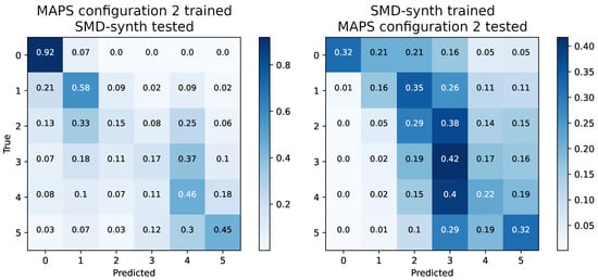
Figure 6.
Confusion matrices for a cross-data evaluation on the 6-class scenario, based on the LPE F1-micro of the CQT-model with HR-CQT input features and an input kernel size of (3, 24) spanning over 3 time frames of a patch with 5 time frames.
Generally, the LPE models need to be very well-adjusted to their task with respect to kernel sizes, general architecture, and input feature representation. Seeing that our proposed model architectures are considerably less heavy in terms of complexity than the ConvNet yet, in some cases, performing better, we deem that there is potential for more effective architectures that are able to refine MPE.
7. Conclusions
We proposed to decouple local polyphony estimation (LPE) from current multi-pitch estimation (MPE) methods to actively refine predictions of MPE methods. We tested the hypothesis that estimating LPE directly and feeding it into an MPE postprocessing step could improve the MPE predictions. We proposed a method to achieve that goal in a postprocessing stage. The results confirm that this approach has a potential to refine MPE, which is bound to several factors: the underlying feature representation and the parameters and architecture of the model. Nonetheless, the general method shown here to employ LPE information is applicable to any MPE model. Thus, we suggest that researchers should apply this method and test whether they can easily enhance their results.
For the future, LPE may hold more potential if it is directly integrated into pitch estimation models for joint LPE/MPE, i.e., as an additional input to an MPE model. This way, the number of active pitches coming from an LPE may serve as a search scope. The underlying MPE model may benefit from this as it could focus on finding the correct pitches for this search scope instead of all 88 notes. This could improve actual pitch predictions. For model generalization, domain adaptation could be a useful technique [].
Author Contributions
All three authors substantially contributed to this work, including the formalization of the problem, the development of the ideas, and the writing of this manuscript. M.T. implemented the approaches, handled the data curation, and conducted the experiments. All authors have read and agreed to the published version of the manuscript.
Funding
This work has been supported by the German Research Foundation (AB 675/2-1).
Data Availability Statement
The SMD-synth [] dataset, as described in Section 4.3, is publicly accessible under https://doi.org/10.5281/zenodo.4637908, accessed on 30 March 2021.
Conflicts of Interest
The authors declare no conflict of interest.
Appendix A
Table A1.
Experiments based on MAPS configuration 2, as described in Section 5 and Section 5.3. The abbreviations for the model parameters are cl = classes, krnl = input kernel size (if applicable), and fr = frames (if applicable) and for the performance metrics are P = precision, R = recall, F = F1-score, M = macro-average, µ = micro-average, and Fµ = difference between baseline MPE and MPE informed by LPE. Grey highlighted cells refer to upper bound performance; bold-face refers to the highest observed performance.
| LPE | MPE | ||||||||
|---|---|---|---|---|---|---|---|---|---|
| base model | cl | krnl | fr | FM | Fµ | Pµ | Rµ | Fµ | Fµ |
| ConvNet-MPE | 88 | (3, 3) | 3 (5) | n/a | n/a | 70.79 | 61.43 | 65.78 | n/a |
| base informed | |||||||||
| LPE-GT | 3 | - | - | 100.0 | 100.0 | 74.20 | 63.03 | 68.16 | +2.38 |
| 6 | - | - | 100.0 | 100.0 | 71.59 | 70.25 | 70.91 | +5.13 | |
| 13 | - | - | 100.0 | 100.0 | 71.25 | 71.25 | 71.25 | +5.47 | |
| ConvNet-LPE | 3 | (3, 3) | 3 (5) | 59.32 | 82.20 | 69.65 | 61.60 | 65.38 | −0.40 |
| 6 | (3, 3) | 3 (5) | 31.00 | 34.48 | 61.83 | 63.58 | 62.69 | −3.09 | |
| 13 | (3, 3) | 3 (5) | 14.30 | 32.58 | 65.01 | 59.38 | 62.07 | −3.71 | |
| HR-CQT | 3 | (1, 24) | 1 (5) | 56.95 | 80.46 | 69.65 | 60.47 | 64.73 | −1.05 |
| 6 | (1, 24) | 1 (5) | 30.34 | 33.11 | 59.12 | 67.40 | 62.99 | −2.79 | |
| 13 | (1, 24) | 1 (5) | 14.47 | 30.15 | 58.49 | 68.06 | 62.91 | −2.87 | |
| 3 | (3, 24) | 3 (5) | 59.12 | 83.93 | 68.80 | 62.85 | 65.69 | −0.09 | |
| 6 | (3, 24) | 3 (5) | 31.88 | 34.70 | 65.39 | 61.51 | 63.39 | −2.39 | |
| 13 | (3, 24) | 3 (5) | 13.55 | 32.85 | 62.90 | 63.43 | 63.16 | −2.62 | |
| 3 | (5, 24) | 5 | 60.39 | 81.60 | 69.83 | 61.26 | 65.26 | −0.52 | |
| 6 | (5, 24) | 5 | 31.27 | 36.15 | 66.32 | 60.22 | 63.12 | −2.66 | |
| 13 | (5, 24) | 5 | 13.95 | 32.33 | 61.33 | 64.88 | 63.06 | −2.72 | |
| LR-CQT | 3 | (3, 24) | 3 | 58.52 | 82.74 | 69.72 | 61.03 | 65.09 | −0.69 |
| 6 | (3, 24) | 3 | 28.32 | 34.25 | 63.72 | 60.12 | 61.87 | −3.91 | |
| 13 | (3, 24) | 3 | 12.98 | 33.30 | 65.88 | 55.53 | 60.26 | −5.52 | |
| F-CQT | 3 | (4, 3) | 1 | 49.16 | 79.21 | 68.65 | 59.82 | 63.93 | −1.85 |
| 3 | (4, 6) | 1 | 52.10 | 79.74 | 68.99 | 59.80 | 64.07 | −1.71 | |
| 6 | (4, 3) | 1 | 21.02 | 25.44 | 58.14 | 53.00 | 55.94 | −9.84 | |
| 13 | (4, 3) | 1 | 7.25 | 22.29 | 71.64 | 31.46 | 43.72 | −22.06 | |
| F-CQT 3D | 3 | (3, 4, 3) | 3 | 53.50 | 80.35 | 69.75 | 59.28 | 64.09 | −1.69 |
| 3 | (3, 4, 6) | 3 | 53.66 | 79.75 | 69.63 | 58.74 | 63.72 | −2.06 | |
| 6 | (3, 4, 3) | 3 | 27.14 | 33.19 | 64.99 | 55.15 | 59.67 | −6.11 | |
| 13 | (3, 4, 3) | 3 | 16.52 | 33.84 | 63.87 | 58.30 | 60.96 | −4.82 | |
| 3 | (3, 4, 3) | 5 | 57.49 | 83.08 | 69.48 | 61.20 | 65.08 | −0.70 | |
| 6 | (3, 4, 3) | 5 | 29.39 | 33.92 | 63.96 | 58.02 | 60.85 | −4.93 | |
| 13 | (3, 4, 3) | 5 | 13.38 | 33.40 | 65.92 | 57.21 | 61.26 | −4.52 | |
| 3 | (5, 4, 3) | 5 | 59.69 | 82.55 | 70.30 | 60.55 | 65.06 | −0.72 | |
| 3 | (5, 4, 6) | 5 | 59.32 | 81.90 | 70.51 | 59.83 | 64.73 | −1.05 | |
| 6 | (5, 4, 3) | 5 | 30.59 | 36.03 | 65.48 | 58.14 | 61.59 | −4.19 | |
| 13 | (5, 4, 3) | 5 | 12.30 | 31.91 | 64.61 | 56.77 | 60.44 | −5.34 | |
References
- Paulus, J.; Müller, M.; Klapuri, A. State of the Art Report: Audio-Based Music Structure Analysis. In Proceedings of the 11th International Society for Music Information Retrieval Conference (ISMIR), Utrecht, The Netherlands, 9–13 August 2010; pp. 625–636. [Google Scholar]
- Schindler, A.; Lidy, T.; Böck, S. Deep Learning for MIR Tutorial. arXiv 2020, arXiv:2001.05266. [Google Scholar]
- Rafii, Z.; Liutkus, A.; Stöter, F.R.; Mimilakis, S.I.; FitzGerald, D.; Pardo, B. An Overview of Lead and Accompaniment Separation in Music. IEEE/ACM Trans. Audio Speech Lang. Process. 2018, 26, 1307–1335. [Google Scholar] [CrossRef]
- Mimilakis, S.I.; Drossos, K.; Cano, E.; Schuller, G. Examining the Mapping Functions of Denoising Autoencoders in Singing Voice Separation. IEEE/ACM Trans. Audio Speech Lang. Process. 2020, 28, 266–278. [Google Scholar] [CrossRef]
- Han, Y.; Kim, J.; Lee, K. Deep convolutional neural networks for predominant instrument recognition in polyphonic music. arXiv 2016, arXiv:1605.09507. [Google Scholar] [CrossRef]
- Taenzer, M.; Abeßer, J.; Mimilakis, S.I.; Weiss, C.; Müller, M.; Lukashevich, H. Investigating CNN-Based Instrument Family Recognition For Western Classical Music Recordings. In Proceedings of the 20th International Society for Music Information Retrieval Conference (ISMIR), Delft, The Netherlands, 4–8 November 2019. [Google Scholar]
- Zhou, X.; Lerch, A. Chord Detection Using Deep Learning. In Proceedings of the 14th International Society for Music Information Retrieval Conference (ISMIR), Málaga, Spain, 26–30 October 2015. [Google Scholar]
- Kelz, R.; Dorfer, M.; Korzeniowski, F.; Böck, S.; Arzt, A.; Widmer, G. On the Potential of Simple Framewise Approaches to Piano Transcription. In Proceedings of the 17th International Society for Music Information Retrieval Conference (ISMIR), New York, NY, USA, 7–11 August 2016. [Google Scholar]
- Kim, J.W.; Salamon, J.; Li, P.; Bello, J.P. Crepe: A Convolutional Representation for Pitch Estimation. In Proceedings of the IEEE International Conference on Acoustics, Speech and Signal Processing (ICASSP), Calgary, AB, Canada, 15–20 April 2018; pp. 161–165. [Google Scholar]
- Duan, Z.; Pardo, B.; Zhang, C. Multiple Fundamental Frequency Estimation by Modeling Spectral Peaks and Non-Peak Regions. IEEE Trans. Audio Speech Lang. Process. 2010, 18, 2121–2133. [Google Scholar] [CrossRef]
- Yeh, C.; Roebel, A.; Rodet, X. Multiple Fundamental Frequency Estimation and Polyphony Inference of Polyphonic Music Signals. Audio Speech Lang. Process. IEEE Trans. 2010, 18, 1116–1126. [Google Scholar]
- Kareer, S.; Basu, S. Musical Polyphony Estimation. In Proceedings of the Audio Engineering Society Convention 144, Milan, Italy, 23–26 May 2018. [Google Scholar]
- Emiya, V.; Badeau, R.; David, B. Multipitch Estimation of Piano Sounds Using a New Probabilistic Spectral Smoothness Principle. IEEE Trans. Audio Speech Lang. Process. 2010, 18, 1643–1654. [Google Scholar] [CrossRef]
- Müller, M.; Konz, V.; Bogler, W.; Arifi-Müller, V. Saarland Music Data (SMD). In Proceedings of the Late-Breaking and Demo Session of the 12th International Conference on Music Information Retrieval (ISMIR), Miami, FL, USA, 24–28 October 2011. [Google Scholar]
- Mesaros, A.; Heittola, T.; Virtanen, T. Metrics for Polyphonic Sound Event Detection. Appl. Sci. 2016, 6, 162. [Google Scholar] [CrossRef]
- Stöter, F.R.; Chakrabarty, S.; Edler, B.; Habets, E.A.P. Classification vs. Regression in Supervised Learning for Single Channel Speaker Count Estimation. In Proceedings of the IEEE International Conference on Acoustics, Speech and Signal Processing (ICASSP), Calgary, AB, Canada, 15–20 April 2018. [Google Scholar]
- Miwa, T.; Tadokoro, Y.; Saito, T. Musical pitch estimation and discrimination of musical instruments using comb filters for transcription. In Proceedings of the 42nd Midwest Symposium on Circuits and Systems (Cat. No.99CH36356), Las Cruces, NM, USA, 8–11 August 1999; Volume 1, pp. 105–108. [Google Scholar] [CrossRef]
- Klapuri, A. Multipitch Analysis of Polyphonic Music and Speech Signals Using an Auditory Model. IEEE Trans. Audio Speech Lang. Process. 2008, 16, 255–266. [Google Scholar] [CrossRef]
- Su, L.; Yang, Y. Combining Spectral and Temporal Representations for Multipitch Estimation of Polyphonic Music. IEEE/ACM Trans. Audio Speech Lang. Process. 2015, 23, 1600–1612. [Google Scholar] [CrossRef]
- Kumar, N.; Kumar, R. Wavelet transform-based multipitch estimation in polyphonic music. Heliyon 2020, 6, e03243. [Google Scholar] [CrossRef] [PubMed]
- Benetos, E.; Dixon, S. Joint Multi-Pitch Detection Using Harmonic Envelope Estimation for Polyphonic Music Transcription. IEEE J. Sel. Top. Signal Process. 2011, 5, 1111–1123. [Google Scholar] [CrossRef]
- Boháč, M.; Nouza, J. Direct magnitude spectrum analysis algorithm for tone identification in polyphonic music transcription. In Proceedings of the 6th IEEE International Conference on Intelligent Data Acquisition and Advanced Computing Systems, Prague, Czech Republic, 15–17 September 2011; Volume 1, pp. 473–478. [Google Scholar]
- Brown, J.C. Calculation of a constant Q spectral transform. J. Acoust. Soc. Am. 1991, 89, 425–434. [Google Scholar] [CrossRef]
- Ducher, J.F.; Esling, P. Folded CQT RCNN for Real-Time Recognition of Instrument Playing Techniques. In Proceedings of the 20th International Society for Music Information Retrieval Conference (ISMIR), Delft, The Netherlands, 4–8 November 2019. [Google Scholar]
- McFee, B.; Raffel, C.; Liang, D.; Ellis, D.; McVicar, M.; Battenberg, E.; Nieto, O. Librosa: Audio and music signal analysis in python. In Proceedings of the 14th Python in Science Conference (SCIPY), Austin, TX, USA, 6–12 July 2015; pp. 18–25. [Google Scholar]
- Sigtia, S.; Benetos, E.; Dixon, S. An End-to-End Neural Network for Polyphonic Piano Music Transcription. arXiv 2016, arXiv:1508.01774. [Google Scholar] [CrossRef]
- Glorot, X.; Bengio, Y. Understanding the Difficulty of Training Deep Feedforward Neural Networks. In Proceedings of the International Conference on Artificial Intelligence and Statistics (AISTATS), Sardinia, Italy, 13–15 May 2010; pp. 249–256. [Google Scholar]
- He, K.; Zhang, X.; Ren, S.; Sun, J. Delving Deep into Rectifiers: Surpassing Human-Level Performance on ImageNet Classification. In Proceedings of the IEEE International Conference on Computer Vision (ICCV), Santiago, Chile, 11–18 December 2015. [Google Scholar]
- Pedregosa, F.; Varoquaux, G.; Gramfort, A.; Michel, V.; Thirion, B.; Grisel, O.; Blondel, M.; Prettenhofer, P.; Weiss, R.; Dubourg, V.; et al. Scikit-learn: Machine Learning in Python. J. Mach. Learn. Res. 2011, 12, 2825–2830. [Google Scholar]
- Drossos, K.; Magron, P.; Virtanen, T. Unsupervised Adversarial Domain Adaptation Based on the Wasserstein Distance for Acoustic Scene Classification. In Proceedings of the IEEE Workshop on Applications of Signal Processing to Audio and Acoustics (WASPAA), New Palz, NY, USA, 20–23 October 2019; pp. 259–263. [Google Scholar] [CrossRef]
- Taenzer, M.; Mimilakis, S.; Abeßer, J. SMD-Synth: A synthesized Variant of the SMD MIDI-Audio Piano Music Subset. 2021. Available online: https://zenodo.org/record/4637908#.YGPUTT8RWUk (accessed on 30 March 2021). [CrossRef]
Publisher’s Note: MDPI stays neutral with regard to jurisdictional claims in published maps and institutional affiliations. |
© 2021 by the authors. Licensee MDPI, Basel, Switzerland. This article is an open access article distributed under the terms and conditions of the Creative Commons Attribution (CC BY) license (https://creativecommons.org/licenses/by/4.0/).