Abstract
Object classification is important information for different transportation areas. This research developed a probabilistic neural network (PNN) classifier for object classification using roadside Light Detection and Ranging (LiDAR). The objective was to classify the road user on the urban road into one of four classes: Pedestrian, bicycle, passenger car, and truck. Five features calculated from the point cloud generated from the roadside LiDAR were selected to represent the difference between different classes. A total of 2736 records (2062 records for training, and 674 records for testing) were manually marked for training and testing the PNN algorithm. The data were collected at three different sites representing different scenarios. The performance of the classification was evaluated by comparing the result of the PNN with those of the support vector machine (SVM) and the random forest (RF). The comparison results showed that the PNN can provide the results of classification with the highest accuracy among the three investigated methods. The overall accuracy of the PNN for object classification was 97.6% using the testing database. The errors in the classification results were also diagnosed. Discussions about the direction of future studies were also provided at the end of this paper.
1. Introduction
Object classification can provide numerous benefits for different transportation areas. In general, classification is defined as classifying the objects into one of the finite sets of classes. Object classification can provide valuable knowledge for travel behavior research, transport planning and traffic management [1]. The percentage of different vehicle classes can be used for pavement design and maintenance. Object classification is also becoming more and more important for intelligent transportation systems (ITS). For example, the auto-toll system calculates the fees based on the vehicle classification results. For those applications in ITS, the classification needs to be fast and accurate at the same time. The real-time wildlife crossing system activates the real-time lighting sign by detecting the large animal (small animal with low danger risk will not be reported). Additionally, the pedestrian cutting in behavior can be reported by successfully classifying the pedestrians from the vehicles. The typical classification procedure can be usually chopped into the following steps: Defining the number of classes, selecting the features used for classification, and applying a proper classifier for classification. The classification can be divided into two types: Unsupervised classification and supervised classification. The unsupervised classifier means the classifier does not need any labeling in advance and can classify the objects by searching the thresholds automatically. For object classification, there may be several features that impact the thresholds selection. The supervised classifier is more popular than the unsupervised classifier (usually rule-based method) with the development of machine learning [1]. The supervised classification means manual labeling for the training set is required, and the classifier can learn the difference between different classes using the labeled training set. There are four major approaches based on the used features for supervised classification: Shape-based method, pixel-based method, density-based method, and intensity-based method [2]. The deep learning (DL) and machine learning (ML) approaches have enhanced the artificial intelligent (AI) tasks, including object classification [3]. The roadside Light Detection and Ranging (LiDAR) can provide three-dimensional shape information for the detected object, which is an emerging method for object classification serving different applications [4,5,6].
This paper developed a shape-based method with the probabilistic neural network (PNN) classifier for object classification using the roadside LiDAR data. The shape information was extracted from a previously developed roadside LiDAR data processing procedure. The performance of the proposed method was evaluated using the real-world collected data. The rest of the paper is structured as follows. Section 2 documents the related work. Section 3 briefly introduces the LiDAR data processing and the feature selection. Section 4 describes the PNN classifier. Section 5 trains the classifier and evaluates the performance with the real-world data. Section 6 summarizes the contributions of the paper and provides discussions for future studies.
2. Related Work
A lot of studies have been conducted for object classification on the road. Biljecki et al. [7] developed a fuzzy-based method for classifying the trajectories obtained from GPS into different transportation model. The testing results showed that this method can achieve 91.6% of accuracy by comparing them with the reference data derived from manual classification. Fuerstenberg et al. [8] developed a speed-based method for pedestrian and non-pedestrian objects detection. An accuracy of more than 80% can be achieved in an urban road environment. Shape-based methods have been well developed for object classification in transportation [9]. A lot of efforts have been conducted to use the features extracted from videos for object classification [10]. Gupte et al. developed a rule-based method to classify vehicles into two categories: Trucks and other vehicles [9]. The authors assumed that trucks have a length greater than 550 cm and a height greater than 400 cm. Vehicles with parameters out of the range will be classified as non-trucks. Though they claimed a correct classification rate of 90% can be achieved in the test, this simple rule-based algorithm can only work for a pre-defined zone, and the error went high when there were multiple vehicles existing in the scene. Zhang et al. [11] used pixel-represented lengths extracted from uncalibrated video cameras to distinguish long vehicles from short vehicles. The results can achieve the accuracy of more than 91% for vehicle classification. Mithun et al. [12] used multiple time-spatial images (TSIs) obtained from the video streams for vehicle detection and classification. The overall accuracy in counting vehicles using the TSIs method was above 97% in the test. Chen compared two feature-based classifiers and a model-based approach by classifying the objects from the static roadside CCTV camera [13]. It was found that the support vector machine (SVM) can achieve the highest classification performance. Zangenehpour et al. [14,15] used the shape and speed information extracted from the video to classify the object into one of the three classes: pedestrians, cyclists, and motor vehicles. The results showed that the overall accuracy of more than 90% can be achieved using the SVM classifier. Liang and Juang [16] proposed a static and spatiotemporal features-based method to classify the object into one of the four classes: Pedestrians, cars, motorcycles, and bicycles. Experimental results from 12 test video sequences showed that their method can achieve relatively high accuracy. The above-mentioned studies showed that camera/video-based detection has been well studied. However, since the performance of the camera/video can be greatly influenced by light conditions, researchers are looking for other sensors for object classification [17].
Light Detection and Ranging (LiDAR) has been widely used for different transportation areas [18]. The typical LiDAR system is developed based on the Time of Flight (ToF) method. The ToF method is used to determine the time that a laser pulse needs to overcome a certain distance in a particular medium. The performance of the LiDAR is not influenced by the light condition, indicating that LiDAR can be a supplement of the camera for object classification [19]. Cui et al. [20] developed a vehicle classification method to distinguish pedestrians, vehicles, and bicycles using random forest serving the connected-vehicle systems. Six features were extracted from the point cloud and the testing results showed that the accuracy is 84%. Khan et al. [21] developed a two-stage big data analytics framework with real-world applications using spare machine learning and long short-term memory network. Wu et al. [22] developed a real-time queue length detection method with roadside LiDAR Data. The method developed by Cui et al. [20] was used for vehicle classification before detecting the queue length. Song et al. [23] developed a CNN-based 3D object classification using Hough space of LiDAR point clouds. Premebida et al. [24] developed a Gaussian Mixture Model classifier to distinguish vehicles and pedestrians from the LiDAR data. The selected features included segment centroid, normalized Cartesian dimension, internal standard deviation of points, and radius of points cloud. The testing results showed that the false rates for pedestrians and vehicles were 21.1% and 16.5%, respectively. Lee and Coifman [25] trained a rule-based classifier to sort the vehicles into six classes using the LiDAR data. Eight features including length, height, detection of middle drop, vehicle height at middle drop, front vehicle height and length, and rear vehicle height and length were extracted. An overall accuracy of 97% was achieved in the testing data. However, this algorithm can only class the object at the specific pre-defined location and could not solve the challenge of vehicle classification with the occlusion issue. Zhang et al. [26] used the SVM to classify vehicles and non-vehicles from the LiDAR using 13 descriptors representing the shape of the object. The success rate for vehicle and non-vehicle classification was 91%. Yao et al. [27] also applied the SVM to distinguish vehicles and non-vehicles from the LiDAR data. The polynomial function was selected as the kernel function of SVM. The testing showed that 87% of the vehicles can be successfully extracted. Song et al. [28] developed a SVM method for object classification for the roadside LiDAR data. Six features extracted from the object trajectories were involved to distinguish different objects. The height-profile was innovatively used as a feature for classification. The testing results showed that the RF method can achieve an accuracy of 89%. Fuerstenbery and Willhoeft [8] used the geometric data and the information from the past to get a classification of one object from on-board LiDAR. The past information can overcome the limitation that only a partial car can be scanned in one frame. Gao et al. [29] presented an object classification for LiDAR data based on convolutional neural network (CNN). The average accuracy to classify the object into five classes (pedestrian, cyclist, car, truck, and others) can reach a value of 96%. Wang et al. [30] used the SVM with radial basis function to distinguish the pedestrian and non-pedestrian objects. Four features representing the shape profile were used for training. All pedestrians except for those in the occlusion areas can be recognized. Though there have been a lot of efforts for object classification using LiDAR data. There are several problems need to be fixed. The first one is how to automatically extract the required features from the LiDAR data. Though a lot of features were used in previous studies, many of them required manual or semi-manual selection which could not meet the requirement of many advanced applications, such as connected-vehicles and autonomous vehicles. The second challenge is how to reduce the computation load of the data processing to achieve a real-time classification goal. PNN is derived from Radial Basis Function (RBF) network and has fast speed and simple structure. PNN assigns the weights and uses matrix manipulation for training and testing, which makes it possible for real-time classification. This paper used developed a PNN based method for object classification. Table 1 shows the comparison of the methods used in this paper and the methods used in previous work. It can be seen that previous studies did not test the PNN method using the roadside LiDAR. It is therefore necessary to verify the performance of PNN for object classification using the roadside LiDAR.

Table 1.
Comparison of different methods. LiDAR: Light Detection and Ranging; BP-NN: Back-propagation neural network; SVM: Support vector machine; PNN: Probabilistic neural network.
3. Data Processing and Feature Selection
3.1. LiDAR Data Processing
The RS-16 LiDAR developed by Robosense was used for data collection in this research. The RS-16 LiDAR has 16 channels and can detect the objects as long as 150 m. The key parameters of RS-16 can be found in the reference [28]. The RS-16 can be deployed on a tripod for movable data collection, as shown in Figure 1.
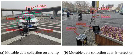
Figure 1.
Data collection method.
The raw LiDAR data generates points for all the scanned objects including ground points and noises, as shown in Figure 2.
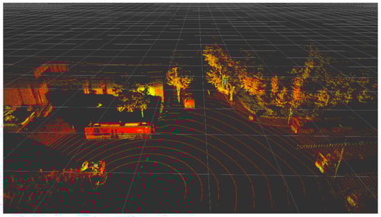
Figure 2.
Point cloud of LiDAR.
This paper used a data processing procedure introduced by Wu to process the roadside LiDAR data [31]. The data processing algorithms developed by Wu were further improved by other researchers [32,33,34,35]. This part briefly introduced the major parts of the data processing procedure. For the detailed information, we refer the readers to the reference [31]. The whole procedure contains three major steps: Background filtering, object clustering, and data association.
The purpose of background filtering is to exclude the irrelevant points and to keep the points of interest (moving objects) in the space. This paper used a density-based method named 3D-DSF for background filtering. The 3D-DSF firstly aggregates points in different frames into the same coordinate based on the points’ XYZ location. After aggregation, the space can be rasterized into same cubes with the same side length. Since the background points are relatively fixed, the cubes containing background points should have a higher point density compared to those cubes without background points. By giving a pre-defined threshold, the background cubes and non-background cubes can be distinguished. The locations of the background cubes are then stored in a matrix. The LiDAR data are searched by the matrix frame by frame, and any point found in the matrix is excluded from the space.
Points clustering is used to cluster the points belonging to one object into one group. The density-based spatial clustering of applications with noise (DBSCAN) was applied for object clustering by searching the distribution of point density in the 3D space [26]. Adaptive values were given to the two major parameters in the algorithm: Epsilon–the distance between two points to be covered in the same cluster, and minPts–the number of neighbors of one point to be included into a cluster.
To continuously track the same object, it is then necessary to associate the same cluster in different frames. The Global Nearest Neighbor (GNN) was employed for object tracking. This tracking algorithm utilizes the geometric location information of the vehicle to identify key points (nearest point to the LiDAR) in different frames belonging to the same object [36]. For each object in the current frame, the algorithm searches for the object with the minimum distance to the object in the previous frame.
The trajectories of road users can be generated after applying the data extraction procedure. Figure 3 shows an example of road users’ trajectories. The elements stored in each trajectory can be customized based on the requirement of different purposes. A summary of the typical elements in the trajectory can be found in Table 2. The accuracy of the trajectory has been well validated by checking the tracking speeds of the vehicles and the traffic volume in a previous study [31]. The results showed that about 98% of calculated speed had errors less than 2 mph by comparing the tracking speed and the speed extracted from the on-board diagnostic system information (OBD). For the detailed evaluation, we refer the readers to [31].
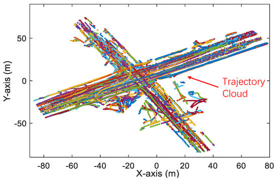
Figure 3.
Trajectories of road users.
Table 2.
Typical elements in the trajectory generated from roadside LiDAR.
The data were collected at six different sites in Jinan: G104 national road, East Erhuan road, Xinlongshan campus of Shandong University, on-ramp of around-city highway, Shungeng road, and Heping/Lishan intersection. Table 3 summarizes the sites.
Table 3.
Six sites for data collection.
Figure 4 shows the pictures of data collection at six sites.
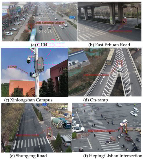
Figure 4.
Data collection sites.
3.2. Feature Selection
For simplicity, this paper defined four classes for the objects: Pedestrian, bicycle, passenger car (including pick-up), and truck (including bus). This paper did not consider motorcycle as one class since it was rarely captured on the urban roads. The researchers or traffic engineering can also define their own classes based on their purposes. For each road user, the corresponding point cloud can be created by the LiDAR and can be stored in the trajectory. The selected feature should reflect the difference between different classes. However, high quality and detailed features are either very sparse or very difficult to obtain. Therefore, the feature selection should consider whether the feature is extractable from the trajectories. Table 4 summarizes the features used in previous studies for LiDAR data classification.
Table 4.
Feature selection in previous studies.
All those previous studies used the shape/intensity information for object classification. Inspired by those previous studies in Table 4, this research selected five features for object classification considering the ease of calculation and characteristic representation. The five features are illustrated as follows.
- Number of points (NP). NP represents the number of LiDAR points in one object. NP can be easily obtained in the trajectory (from the point cloud package in Table 2).
- Max intensity change (MIC). MIC represents the difference between the max intensity of one point and the min intensity of one point in the point cloud package representing one object. MIC can be calculated bywhere i and j are LiDAR points in the point cloud package (P). i and j can represent the same point (i = j). Max Ini and Min Ini mean the max intensity of point i and the min intensity of point i, respectively.
- Distance between tracking point and LiDAR (D). D represents the nearest distance between the point cloud package and the roadside LiDAR. D can be calculated aswhere Tx, Ty, and Tz are the XYZ values of coordinate of the tracking point. It is assumed that the LiDAR reports its location as (0, 0, 0).
- Max distance in the XY plane (MDXY). MDXY represents the max distance between two points in the point cloud package in the XY plane. MDXX can be denoted aswhere m and n are any two points in the point cloud package (P) and m ≠ n. MDXX does not consider the value in the Z-axis.
- Max distance in Z-axis (MDZ). MDZ represents the max distance between two points in the point cloud package in the Z-axis. MDZ can be expressed aswhere i and j are any two points in the point cloud package (P). i and j can represent the same point (i = j). Zi is the Z-axis value of point i.
All five features can be directly calculated from the elements in the trajectory extracted from the LiDAR data.
4. Probabilistic Neural Network (PNN)
The probabilistic neural network (PNN) is one of the efficient neural networks that has been frequently applied for object classification [37]. PNN is usually faster and more accurate than the multilayer perceptron network, and is relatively insensitive to outliers [38]. PNN uses the Parzen estimators to approximate the probability distribution function (PDF) of each class. The multivariate Bayesian rule is implemented to allocate the class with the highest posterior probability to new input data. The structure of the PNN can be described as follows.
Assuming and are the PDFs associated with a p-dimensional input vector X for and , the misclassification cost ratio and the prior probability ratio can be expressed as
where ) is the cost of misclassification (one object was classified to but in fact it belonged to . is the prior probability of occurrence of population . The PDFs are used to estimate the posterior probability that belongs to class . The PDF in PNN is solved by the Bayesian classifier using Parzen estimator. In the case of the Gaussian kernel, the multivariate estimates [39] can be denoted as
where i is the pattern number, m is the total number of training patterns, is ith training pattern from category , б is the smoothing parameter, and p is the dimensionality of input space. can approximate any smooth density function.
A typical PNN can be illustrated in Figure 5. There are four layers in PNN: Input layer, pattern layer, summation layer, and output layer [37].
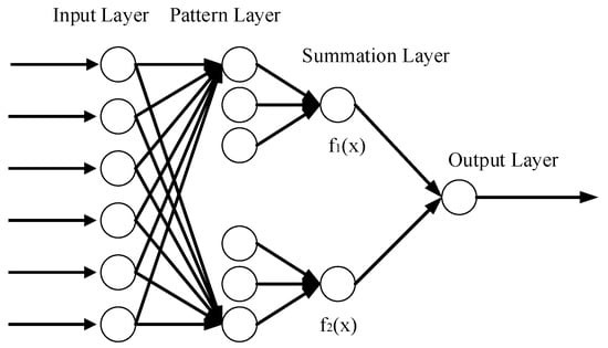
Figure 5.
PNN.
The input units are distribution units that supply the same input values to all the pattern units. Each pattern unit forms a dot product of the pattern vector X with a weight vector (). A nonlinear operation () was performed on Z before transferring the activation level to the summation layer. If we assume and are normalized to a unit length, the nonlinear operation can be expressed as
The nonlinear operation then is the same form as a Parzen estimator using a Gaussian kernel [40]. The summation unit sums the outputs for the pattern units corresponding to the category and calculates the PDFs. The output layer used the largest vote to predict the target category. Since the input pattern is used for the connection weights, PNN does not need adjusting for the connection weights. Therefore, the speed of training is much faster than the traditional back-propagation neural network (BP-NN).
5. PNN Training and Evaluation
5.1. Results of PNN
For the training database, a total of 2062 records were collected at six sites in urban Jinan, China. The selected three sites covered different scenarios (different Annual Average Daily Traffic (AADT), different pedestrian volumes, different light conditions, and different road types (intersection and road segment)). Among the 2062 records, 1446 of them were used for training and the other 616 records were used for validation. Another 674 records were collected at other two sites in Jinan, China for testing. For each site, a 360-degree camera is installed with the roadside LiDAR to capture the traffic situation. The roadside LiDAR is connected to GPS so that the LiDAR time can be synchronized with the camera time. Each record in the training and testing database was manually marked into one of the four classes by checking the corresponding video and the LiDAR data in the open-source software-RS-Viewer.
In this paper, PNN was implemented using the package “PNN” written in the statistical language-R [41,42]. The smoothing parameter was identified by the package automatically using a genetic algorithm [43]. To quantitatively evaluate the results of PNN, we applied the class-based accuracy (CA) to check the classification results. CA represents the percentage of total objects that are classified to the correct class. CA can be expressed as
where NR is the number of the actual records in class A. In this paper, A may be a bicycle, pedestrian, passenger car, or truck. NI is the number of records identified as class A by the algorithm. Table 5 shows the evaluation of the PNN model.
Table 5.
Evaluation of the PNN model.
It is shown that the accuracy of PNN classification using both a validation set and testing set was relatively high (more than 90%). As for the class-based results, the proposed method can even achieve a 100% accuracy for bicycle classification. The truck classification was the lowest. By checking the video, it was found that those trucks were misidentified as passenger cars (truck → passenger car) due to the package loss issue. Figure 6a,b show the package loss issue. There was a truck in Figure 6a, and all the points belonging to the truck were successfully clustered into one group. However, in Figure 6b, some packages were lost in the LiDAR data. As a result, a lot of sector-like areas without any LiDAR points showed up. The truck was cut by one sector-like area and was misclassified as two passenger cars. As for the pedestrian classification, the common error was that the pedestrians were misidentified as passenger cars (pedestrian → passenger car). This was caused by the pedestrians walking to close to each other. Figure 6c shows one pedestrian was crossing the road, and Figure 6d shows a group of pedestrians were crossing the road. Four pedestrians were walking close to each other in Figure 6d and the clustering algorithm mis-clustered the pedestrians into one group. Since the shapes of one pedestrian and the pedestrian group were significantly different, in the classification stage, the PNN then misclassified the pedestrian group as a passenger car. As for the classification of passenger car, the common error was that the passenger cars were misclassified as pedestrians (passenger car → pedestrian). This was usually caused by the occlusion issue--one vehicle was partially blocked by another one. With occlusion, only part of the vehicle was visible. Figure 6e shows that there were two passenger cars (marked as green and blue) and they were not blocked by each other. The PNN can successfully classify these two objects as two passenger cars. Figure 6f shows there were also two passenger cars (marked as green and blue) on the road and the most part of the blue car was blocked by the green car. As a result, the blue car was more like a pedestrian. The PNN then misclassified the blue car as a pedestrian. In fact, a lot of errors were not generated through the classification stage but the clustering stage. Therefore, the accuracy of the clustering can greatly influence the performance of the PNN algorithm.
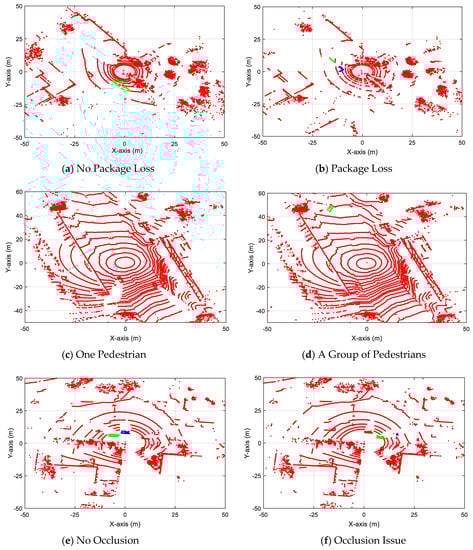
Figure 6.
Common errors in the PNN classification (2D View).
5.2. Results of PNN
A lot of other methods, including but not limited to BP-NN, naïve Bayes (NB), k nearest neighbor (KNN), support vector machine (SVM), and decision trees also have been widely used for object classification. In a previous study, it has shown that RF can provide better performance compared to NB, KNN [44]. Additionally, PNN has definite better performance compared to BP-NN [45]. Therefore, in this paper, NB, KNN, and BP-NN were not compared with PNN. The performance of SVM, random forest (RF), and PNN were compared in this section.
SVM is a nonlinear generalization of the generalized portrait algorithm. The goal of SVM is to establish a hyperplane that can maximize the distance between different classes and the hyperplane. Given a set with N training samples of points, the hyperplane meets
where N is the number of samples, is the label of the ith sample. and are two coefficients to be estimated by the SVM. In this paper, we used the radial basis function (RBF) as the kernel function for optimization in SVM.
RF classifier is a combination of tree classifiers that are generated using a random vector. RF can improve the accuracy of classification compared to a single decision tree by correcting the overfitting issue in the training set.
The same training database used for training PNN classifier was used to train the SVM classifier and RF classifier. Figure 7 illustrates the class-based accuracy of the three investigated methods.
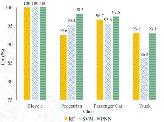
Figure 7.
CA of PNN, SVM, and random forest (RF).
It is clearly shown that PNN had a better performance than SVM and RF. The PNN can achieve an equivalent or higher accuracy compared to SVM and RF. Table 6 summarizes the confusion matrix of SVM, RF, and PNN by classifying the same testing database.
Table 6.
Confusion matrix.
It is shown that the misclassification type in the PNN usually happened in two classes (such as pedestrian → passenger car). The types of the misclassification in the SVM and the RF (such as pedestrian → bicycle/passenger car) were more discrete than that in the PNN. The overall accuracy of the PNN was also higher compared to the SVM and the RF.
6. Conclusions
This paper developed an object classification method for roadside LiDAR using PNN. An automatic data processing method to extract vehicle trajectories was introduced. A total of 2736 records were collected at six sites representing different scenarios. Five features were selected for PNN training. The input features can be automatically calculated using the data processing procedure. The overall accuracy of the PNN was 97.6%. The errors in the classification results were also diagnosed. Considering the accuracy and computational load, the performance of PNN was superior compared to other widely used classification methods (the RF and the SVM).
The misclassification errors generated by the PNN were diagnosed using the corresponding 360-degree camera. The object occlusion issue and/or package loss issue were the major reasons leading to the errors. In the real world, it is common that objects may be partially occluded by other objects. Modeling all those occlusion situations explicitly is computationally infeasible because of the variability of different situations. An easy and effective method is to install another LiDAR at a different location to overcome the object occlusion issue. The authors have conducted an early study for point registration for multiple LiDARs [46,47]. The performance of point registration for multiple LiDARs to reduce the occlusion issue needs to be further investigated. As for the package loss, there is still no effective solution to fix this issue. The connection between the LiDAR and the computer used for data processing should be carefully checked before starting the data collection to avoid the package loss issue. The current LiDAR data processing algorithm may mis-cluster two pedestrians close to each other as one pedestrian. The authors will try to find a solution to improve the accuracy of object clustering in the next step. The PNN cannot handle the data imbalance problem, which limits the accuracy of object classification. How to handle the data imbalance issue is another topic for future studies.
The future transportation system must rely on multiple sensors including LiDAR, camera, radar et al. The combination of data from different types of sensors can overcome the limitations of one single sensor and provide more complex features for classification. For example, thermal imaging, which has been widely used for fault diagnosis of electric impact drills, may be also used for object classification based considering that different road users may have different temperatures [48]. Therefore, it is also necessary to use the data from different sensors to further improve the accuracy of object classification [49]. How to integrate the data from different types of sensors is another research topic for future studies.
Author Contributions
Conceptualization, J.Z. and J.W.; methodology, J.Z., R.P. and J.W.; validation, X.M., Z.Y. and H.L.; investigation, J.Z.; writing—original draft preparation, J.Z.; writing—review and editing, J.W. All authors have read and agreed to the published version of the manuscript.
Funding
This research was funded part by the National Natural Science Foundation of China, grant number 52002224, part by the Natural Science Foundation of Jiangsu Province, grant number BK20200226, part by the Program of Science and Technology of Suzhou, grant number SYG202033, part by the Technical Program of Shandong Department of Transportation, grant number 2020BZ01-03, part by the Key Research and Development Program of Shandong Province, grant number 2020CXGC010118.
Data Availability Statement
The database is not open to the public for free now. But it may be obtained by contacting the corresponding author only for academic purposes.
Acknowledgments
The authors would like to thank all the editors and anonymous reviewers for their careful reading and insightful remarks.
Conflicts of Interest
The authors declare no conflict of interest.
References
- Wu, J.; Xu, H.; Zheng, Y.; Zhang, Y.; Lv, B.; Tian, Z. Automatic vehicle classification using roadside LiDAR data. Transp. Res. Rec. 2019, 2673, 153–164. [Google Scholar] [CrossRef]
- Wu, J.; Xu, H.; Zheng, Y.; Tian, Z. A novel method of vehicle-pedestrian near-crash identification with roadside LiDAR data. Accid. Anal. Prev. 2018, 121, 238–249. [Google Scholar] [CrossRef] [PubMed]
- Khan, M.A.; Kim, J. Toward Developing Efficient Conv-AE-Based Intrusion Detection System Using Heterogeneous Dataset. Electronics 2020, 9, 1771. [Google Scholar] [CrossRef]
- Zhao, J.; Xu, H.; Liu, H.; Wu, J.; Zheng, Y.; Wu, D. Detection and tracking of pedestrians and vehicles using roadside LiDAR sensors. Transp. Res. Part C Emerg. Technol. 2019, 100, 68–87. [Google Scholar] [CrossRef]
- Missoum, S. Controlling structure failure modes during an impact in the presence of uncertainties. Struct. Multidiscipl. Optim. 2007, 34, 463–472. [Google Scholar] [CrossRef]
- Wu, J.; Xu, H.; Sun, Y.; Zheng, J.; Yue, R. Automatic background filtering method for roadside LiDAR data. Transp. Res. Rec. 2018, 2672, 14–22. [Google Scholar] [CrossRef]
- Biljecki, F.; Ledoux, H.; Van Oosterom, P. Transportation mode-based segmentation and classification of movement trajectories. Int. J. Geogr. Inf. Sci. 2013, 27, 385–407. [Google Scholar] [CrossRef]
- Fuerstenberg, K.; Willhoeft, V. Object tracking and classification using laserscanners-pedestrian recognition in urban environment. In Proceeding of IEEE Intelligent Transportation Systems Conference, The Hague, The Netherlands, 6–9 October 2013; pp. 451–453. [Google Scholar]
- Gupte, S.; Masoud, O.; Papanikolopoulos, P. Vision-based vehicle classification. In Proceedings of the IEEE Intelligent Transportation Systems, Dearborn, MI, USA, 1–3 October 2000; pp. 46–51. [Google Scholar]
- Malinovskiy, Y.; Wu, Y.; Wang, Y. Video-based vehicle detection and tracking using spatiotemporal maps. Transp. Res. Rec. 2009, 2121, 81–89. [Google Scholar] [CrossRef]
- Zhang, G.; Avery, R.; Wang, Y. Video-based vehicle detection and classification system for real-time traffic data collection using uncalibrated video cameras. Transp. Res. Rec. 2007, 1993, 138–147. [Google Scholar] [CrossRef]
- Mithun, N.; Rashid, N.; Rahman, S. Detection and classification of vehicles from video using multiple time-spatial images. IEEE trans. Intell. Transp. Syst. 2012, 13, 1215–1225. [Google Scholar] [CrossRef]
- Chen, Z.; Ellis, T.; Velastin, S.A. Vehicle type categorization: A comparison of classification schemes. In Proceedings of the IEEE Intelligent Transportation Systems Conference, Washington, DC, USA, 5–7 October 2011; pp. 74–79. [Google Scholar]
- Zangenehpour, S.; Miranda-Moreno, L.; Saunier, N. Automated classification in traffic video at intersections with heavy pedestrian and bicycle traffic. In Proceedings of the TRB 93th Annual Meeting, Washington, DC, USA, 12–16 January 2014; pp. 492–509. [Google Scholar]
- Zangenehpour, S.; Miranda-Moreno, L.; Saunier, N. Automated classification based on video data at intersections with heavy pedestrian and bicycle traffic: Methodology and application. Transp. Res. Part C Emerg. Technol. 2015, 56, 161–176. [Google Scholar] [CrossRef]
- Liang, C.; Juang, C. Moving object classification using a combination of static appearance features and spatial and temporal entropy values of optical flows. IEEE trans. Intell. Transp. Syst. 2015, 16, 3453–3464. [Google Scholar] [CrossRef]
- Song, Y.; Zhang, H.; Liu, Y.; Liu, J.; Zhang, H.; Song, X. Background Filtering and Object Detection with a Stationary LiDAR Using a Layer-Based Method. IEEE Access 2020, 8, 184426–184436. [Google Scholar] [CrossRef]
- Lin, C.; Wang, K.; Wu, D.; Gong, B. Passenger Flow Prediction Based on Land Use around Metro Stations: A Case Study. Sustainability 2020, 12, 6844. [Google Scholar] [CrossRef]
- Lin, C.; Liu, H.; Wu, D.; Gong, B. Background Point Filtering of Low-Channel Infrastructure-Based LiDAR Data Using a Slice-Based Projection Filtering Algorithm. Sensors 2020, 20, 3054. [Google Scholar] [CrossRef] [PubMed]
- Cui, Y.; Xu, H.; Wu, J.; Sun, Y.; Zhao, J. Automatic vehicle tracking with roadside LiDAR data for the connected-vehicles system. IEEE Intell. Syst. 2019, 34, 44–51. [Google Scholar] [CrossRef]
- Khan, M.A.; Karim, M.; Kim, Y. Automatic vehicle tracking with roadside LiDAR data for the connected-vehicles system. Symmetry 2018, 10, 485. [Google Scholar] [CrossRef]
- Wu, J.; Xu, H.; Zhang, Y.; Tian, Y.; Song, X. Real-time queue length detection with roadside LiDAR data. Sensors 2020, 8, 2342. [Google Scholar] [CrossRef]
- Song, W.; Zhang, L.; Tian, Y.; Fong, S.; Liu, J.; Gozho, A. CNN-based 3D object classification using Hough space of LiDAR point clouds. Hum-cent. Comput. Inf. 2020, 10, 1–14. [Google Scholar] [CrossRef]
- Premebida, C.; Monteiro, G.; Nunes, U.; Peixoto, P. A lidar and vision-based approach for pedestrian and vehicle detection and tracking. In Proceedings of the IEEE Intelligent Transportation Systems Conference, Seattle, WA, USA, 30 September–3 October 2007; pp. 1044–1049. [Google Scholar]
- Lee, H.; Coifman, B. Side-fire lidar-based vehicle classification. Transp. Res. Rec. 2012, 2308, 173–183. [Google Scholar] [CrossRef]
- Zhang, F.; Clarke, D.; Knoll, A. Vehicle detection based on LiDAR and camera fusion. In Proceedings of the IEEE Intelligent Transportation Systems Conference, Qingdao, Shandong, China, 8–11 October 2014; pp. 1620–1625. [Google Scholar]
- Yao, W.; Hinz, S.; Stilla, U. Extraction and motion estimation of vehicles in single-pass airborne LiDAR data towards urban traffic analysis. ISPRS J. Photogramm. 2011, 66, 260–271. [Google Scholar] [CrossRef]
- Song, Y.; Tian, J.; Li, T.; Sun, R.; Zhang, H.; Wu, J.; Song, X. Road-Users Classification Utilizing Roadside Light Detection and Ranging Data. SAE Tech. Pap. 2020. 2020-01-5150. [Google Scholar] [CrossRef]
- Gao, H.; Cheng, B.; Wang, J.; Li, K.; Zhao, J.; Li, D. Object classification using CNN-based fusion of vision and LIDAR in autonomous vehicle environment. IEEE Trans. Ind. Electron. 2018, 14, 4224–4231. [Google Scholar] [CrossRef]
- Wang, H.; Wang, B.; Liu, B.; Meng, X.; Yang, G. Pedestrian recognition and tracking using 3D LiDAR for autonomous vehicle. Rob. Auton. Syst. 2017, 88, 71–78. [Google Scholar] [CrossRef]
- Wu, J. An automatic procedure for vehicle tracking with a roadside LiDAR sensor. Ite J. 2018, 88, 32–37. [Google Scholar]
- Liu, H.; Lin, C.; Wu, D.; Gong, B. Slice-Based Instance and Semantic Segmentation for Low-Channel Roadside LiDAR Data. Remote Sens. 2020, 12, 3830. [Google Scholar] [CrossRef]
- Song, X.; Wu, J.; Zhang, H.; Pi, R. Analysis of Crash Severity for Hazard Material Transportation Using Highway Safety Information System Data. SAGE Open 2020, 10, 2158244020939924. [Google Scholar] [CrossRef]
- Wu, J.; Song, X. Review on smart highways critical technology. Int. J. Eng. Sci. 2020, 50, 52–69. [Google Scholar]
- Wang, G.; Wu, J.; Xu, T.; Tian, B. 3D Vehicle Detection with RSU LiDAR for Autonomous Mine. IEEE Trans. Veh. Technol. 2021, 70, 344–355. [Google Scholar] [CrossRef]
- Wu, J.; Xu, H.; Tian, Y.; Pi, R.; Yue, R. Vehicle detection under adverse weather from roadside LIDAR Data. Sensor 2020, 20, 3433. [Google Scholar] [CrossRef]
- Gargoum, S.; El-Basyouny, K.; Sabbagh, J.; Froese, K. Automated highway sign extraction using lidar data. Transp. Res. Rec. 2017, 2643, 1–8. [Google Scholar] [CrossRef]
- Specht, D.F. Probabilistic neural networks. Neural Netw. 1990, 3, 109–118. [Google Scholar] [CrossRef]
- Specht, D.F. A general regression neural network. IEEE Trans. Neural Netw. 1991, 2, 568–576. [Google Scholar] [CrossRef] [PubMed]
- Abdulhai, B.; Ritchie, S.G. Enhancing the universality and transferability of freeway incident detection using a Bayesian-based neural network. Transp. Res. Part C Emerg. Technol. 1999, 7, 261–280. [Google Scholar] [CrossRef]
- Cacoullos, T. Estimation of a multivariate density. Ann. Inst. Stat. Math. 1966, 18, 179–189. [Google Scholar] [CrossRef]
- Oh, C.; Kang, Y.S.; Youn, Y.; Konosu, A. Development of probabilistic pedestrian fatality model for characterizing pedestrian-vehicle collisions. Int. J. Automot. Technol. 2008, 9, 191–196. [Google Scholar] [CrossRef]
- Chasset, P.O. Probabilistic Neural Network for the R Statistical Language. 2013. Available online: http://flow.chasset.net/pnn (accessed on 14 March 2021).
- Yue, R.; Xu, H.; Wu, J.; Sun, R.; Yuan, C. Data registration with ground points for roadside LiDAR sensor. Remote Sens. 2019, 11, 1354. [Google Scholar] [CrossRef]
- Wu, J.; Zhang, Y.; Tian, Y.; Yue, R.; Zhang, H. Automatic Vehicle Tracking with LiDAR-Enhanced Roadside Infrastructure. J. Test Eval. 2021, 49, 121–133. [Google Scholar] [CrossRef]
- Wu, J.; Xu, H.; Tian, Y.; Zhang, Y.; Zhao, J.; Lv, B. An automatic lane identification method for the roadside light detection and ranging sensor. J. Intell. Transp. Syst. 2020, 24, 467–479. [Google Scholar] [CrossRef]
- Lv, B.; Xu, H.; Wu, J.; Tian, Y.; Tian, S.; Feng, S. Revolution and rotation-based method for the roadside LiDAR data integration. Opt. Laser Technol. 2019, 119, 105571. [Google Scholar] [CrossRef]
- Glowacz, A. Fault diagnosis of electric impact drills using thermal imaging. Measurement 2021, 171, 108815. [Google Scholar] [CrossRef]
- Wu, J.; Xu, H.; Liu, W. Points Registration for Roadside LiDAR Sensors. Transp. Res. Rec. 2019, 2673, 627–639. [Google Scholar] [CrossRef]
Publisher’s Note: MDPI stays neutral with regard to jurisdictional claims in published maps and institutional affiliations. |
© 2021 by the authors. Licensee MDPI, Basel, Switzerland. This article is an open access article distributed under the terms and conditions of the Creative Commons Attribution (CC BY) license (http://creativecommons.org/licenses/by/4.0/).