Article

Complex-Valued Pix2pix—Deep Neural Network for Nonlinear Electromagnetic Inverse Scattering

College of Control Science and Engineering, China University of Petroleum, Qingdao 266000, China
*
Author to whom correspondence should be addressed.
Electronics 2021, 10(6), 752; https://doi.org/10.3390/electronics10060752
Submission received: 2 March 2021 / Revised: 18 March 2021 / Accepted: 19 March 2021 / Published: 22 March 2021
(This article belongs to the Section Microwave and Wireless Communications)

Abstract

:
Nonlinear electromagnetic inverse scattering is an imaging technique with quantitative reconstruction and high resolution. Compared with conventional tomography, it takes into account the more realistic interaction between the internal structure of the scene and the electromagnetic waves. However, there are still open issues and challenges due to its inherent strong non-linearity, ill-posedness and computational cost. To overcome these shortcomings, we apply an image translation network, named as Complex-Valued Pix2pix, on the inverse scattering problem of electromagnetic field. Complex-Valued Pix2pix includes two parts of Generator and Discriminator. The Generator employs a multi-layer complex valued convolutional neural network, while the Discriminator computes the maximum likelihoods between the original value and the reconstructed value from the aspects of the two parts of the complex: real part and imaginary part, respectively. The results show that the Complex-Valued Pix2pix can learn the mapping from the initial contrast to the real contrast in microwave imaging models. Moreover, due to the introduction of discriminator, Complex-Valued Pix2pix can capture more features of nonlinearity than traditional Convolutional Neural Network (CNN) by confrontation training. Therefore, without considering the time cost of training, Complex-Valued Pix2pix may be a more effective way to solve inverse scattering problems than other deep learning methods. The main improvement of this work lies in the realization of a Generative Adversarial Network (GAN) in the electromagnetic inverse scattering problem, adding a discriminator to the traditional Convolutional Neural Network (CNN) method to optimize network training. It has the prospect of outperforming conventional methods in terms of both the image quality and computational efficiency.

1. Introduction

As an accurate and non-destructive measurement modality for imaging, nonlinear electromagnetic inverse scattering is widely used in science, engineering, military and medical fields [1,2,3,4,5]. Compared with conventional tomography methods [6,7,8,9,10], nonlinear electromagnetic inverse scattering can solve the multiple scattering problem of electromagnetic wave fields inside the object [3,4,5,11], and the internal structure of the scene can be “seen“ in a quantitative way. A large number of algorithms have been proposed and developed over the past few decades to solve electromagnetic inverse scattering problem, which can be divided into the following two: (a) deterministic optimization methods including Distorted Born iterative methods (DBIM) [12,13], Subspace based Optimization (SOM) [14,15,16,17,18], Contrast Source Inversion [19,20,21], and (b) stochastic methods [22,23,24] such as Particle Swarm Optimization Algorithms (PSO). In recent years, with the widely studied and rapidly developed of compressive sensing theory, some inverse scattering methods were produced for addressing the problem of Synthetic Aperture Radar(SAR) imaging [25,26,27,28]. Despite it has been verified that these methods can provide satisfactory results for objects of intermediate size and contrast. Owing to the limitation of computational costs, it is still a great challenge to apply them to large and realistic scenes. So far, with the effect of multi-scattering effects, the nonlinear electromagnetic inverse scattering technique is primarily used with low-contrast objects. And it is hard to handle the high-frequency scene.
Over the past years, deep neural network has been widely used in regression and classification problems [29,30]. With the establishment of massive databases and the improvement of computing power, depth neural network (DNN) has become one of the most powerful methods in the fields of image processing and computer vision, such as semantic segmentation [31], Depth Estimation [32], Image Deblurring [33] or Super Resolution Reconstruction [34,35]. Deep learning methods have been proven to be helpful in the design and implementation of advanced functional materials [36] and high-precision reconstruction from compression measurements [37,38]. The DNN method has also been proved to be superior to the traditional machine learning method in automatic analysis of the high content microscope data [39]. Recently, DNN algorithm has been widely used in the field of imaging, such as biomedical imaging, including Magnetic Resonance imaging (MR) and SAR imaging [40] and X-ray Computed Tomography [41,42] and Computational Optical Imaging [11,43,44], as well as the DeepNIS method [45]. The experimental results show that, compared with the conventional image reconstruction methods, the algorithm based on neural networks [46,47] and the strategy based on DNN can greatly reduce imaging time and improve the imaging quality significantly [41,42,43,44,45,46,47,48]. However, traditional DNN requires a large amount of training samples to generate a trained network, which needs more time in terms of training.
We propose an image translation network, named Complex-Valued Pix2pix (CVP2P). Our solution strategy is first inspired by the Back-Propagation Scheme (BPS) [49] and then the conventional CNN is replaced by the CVP2P network. The CVP2P is a straightforward extension of the traditional pix2pix [50], a deformation of conditional generative adversarial network, which inheriting the advantages of the latter. CVP2P mainly consists of two parts—generator and discriminator. The generator is similar to a traditional CNN method and can generate the final solution. The role of the discriminator is to make the generator capture more nonlinear features than traditional CNN by the confrontation training between the two. When the object has high contrast with high working frequency, the inverse scattering problem is highly nonlinear. Thus, the CNN for BPS can hardly capture all nonlinear features. In comparison, the CVP2P can learn the mapping from input to output more quickly by confrontation training between generator and discriminator. This can effectively reduce the network training time than traditional CNN methods. The proposed scheme can be divided into two stages:
  • (Stage I) An initial guess of the contrast
  • (Stage IIc) Obtain a better contrast estimation through a custom deep learning network.
In this paper, an initial guess of the contrast is obtained by back-propagation method. We will demonstrate that the CVP2P network can efficiently reconstruct the targets with higher accuracy and efficiency than others. The input data of CVP2P originates from the back-propagation results in Stage (I) and the input label comes from the real contrast of the corresponding model.
The content of this paper is as follows—Section 2 states the problem and explains the final estimated goal of the electromagnetic inverse scattering problem. Section 3 describes the two stages of the above methods and compares the related schemes. Section 4 describes the implementation details of the network, including loss function, network structure and the training of the network. In Section 5, simulation and experiments are conducted to verify the performance of CVP2P. We used the MNIST dataset to train and test the CVP2P network [51]. We also built a microwave imaging system to provide experimental data for the algorithm to test the generalization ability of the algorithm. Finally, the whole paper is concluded and analyzed in the Section 6.

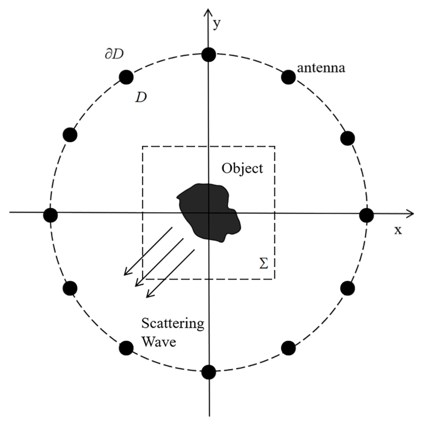
2. Problem Statement

A two-dimensional scalar electromagnetic field is considered in this paper. As shown in Figure 1, the incident plane wave E z , i n of TM polarization irradiates the target region Σ . And the subscript z represents the Z component of electromagnetic waves. N S receivers with distance R from origin are uniformly distributed on D and used to receive scattering field data. The scattered field received by the receiver can be expressed as:
E z , s c a ( r ) = k 0 2 Σ G ( r , r ) χ ( r ) E z ( r ) d S r D , r Σ ,
E z ( r ) = E z , i n ( r ) + k 0 2 Σ G ( r , r ) χ ( r ) E z ( r ) d S r Σ , r Σ ,
r and r Σ represent the field point and the source point, respectively. d S is an area unit on Σ . E z ( r ) represents the total field, χ ( r ) = ε r ( r ) 1 i ( σ ( r ) ε 0 ω ) denotes a quantitative relationship between the contrast of the object χ ( r ) and relative permittivity ε r ( r ) . σ ( r ) , ε 0 and ω are conductivity, vacuum permittivity and angular frequency, respectively. G ( r , r ) = i 4 H 0 ( 1 ) ( k 0 r r ) denotes the two-dimensional Green’s function, H 0 ( 1 ) ( ) denotes the first kind of zero order Hankel function.
The scattered field is measured with N S receivers per illumination with a total of N I illuminations in a single experiment. In order to carry out numerical experiments, we solve the discretized version of the Equations (1) and (2) by partitioning Σ into an K × K square grid using the method of moments. Meanwhile, the product of the contrast χ and the internal field E ( r ) at any point r in Σ is defined as the contrast source w , as shown in Equation (5). Combined with Equations (1) and (2), we obtain the following associated discretized forms:
e j n = e in j n + G S w j n
e sca j n = G M w j n
w j n = χ n e j n ,
where e j n C K 2 × 1 , e in j n C K 2 × 1 denotes the total internal and incident fields for the j-th illumination, respectively. And n is the number of iterations. w j n C K 2 × 1 denotes the contrast source, e sca j n C N S × 1 refers to the scattered field, e j n , e in j n and e sca j n represent the discretized version of E z ( r ) , E z , i n ( r ) and E z , s c a ( r ) , respectively. χ n C K 2 × 1 refers to the contrast in the imaging domain Σ . G S C K 2 × K 2 and G M C N S × K 2 represents the state matrix and measurement matrix, respectively.
The inverse scattering problem is to use the known scattered field e sca to estimate the contrast χ .

3. Methods

3.1. Motivation

The equations between the scattering field and the object contrast, such as Equations (3)–(5), are non-linear and ill-conditioned equations, therefore the system will have infinite solutions when solving the inverse problem. So it is difficult to choose a meaningful solution. This defect is especially obvious under the conditions of high contrast objects or high frequency scene.
Although it is possible to learn the mapping from the scatter field e sca to the contrast χ directly, we can also pre-process the scattered data e sca using non-iterative inversion algorithm before training the network. Accordingly, we propose a two stage strategy based on back-propagation method, which is a computationally simple and effective solution for highly non-linear inverse scattering problem. Next, we will explain the individual stages of this deep learning scheme.

3.2. Initial Guess (Stage-I)

Similar to the method adopted by CSI, we use the back-propagation (BP) algorithm to determine the initial value of the contrast source as follows
w j 0 = G M * e sca j Σ 2 G M G M * e sca j D 2 G M * e sca j ,
where w j 0 represents the initial value of the contrast source. G M * is the adjoint matrix of the measurement matrix G M , · Σ 2 represents the 2-norm in the target area Σ , · D 2 and represents the 2-norm on the measurement boundary D .
According to the state equation of Equation (2) and the initial value of the contrast source of Equation (6), the initial value of the total field e j 0 can be obtained as follows.
e j 0 = e in j + G S w j 0 .
Thus, the initial value of contrast χ 0 can be computed by the following Equation (8).
χ 0 = j w j 0 e j 0 * j e j 0 2 .
Combining the above Equation (6) to Equation (8), the initial contrast χ 0 can be prepared as the input of the subsequent CVP2P network.

3.3. Comparison with Related Schemes

A popular deep learning method for dealing with inverse problems is the DCS method [49]. In the learning process of DCS, the contrasts χ of each incidence are put into different input-channels of CNN, and each corresponding output-channel is the true contrast χ of the domain Σ . Consequently, there are N pairs of input- and output-channels in DCS, obviously different from BPS with only one pair of input- and output-channel. Thus for DCS, results from different incidences are filled into different channels of the input images, which is helpful to capture more nonlinear features. In CVP2P, the discriminator as a loss function has its nature advantage of capturing more inner nonlinear features because of the compromise between the generator and the discriminator. Thus it probably has similar advantages as DCS in terms of capturing more nonlinear features with deeper length and confrontation strategy other than more channels.
As a related inversion procedure based on deep learning, the contrast source network (CS-Net) has recently been proposed to solve the inverse scattering problem [48]. CS-Net trains the network to learn the noise subspace components of the contrast source, so as to obtain an estimation of the total contrast source. Its final output is still obtained by the iterative algorithm of CS, which fails to discard the long time procedure of iteration. While the CVP2P replaces the iterations with the deep learning network, which make the main difference between them.

4. Implementation Details of the Network

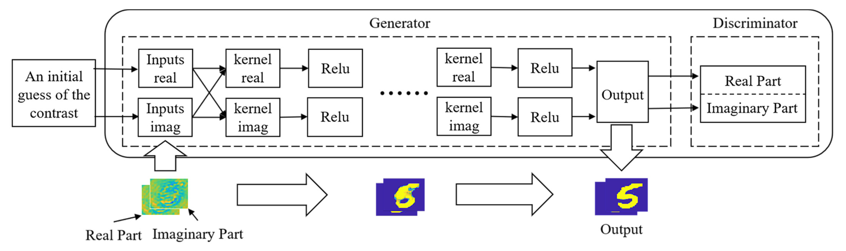
4.1. Structure and Core Idea of CVP2P

The CVP2P is a kind of Generative Adversarial Network (GAN) [52], which has similar structure to the network of pix2pix. Different from the traditional pix2pix to learn the mapping from input picture to output picture, CVP2P mainly learns the mapping from input complex data to output complex data.
CVP2P mainly consists of two parts—generator and discriminator. The role of the generator is to try to fool the discriminator by generating a contrast as accurate as possible, and the discriminator needs to distinguish as much as possible between the real contrast and the contrast generated by the generator. Through confrontation training, both continuously optimize their own network to achieve a balance point, so that the contrasts generated by the generator are infinitely close to the real samples. In the end, we can obtain an ideal generator to generate the desired result. Thus, it can be seen that the best advantage of CVP2P is that the updated information of generator (G) comes from discriminator (D) rather than the data sample. For example, if we give the generator the goal of “learning the mapping between input data and output data”, the discriminator will control the generator to achieve this goal by confrontation training between them.
The generator of traditional image translation network (pix2pix) adopts U-net structure and is composed of convolution and deconvolution neural network. The discriminator adopts “PatchGAN” architecture and is composed of convolution neural network. The traditional pix2pix network is difficult to be applied directly to the electromagnetic inverse scattering problem because it cannot deal with the complex. To solve this difficulty, we have made the following improvement. Firstly, the generator of CVP2P adopts a multilayer complex-valued Convolution Neural Network (cCNN), which can compute the complex-valued convolution and apply activation function on both real and imaginary parts respectively. Different filter size is used in different cCNN layer to capture the features from different spatial scales. And then the discriminator is divided into two parts: real part and imaginary part. Either discriminator is a small traditional CNN that adopts “Patch-GAN“ architecture. The complex generated by the generator is sent to the corresponding discriminator for judgment.

4.2. CVP2P Loss Function

The loss function of the CVP2P is inspired by the traditional pix2pix. It combines the loss function of cGAN with L1 distance, both of which should be calculated by the law of complex. Thus, the loss function of cGAN and L1 distance are expressed as the following Equations (11) and (12) respectively:
L c G A N ( G , D r / i ) = E x r / i , y r / i P d a t a ( x r / i , y r / i ) [ log D r / i ( x r / i , y r / i ) ] + E x r / i P d a t a ( x r / i ) [ l o g ( 1 D r / i ( x r / i , G ( x r / i ) ) ) ]
and
L c o m p l e x ( G ) = E y r p d a t a ( y r ) [ | | y r G ( y r ) | | 1 ] + E y i p d a t a ( y i ) ( z ) [ | | y i G ( y i ) | | 1 ] ,
where G tries to generate the estimation of contrast. D r / i represents the real r or imaginary i parts of discriminator, aims to distinguish between Ground Truths y r / i and G ( x r / i ) generated estimation of contrast. L c o m p l e x ( G ) is the complex value of L1 distance.
Thus, the final loss function of CVP2P becomes as follows, where λ controls the relative importance of the two loss function:
G * = arg min G max D [ L c G A N ( D r , G ) + L c G A N ( D i , G ) + λ L c o m p l e x ( G ) ] .

4.3. CVP2P: Network Training

The structural details of the CVP2P for nonlinear inverse scattering are described in Figure 2. The input data of the CVP2P comes from the BP algorithm.
The training procedure for the CVP2P is as follows:
(1)
In the first step, the initial contrasts are divided into the real part and the imaginary part as the input of the generator. And then both parts are convolved with the corresponding filters according to Equation (10) to obtain a set of feature matrices. Note that the output of cCNN has the same size as its input. In other words, the size of the feature matrix remains constant in entire training process.
(2)
In the second step, these feature matrices undergo a nonlinear activation function to obtain a sparse outcome. Then the result is used as the input of the next layer to repeat above operation. Generally speaking, it is assumed that the relative permittivity is not smaller than 1 and the conductivity is non-negative. Therefore, the real part of the contrast is positive and the imaginary part of the contrast is negative. If we use the activation function of ReLu, we should apply the ReLu function to the complex conjugate of the contrast.
(3)
In the third step, the output of the final cCNN is sent to the corresponding discriminator for discrimination.
The results of a different number of convolution layers in the generator are tested. The experimental results show that a 9-layers convolution is sufficient to achieve the desired image quality. If necessary, more convolution layers can be added to enrich the nonlinearity of the network. But, this enhances the complexity of the network, which requires additional training cost and enhances the likelihood of overfitting. Since the main role of the discriminator is to train the generator, two convolution layers are sufficient to obtain the ideal generator in the case we consider.

5. Numerical and Experimental Results

The performance of CVP2P is assessed from the two aspects of simulation and experiment. For comparison, we also test the corresponding results of the Multiplicative Regularization Contrast Source Inversion (MR-CSI) method, both of which employ the Green’s integral equation to generate the measured data in simulation as Equations (1) and (2).

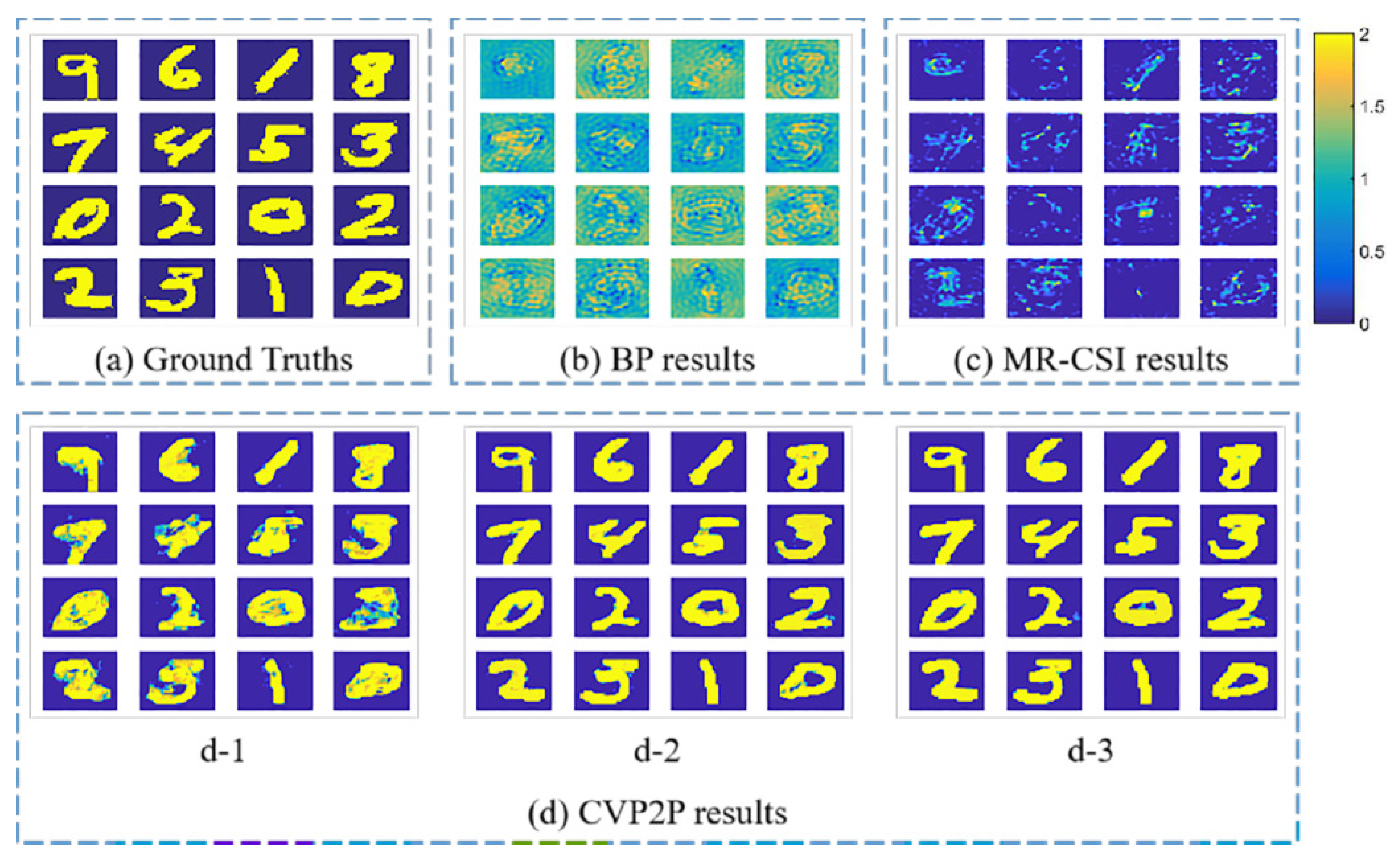
5.1. Training and Testing over MNIST Dataset

The MNIST handwritten digit dataset is used to evaluate CVP2P. As common handwritten digits dataset in the field of deep learning, the MNIST dataset is commonly adopted to train and test networks. When the CVP2P method is applied to non-destructive testing, the permittivity of foreign object generally has a simple distribution with the shape of circle, ellipse or striped shape. The relative permittivity value is relatively concentrated in a certain range. Thus, we use some simplified samples, such as the MNIST handwriting digit dataset, as the training set to obtain their characteristics for foreign object detection, because they have the similar shape or distribution characteristics. For simplification, We use binary handwritten digit sets for training to test constant contrast objects with different shapes. Referring to Figure 1, the imaging region Σ is a square with size of 5 . 6 λ 0 × 5 . 6 λ 0 ( λ 0 = 7 . 5 cm is the effective wavelength in vacuum). For numerical simulation, the imaging region Σ is composed of 110 × 110 uniform sub-squares. 32 transmitting antennas are uniformly distributed on the circular region D containing the imaging region Σ . And the radius of this region is represented by R = 10 λ 0 . Meanwhile, 32 receiving antennas are used to collect the scattered electric field of the probed scene. The relative permittivity ε r of digit-like objects are equal to 3, in this full-wave electromagnetic simulation [53]. In addition, in order to test the ability of the network, we consider adding 10% random white noise to data of the scattered field for testing in this research. Note that we only train CVP2P in the noiseless case and test the network with noise-added data. From the MNIST dataset, we randomly select 7000 images as the samples’ contrast. Through solving the full-wave solution of Maxwell’s equations, the electromagnetic responses of multiple inputs and multiple outputs are obtained. Afterwards, 7000 BP results can be generated as initial contrast. These data are used as the input of CVP2P, while the 7000 samples’ contrasts are considered to be the input label and expected output of CVP2P. As a result, 7000 data pairs are randomly broken into two groups: 6000 for network training, and 1000 for network testing.
The training of CVP2P was administered by the ADAM optimization method [54], and the epoch setting is 12. The learning rates are set to 0.0002. The filters are initialized randomly. All computations are performed in a small-scale server with the configuration of 128 GB access memory, with Intel Xeon E5-1620v2 central processing unit and NVIDIA GeForce GTX 1080Ti. We implemented and trained the CVP2P using Tensorflow library [55]. And the MR-CSI algorithms are implemented in Matlab 2018. Each iteration (including forward and backward pass) takes about 1.2s, and the complete training takes about 4h.
Figure 3a shows the ground truths of the simulated MNIST handwritten digits for the nonlinear inverse problem. Figure 3b,c show the image obtained by BP and the MR-CSI with 1000 iterations, respectively. This is a clear indication that neither BP nor MR-CSI can provide acceptable results in high contrast cases. The corresponding results that calculated by CVP2P with cCNNs of 3, 6, and 9 layers are shown in Figure 3d(d-1,d-2,d-3), respectively. The results illustrate that more parts of the nonlinear features in inverse scattering problem can be learned by CVP2P.
In order to compare the impact of different methods on imaging quality, the so-called Peak Signal to Noise Ratio (PSNR) and Correlation Coefficient (CC) are used as qualitative measure metrics to assess image quality. For CVP2P method, the results of cCNN with 9 layers are selected to evaluate the image quality, because it can be seen intuitively that the reconstruction result of cCNN with nine layers is better for all the cases we consider. The formula to calculate CC and PSNR are as follows:
C C = C o v ( X , Y ) D ( X ) D ( Y )
P S N R = 20 log ( M A X I M S E ) ,
where X is the real part of the reconstruction, Y is the real part of the original model, D ( · ) and C o v ( · ) represent the variance operator and covariance operator, respectively. The possible maximum pixel value is represented by M A X I . M S E is the Mean Square Error between the original image and the reconstructed image. Table 1 and Table 2 respectively show the corresponding peak signal-to-noise ratio (PSNR) and CC of different methods.
As can be seen from the above table, the value of the qualitative measure metrics for CVP2P is much higher than the traditional method. And for PSNR and CC, higher values mean better image quality.
We note that in this case, the well-trained CVP2P, BP and MR-CSI algorithm takes about 1 s, 8 s and 10 min to reconstruct an image, respectively. The computation time of the CVP2P is much faster than the traditional method. Accordingly, it can be concluded that the CVP2P is significantly better than MR-CSI method from two aspects of image quality and computation time in this high-contrast case. Moreover, we also consider the architecture with more cCNN layers to learn more multiple scattering rules for improving the imaging quality. In the inverse scattering problem, we usually hope that the reconstruction result is consistent with the ground truth. However, the PSNR value fails to keep in line with the subjective judgment of human eye. In other words, when the PSNR value is high, the reconstruction may be unsatisfactory. PSNR performs poorly in predicting subjective image quality. Thus, the CC becomes the only indicator to evaluate the imaging quality in later cases.

5.2. Testing over Letter Targets with Trained Networks

We carry out another set of numerical simulations so as to verify the superiority of the method. In this test, the MNIST dataset is still invoked as the training set of CVP2P. Meanwhile, the test objects have the shape of English letters and the relative permittivity is set to 3. Other parameters are all the same as the Example 1.
Figure 4 shows the reconstruction results based on different inverse scattering methods, where ground truths is displayed in the first row. The imaging results of the BP, MR-CSI and CVP2P are illustrated in the second, third and fourth rows, respectively. We use CC to compare the image quality of the reconstruction with all the three methods above, which is shown in the Table 3. Moreover, the reconstruction time with the trained CVP2P takes less than 1 s, while the MR-CSI method takes the reconstruction time of about 10 min with 1000 iterations. The BP algorithm takes 8 s because of its low computational complexity. Because the probed object has relative high contrast, the MR-CSI method unable to produce satisfactory reconstruction results. Therefore, the CVP2P exhibits significantly better than BP and MR-CSI from the aspects of imaging quality and time.
Through the above discussion, we can conclude that although the network is only trained by the MNIST dataset, we can still obtain satisfactory reconstruction results for different types of objects with the trained CVP2P. This indicates that the CVP2P can learn the generalizable mapping between ground truth and the input in a similar electromagnetic inverse scattering scenario regardless of the shapes of scatters. We clearly observed that the CC of the CVP2P method is much higher than the BP and MR-CSI method. In other words, the CVP2P can learn more accurate features of the nonlinear imaging models.

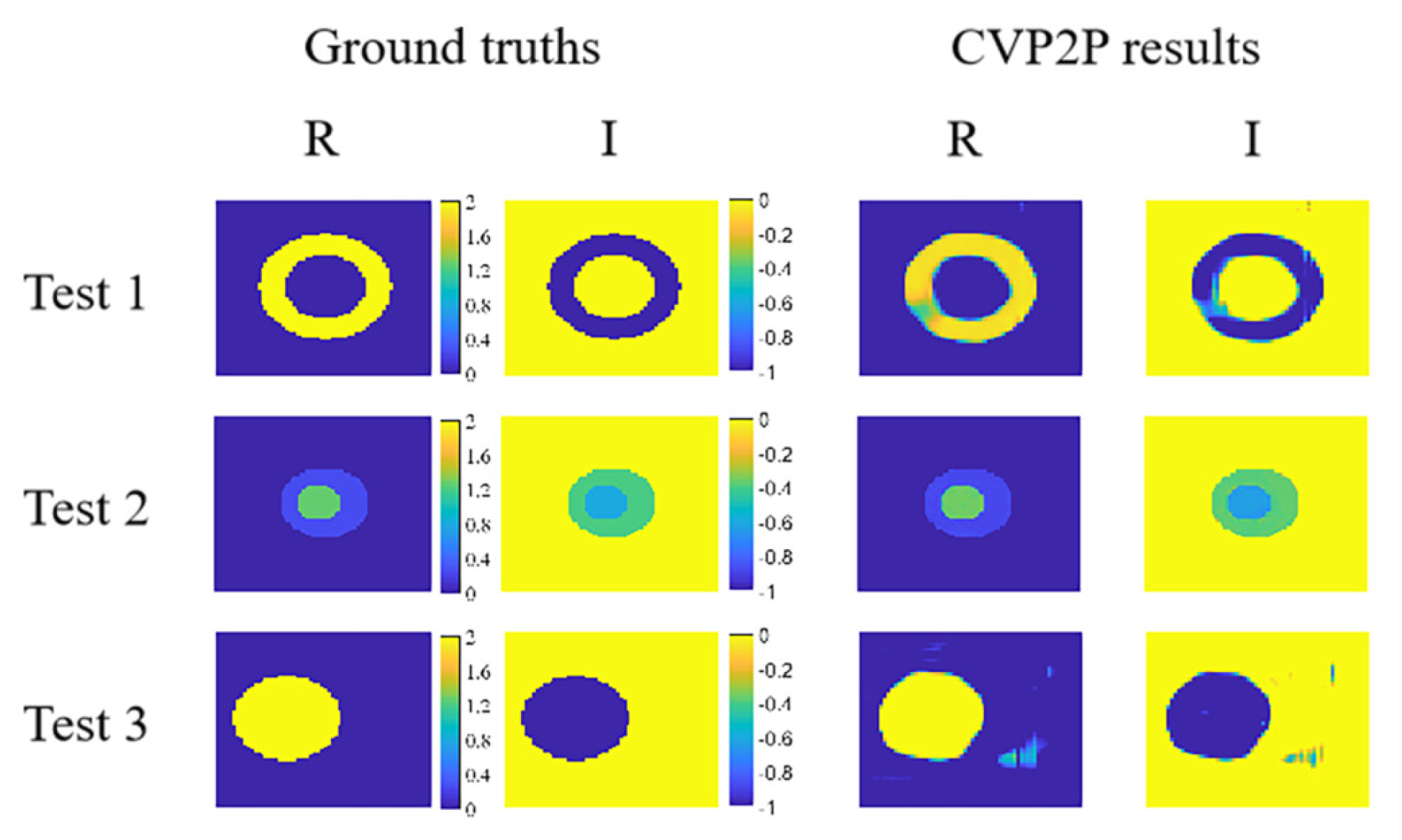
5.3. Tests with Lossy Scatterers

We further verify the versatility of the CVP2P method by reconstructing lossy scatterers. Other parameters are all the same as the Example 1 except for the complex value contrast.
In the first two columns of Figure 5, the true profiles of three ground truths are shown. The real and imaginary parts of relative permittivity are in the range of 1–3 and 0–1 in the training set of Example 3, respectively. The reconstructed results by the CVP2P are also displayed in Figure 5, and it is seen that these scheme achieve acceptable results for lossy scatterers. We use CC to compare the image quality of the reconstruction with real and imaginary parts, which is shown in the Table 4.

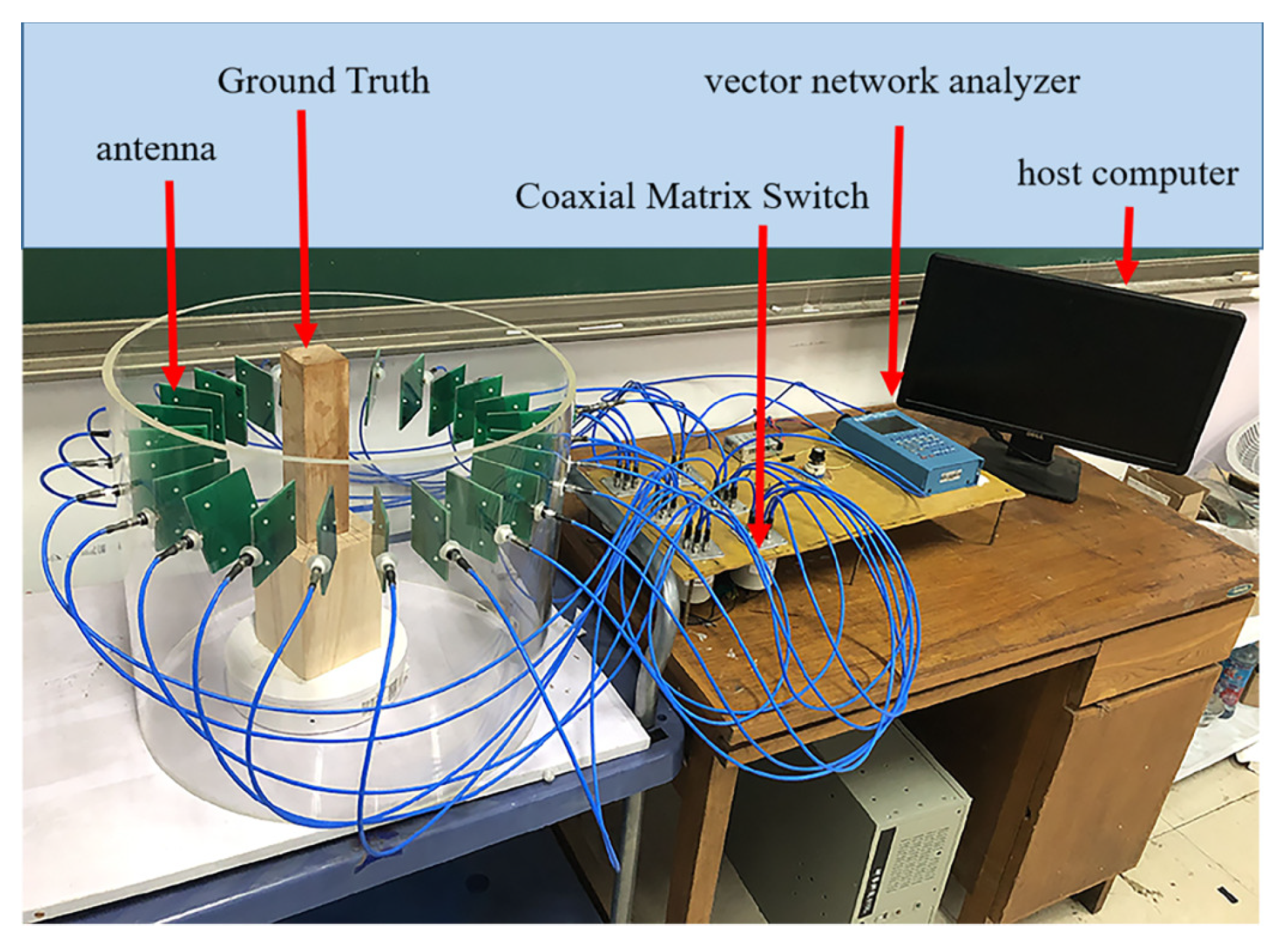
5.4. Testing Pre-Trained Networks by Experimental Data

In order to have a deeper understanding on CVP2P, the homemade measurement system for imaging are used to obtain Experimental data of antenna array for generalizability verification. We first built a Multi-antenna measurement system to provide experimental data. The picture of the experimental system is shown in Figure 6.
The system works at 3–5 GHz with 24 balanced Vivaldi antennas, which are evenly placed on a cylinder with a radius of 22.5 cm. Each Vivaldi antenna is 7 cm long, and it is 7.3 cm wide.The maximum imaging domain, D, consisted of a circle of radius 17 cm, located at the center of the chamber. If a square domain is used, the maximum size is a length of 18 cm. In practice, we have used a maximum imaging domain, D, with 10 cm sides. A vector network analyzer (KC901V) is connected to antenna via Agilent Coaxial Matrix Switch for transmitting and receiving signals, which provided port isolation of greater than 100 dB over the frequency range of interest. A host computer is connected to the vector network analyzer via USB to collect data. One antenna is used as the transmitting antenna, and the other 23 antennas are used as the receiving antenna, and the 1 × 23 transmission measurements of S a , b is obtained. Replace another antenna as the transmitting antenna and repeat the same operation. All data sets had 24 × 23 23 transmission measurements of S a , b (reflection measurements, S a , a , were excluded from these data). The target is made of a square wooden block with a side length of 5 cm. For numerical simulations, the imaging region Σ is a square with size of 0.1 m × 0.1 m, which is evenly divided into 64 × 64 sub-squares.
We use CVP2P trained by MNIST dataset to test the experimental data. Figure 7a shows the target (Ground truth) where the yellow object is a square wooden block and its relative permittivity is 2. Figure 7b–d shows the results of the BP, CVP2P and MR-CSI method at the working frequency of 4.4 GHz, respectively. Although the experimental data is extremely different from the simulated data of the MNIST dataset, the results of the CVP2P are satisfactory and superior to the MR-CSI in terms of image quality and computational efficiency. It should be noted that it takes 10 min and 1000 iterations for MR-CSI to produce these results. The computational time of the CVP2P is less than 1 s, which is much faster than MR-CSI.
Although the CC of the reconstructed image produced by CVP2P is as high as 0.9625, the imaging result still has artifacts and rough boundaries. This shows that the generalization ability of the network is relatively strong.

6. Conclusions

In this paper, we establish a deep learning framework, which can be applied to inverse scattering problem. Further, we clearly demonstrate that our method has the ability to reconstruct the objects with high contrast and achieve acceptable outcomes. The CVP2P can produce the contrast image with more accuracy by learning, which is illustrated by our quantitative and comparative research in simulations and experiments. Since the CVP2P is a non-iterative method, it can greatly reduce the computational cost and is very suitable for handling large-scale inverse scattering problems. Compared with the traditional method, such as MR-CSI, CVP2P achieves a better result in image quality and computational efficiency.
However, in the deep learning process, lack of interpretability is a major issue for our proposed scheme. As shown by the results described above, although the CVP2P is significantly superior to other inverse scattering methods, the mapping relationship learned by CVP2P is still not so clear. It leads to uncertainty as to how the CVP2P is able to estimate the contrast of ground truth from the initial contrast. However, we must add that many deep learning schemes involve such a problem.

Author Contributions

Conceptualization, L.G. and G.S.; methodology, G.S.; software, G.S.; validation, L.G., G.S. and H.W.; formal analysis, G.S.; investigation, G.S.; resources, G.S.; data curation, G.S.; writing–original draft preparation, G.S.; writing–review and editing, L.G.; visualization, G.S.; funding acquisition, L.G. All authors have read and agreed to the published version of the manuscript.

Funding

This research was supported in part by the Fundamental Research Funds for the Central Universities, grant number 20CX05021A and the Qingdao Source Innovation Program, grant number 19-6-2-60-cg. We also acknowledge them support to carry out the study.

Conflicts of Interest

The authors declare no conflict of interest.The funders had no role in the design of the study; in the collection, analyses, or interpretation of data; in the writing of the manuscript, or in the decision to publish the results.

Abbreviations

The following abbreviations are used in this manuscript:
CNNConvolutional Neural Network
GANGenerative Adversarial Network
Pix2pixImage-to-Image Translation with Conditional Adversarial Nets

References

  1. Kofman, W.; Herique, A.; Barbin, Y.; Barriot, J.P.; Ciarletti, V.; Clifford, S.; Edenhofer, P.; Elachi, C.; Eyraud, C.; Goutail, J.P. Properties of the 67P/Churyumov-Gerasimenko interior revealed by CONSERT radar. Science 2015, 349, 6247. [Google Scholar] [CrossRef] [PubMed] [Green Version]
  2. Redo-Sanchez, A.; Heshmat, B.; Aghasi, A.; Naqvi, S.; Zhang, M.; Romberg, J.; Raskar, R. Terahertz time-gated spectral imaging for content extraction through layered structures. Nat. Commun. 2016, 7, 1–7. [Google Scholar] [CrossRef] [PubMed] [Green Version]
  3. Colton, D.; Kress, R. Inverse Acoustic and Electromagnetic Scattering Theory; Springer Science and Business Media: Berlin, Germany, 2012; p. 93. [Google Scholar]
  4. Maire, G.; Drsek, F.; Girard, J.; Giovannini, H.; Talneau, A.; Konan, D.; Belkebir, K.; Chaumet, P.C.; Sentenac, A. Experimental Demonstration of Quantitative Imaging beyond Abbe’s Limit with Optical Diffraction Tomography. Phys. Rev. Lett. 2009, 102, 213905. [Google Scholar] [CrossRef] [PubMed] [Green Version]
  5. Meaney, P.M.; Fanning, M.W. A clinical prototype for active microwave imaging of the breast. IEEE Trans. Microw. Theory Tech. 2000, 48, 1841–1853. [Google Scholar]
  6. Haeberle, O.; Belkebir, K.; Giovaninni, H.; Sentenac, A. Tomographic diffractive microscopy: Basics, techniques and perspectives. J. Mod. Opt. 2010, 57, 686–699. [Google Scholar] [CrossRef] [Green Version]
  7. Kak, A.C.; Slaney, M. Principles of Computerized Tomographic Imaging; SIAM Press: Philadelphia, PA, USA, 2001; pp. 203–274. [Google Scholar]
  8. Di Donato, L.; Bevacqua, M.T.; Crocco, L.; Isernia, T. Inverse Scattering Via Virtual Experiments and Contrast Source Regularization. IEEE Trans. Antennas Propag. 2015, 63, 1669–1677. [Google Scholar] [CrossRef]
  9. Di Donato, L.; Palmeri, R.; Sorbello, G.; Isernia, T.; Crocco, L. A New Linear Distorted-Wave Inversion Method for Microwave Imaging via Virtual Experiments. IEEE Trans. Microw. Theory Tech. 2016, 64, 2478–2488. [Google Scholar] [CrossRef]
  10. Palmeri, R.; Bevacqua, M.T.; Crocco, L.; Isernia, T.; Di Donato, L. Microwave Imaging via Distorted Iterated Virtual Experiments. IEEE Trans. Antennas Propag. 2017, 65, 829–838. [Google Scholar] [CrossRef]
  11. Waller, L.; Tian, L. Computational imaging: Machine learning for 3D microscopy. Nature 2015, 523, 416–417. [Google Scholar] [CrossRef] [PubMed] [Green Version]
  12. Chew, W.C.; Wang, Y.M. Reconstruction of two-dimensional permittivity distribution using the distorted Born iterative method. IEEE Trans. Med Imaging 1990, 9, 218–225. [Google Scholar] [CrossRef] [PubMed]
  13. Li, L.; Wang, L.G.; Ding, J.; Liu, P.K.; Xia, M.Y.; Cui, T.J. A Probabilistic Model for the Nonlinear Electromagnetic Inverse Scattering: TM Case. IEEE Trans. Antennas Propag. 2017, 65, 5984–5991. [Google Scholar] [CrossRef]
  14. Chen, X. Subspace-based optimization method for solving inverse-scattering problems. IEEE Trans. Geosci. Remote Sens. 2009, 48, 42–49. [Google Scholar] [CrossRef]
  15. Zhong, Y.; Chen, X. Twofold subspace-based optimization method for solving inverse scattering problems. Inverse Probl. 2009, 25, 085003. [Google Scholar] [CrossRef]
  16. Zhong, Y.; Chen, X. An FFT Twofold Subspace-Based Optimization Method for Solving Electromagnetic Inverse Scattering Problems. IEEE Trans. Antennas Propag. 2011, 59, 914–927. [Google Scholar] [CrossRef]
  17. Zhong, Y.; Lambert, M.; Lesselier, D.; Chen, X. A New Integral Equation Method to Solve Highly Nonlinear Inverse Scattering Problems. IEEE Trans. Antennas Propag. 2016, 64, 1788–1799. [Google Scholar] [CrossRef]
  18. Oliveri, G.; Zhong, Y.; Chen, X.; Massa, A. Multiresolution subspace-based optimization method for inverse scattering problems. J. Opt. Soc. Am. Opt. Image Sci. Vis. 2011, 28, 2057–2069. [Google Scholar] [CrossRef]
  19. Van den Berg, P.M.; Abubakar, A. Contrast source inversion method: State of art. Prog. Electromagn. Res. 2001, 34, 189–218. [Google Scholar] [CrossRef] [Green Version]
  20. Li, L.; Zheng, H.; Li, F. Two-Dimensional Contrast Source Inversion Method With Phaseless Data: TM Case. IEEE Trans. Geosci. Remote Sens. 2009, 47, 1719–1736. [Google Scholar]
  21. Guo, L.; Zhong, M.; Song, G.; Yang, S.; Gong, L. Incremental distorted multiplicative regularized contrast source inversion for inhomogeneous background: The case of TM data. Electromagnetics 2020, 40, 1–17. [Google Scholar]
  22. Rocca, P.; Benedetti, M.; Donelli, M.; Franceschini, D.; Massa, A. Evolutionary optimization as applied to inverse scattering problems. Inverse Probl. 2009, 25, 123003. [Google Scholar] [CrossRef] [Green Version]
  23. Rocca, P.; Oliveri, G.; Massa, A. Differential evolution as applied to electromagnetics. IEEE Antennas Propag. Mag. 2011, 53, 38–49. [Google Scholar] [CrossRef]
  24. Pastorino, M. Stochastic optimization methods applied to microwave imaging: A review. IEEE Trans. Antennas Propag. 2007, 55, 538–548. [Google Scholar] [CrossRef]
  25. Pu, W.; Wang, X.; Yang, J. Video SAR Imaging Based on Low-Rank Tensor Recovery. IEEE Trans. Neural Networks Learn. Syst. 2020. [Google Scholar] [CrossRef] [PubMed]
  26. Jian, F.; Zong, B.X.; Zhang, B.C.; Hong, W.; Wu, Y. Fast compressed sensing SAR imaging based on approximated observation. IEEE J. Sel. Top. Appl. Earth Obs. Remote Sens. 2014, 7, 352–363. [Google Scholar] [CrossRef] [Green Version]
  27. Pu, W.; Wu, J. OSRanP: A Novel Way for Radar Imaging Utilizing Joint Sparsity and Low-Rankness. IEEE Trans. Comput. Imaging 2020, 6, 868–882. [Google Scholar] [CrossRef]
  28. Alver, M.B.; Saleem, A.; Cetin, M. A Novel Plug-and-Play SAR Reconstruction Framework Using Deep Priors. In Proceedings of the 2019 IEEE Radar Conference (RadarConf), Boston, MA, USA, 22–26 April 2019; pp. 1–6. [Google Scholar]
  29. LeCun, Y.; Bengio, Y.; Hinton, G. Deep learning. Nature 2015, 521, 436–444. [Google Scholar] [CrossRef] [PubMed]
  30. Goodfellow, I.; Bengio, Y.; Couriville, A. Couriville. Deep Learning; MIT Press: Cambridge, MA, USA, 2016; pp. 10–13. [Google Scholar]
  31. Long, J.; Shelhamer, E.; Darrell, T. Fully convolutional networks for semantic segmentation. In Proceedings of the IEEE Conference on Computer Vision and Pattern Recognition, Boston, MA, USA, 7–12 June 2015; pp. 3431–3440. [Google Scholar]
  32. Eigen, D.; Puhrsch, C.; Fergus, R. Depth map prediction from a single image using a multi-scale deep network. arXiv 2014, arXiv:1406.2283. [Google Scholar]
  33. Cao, J.S.W.; Xu, Z.; Ponce, J. Learning a convolutional neural network for non-uniform motion blur removal. In Proceedings of the IEEE Conference on Computer Vision and Pattern Recognition, Boston, MA, USA, 7–12 June 2015; pp. 769–777. [Google Scholar]
  34. Dong, C.; Loy, C.C.; He, K.; Tang, X. Image Super-Resolution Using Deep Convolutional Networks. IEEE Trans. Pattern Anal. Mach. Intell. 2016, 38, 295–307. [Google Scholar] [CrossRef] [Green Version]
  35. Liu, D.; Wang, Z.; Wen, B.; Yang, J.; Han, W.; Huang, T.S. Robust Single Image Super-Resolution via Deep Netw. Sparse Prior. IEEE Trans. Image Process. 2016, 25, 3194–3207. [Google Scholar] [CrossRef] [PubMed]
  36. Kalinin, S.V.; Sumpter, B.G.; Archibald, R.K. Archibald. Big-deep-smart data imaging for guiding materials design. Nat. Mater. 2015, 14, 973–980. [Google Scholar] [CrossRef]
  37. Mousavi, A.; Baraniuk, R. Learning to Invert: Signal Recovery via Deep Convolutional Networks. In Proceedings of the IEEE International Conference on Acoustics, Speech and Signal Processing (ICASSP), New Orleans, LA, USA, 5–9 March 2017. [Google Scholar]
  38. Kulkarni, K.; Lohit, S.; Turaga, P.; Kerviche, R.; Ashok, A. ReconNet: Non-Iterative Reconstruction of Images from Compressively Sensed Measurements. In Proceedings of the 2016 IEEE Conference on Computer Vision And Pattern Recognition, Las Vegas, NV, USA, 27–30 June 2016; pp. 449–458. [Google Scholar]
  39. Kraus, O.Z.; Grys, B.T.; Ba, J.; Chong, Y.; Frey, B.J.; Boone, C.; Andrews, B.J. Automated analysis of high-content microscopy data with deep learning. Mol. Syst. Biol. 2017, 13, 924. [Google Scholar] [CrossRef]
  40. Zhang, Q.; Kong, Q.; Zhang, C.; You, S.; Wei, H.; Sun, R.; Li, L. A new road extraction method using Sentinel-1 SAR images based on the deep fully convolutional neural network. Eur. J. Remote Sens. 2019, 52, 572–582. [Google Scholar] [CrossRef] [Green Version]
  41. Han, Y.; Yoo, J.; Ye, J.C. Deep residual Learning for Compressed sensing CT Reconstruction via Persistent Homology Analysis. arXiv 2016, arXiv:1611.06391. [Google Scholar]
  42. Jin, K.H.; McCann, M.T.; Froustey, E.; Unser, M. “Deep Convolutional Neural Network for Inverse Problems in Imaging. IEEE Trans. Image Process. 2017, 26, 4509–4522. [Google Scholar] [CrossRef] [Green Version]
  43. Sinha, A.; Lee, J.; Li, S.; Barbastathis, G. Lensless computational imaging through deep learning. Optica 2017, 4, 1117–1125. [Google Scholar] [CrossRef] [Green Version]
  44. Kamilov, U.S.; Papadopoulos, I.N.; Shoreh, M.H.; Goy, A.; Vonesch, C.; Unser, M.; Pasaltis, D. Learning approach to optical tomography. Optica 2015, 2, 517–522. [Google Scholar] [CrossRef] [Green Version]
  45. Li, L.; Wang, L.G.; Teixeira, F.L.; Liu, C.; Nehorai, A.; Cui, T.J. DeepNIS: Deep Neural Network for Nonlinear Electromagnetic Inverse Scattering. IEEE Trans. Antennas Propag. 2019, 67, 1819–1825. [Google Scholar] [CrossRef] [Green Version]
  46. Marashdeh, Q.; Warsito, W.; Fan, L.-S.; Teixeira, F.L. Nonlinear forward problem solution for electrical capacitance tomography using feed forward neural network. IEEE Sens. J. 2006, 6, 441–449. [Google Scholar] [CrossRef] [Green Version]
  47. Marashdeh, Q.; Warsito, W.; Fan, L.-S.; Teixeira, F.L. A nonlinear image reconstruction technique for ECT using combined neural network approach. Meas. Sci. Technol. 2006, 17, 2097–2103. [Google Scholar] [CrossRef]
  48. Sanghvi, Y.; Kalepu, Y.; Khankhoje, U.K. Embedding Deep Learning in Inverse Scattering Problems. IEEE Trans. Comput. Imaging 2020, 6, 46–56. [Google Scholar] [CrossRef]
  49. Wei, Z.; Chen, X. Deep-Learning Schemes for Full-Wave Nonlinear Inverse Scattering Problems. IEEE Trans. Geosci. Remote. Sens. 2019, 57, 1849–1860. [Google Scholar] [CrossRef]
  50. Isola, P.; Zhu, J.; Zhou, T.; Efros, A.A. Image-to-Image Translation with Conditional Adversarial Networks. In Proceedings of the IEEE Conference on Computer Vision and Pattern Recognition (CVPR), Honolulu, HI, USA, 1 July 2017; pp. 5967–5976. [Google Scholar]
  51. Lecun, Y.; Bottou, L. Gradient-based learning applied to document recognition. Proc. IEEE 1998, 86, 2278–2324. [Google Scholar] [CrossRef] [Green Version]
  52. Goodfellow, J.; Pouget-Abadie, J.; Mirza, M.; Xu, B.; Warde-Farley, D.; Ozair, S.; Courville, A.; Bengio, Y. Generative Adversarial Networks. Adv. Neural Inf. Process. Syst. 2014, 3, 2672–2680. [Google Scholar] [CrossRef]
  53. Catedra, M.F.; Torres, R.P.; Basterrechea, J.; Gago, E. The CG-FFT Method: Application of Signal Processing Techniques to Electromagnetics; Artech House: Boston, MA, USA, 1995; pp. 78–89. [Google Scholar]
  54. Kingma, D.P.; Ba, J. Adam: A method for stochastic optimization. arXiv 2017, arXiv:1412:6980. [Google Scholar]
  55. Abadi, M.; Agarwal, A.; Barham, P.; Brevdo, E.; Chen, Z.; Citro, C.; Corrado, G.S.; Davis, A.; Dean, J.; Devin, M.; et al. TensorFlow: Large-Scale Machine Learning on Heterogeneous Distributed Systems. arXiv 2016, arXiv:1603.04467. [Google Scholar]
Figure 1. Electromagnetic inverse scattering measurement diagram.
Electronics 10 00752 g001
Figure 2. Overview of CVP2P network. The input data of the CVP2P comes from the back-propagation algorithm.
Electronics 10 00752 g002
Figure 3. Example 1: Reconstructed results of contrast are obtained by different imaging algorithms. (a) Sixteen ground truths. (b) BP results, which are used as the input of CVP2P.(c) MR-CSI results of 1000 iterations. (d) CVP2P results, where (d-1), (d-2), and (d-3) represent the results of the cCNNs with three layers, six layers, and nine layers, respectively.
Electronics 10 00752 g003
Figure 4. Example 2: Reconstructed contrast of letter-shaped objects are obtained by different imaging algorithms. The final reconstruction results are presented in the second, third, and fourth rows, respectively. The ground truths are presented in the first row.
Electronics 10 00752 g004
Figure 5. Example 3: Reconstructed contrast of lossy scatterers by the CVP2P are shown in the third and fourth columns, respectively. The ground truths are shown in the first two columns of Figure 5. Among them, R and I are defined as the real and imaginary parts of the complex value contrast, respectively.
Electronics 10 00752 g005
Figure 6. Microwave tomography system. 24 Vivaldi antennas were connected to a network analyzer via 6 Agilent Coaxial Matrix Switch.
Electronics 10 00752 g006
Figure 7. Experimental results reconstructed by different methods. The Ground Truth is a square wooden block with a side length of 5 cm as shown in (a). (bd) are the reconstructed results using BP, CVP2P and MR-CSI, respectively. The CC between the image reconstructed by different methods and the ground truth is equal to 0.59792, 0.9625 and 0.8616, respectively.
Electronics 10 00752 g007
Table 1. Peak signal-to-noise ratio (PSNR) results for the reconstructions in Figure 3.
Ground Truths for TestingBPMR-CSICVP2P
Electronics 10 00752 i0019.83711.6720.94
Electronics 10 00752 i0029.9210.6820.34
Electronics 10 00752 i00310.9512.5821.57
Electronics 10 00752 i00410.259.83720.07
Electronics 10 00752 i00510.5710.6420.3
Electronics 10 00752 i0069.70210.8819.27
Electronics 10 00752 i0079.56710.5620.38
Electronics 10 00752 i0089.6149.72519.42
Electronics 10 00752 i0099.6659.88519.65
Electronics 10 00752 i01010.4611.73620.59
Electronics 10 00752 i0119.5569.32319.13
Electronics 10 00752 i0129.9259.75619.15
Electronics 10 00752 i0139.72410.3720.22
Electronics 10 00752 i01410.0210.3718.4
Electronics 10 00752 i01510.714.0421.61
Electronics 10 00752 i0169.95110.2320.12
Table 2. CC results for the reconstructions in Figure 3.
Ground Truths for TestingBPMR-CSICVP2P
Electronics 10 00752 i0170.6660.7140.972
Electronics 10 00752 i0180.6410.6610.968
Electronics 10 00752 i0190.7470.7580.975
Electronics 10 00752 i0200.6720.5940.967
Electronics 10 00752 i0210.7180.6420.967
Electronics 10 00752 i0220.6460.6670.958
Electronics 10 00752 i0230.6370.6390.968
Electronics 10 00752 i0240.6320.5760.962
Electronics 10 00752 i0250.6280.5850.963
Electronics 10 00752 i0260.7070.7240.969
Electronics 10 00752 i0270.5990.5510.96
Electronics 10 00752 i0280.6440.5890.959
Electronics 10 00752 i0290.6220.6160.967
Electronics 10 00752 i0300.6660.6270.951
Electronics 10 00752 i0310.7320.8380.973
Electronics 10 00752 i0320.6700.6180.966
Table 3. CC results for the reconstructions in Figure 4.
Ground Truths for TestingBPMR-CSICVP2P
Electronics 10 00752 i0330.6480.8290.943
Electronics 10 00752 i0340.4480.8570.976
Electronics 10 00752 i0350.6940.8610.963
Electronics 10 00752 i0360.6970.760.975
Electronics 10 00752 i0370.6340.7830.914
Electronics 10 00752 i0380.6850.7560.956
Table 4. CC results for the reconstructions in Figure 5.
Ground Truths for TestingBPMR-CSICVP2P
R0.9660.9860.979
I0.9560.9700.968
Publisher’s Note: MDPI stays neutral with regard to jurisdictional claims in published maps and institutional affiliations.

