
Line Chart Understanding with Convolutional Neural Network


Abstract
:1. Introduction
- proposing a definition of knowledge implied in a line chart;
- providing an algorithm to automatically generate input chart images with their labels;
- analyzing the properties of the task and data by applying well-known neural networks to synthetic and real datasets.
2. Related Works
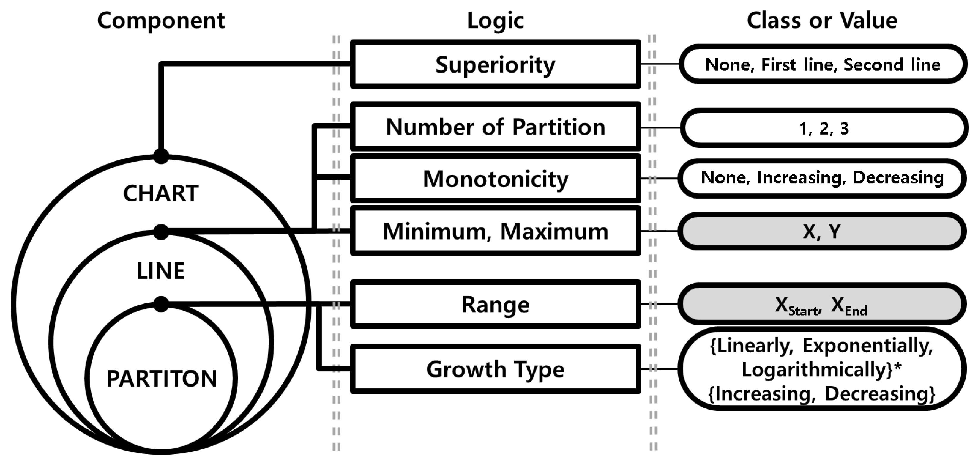
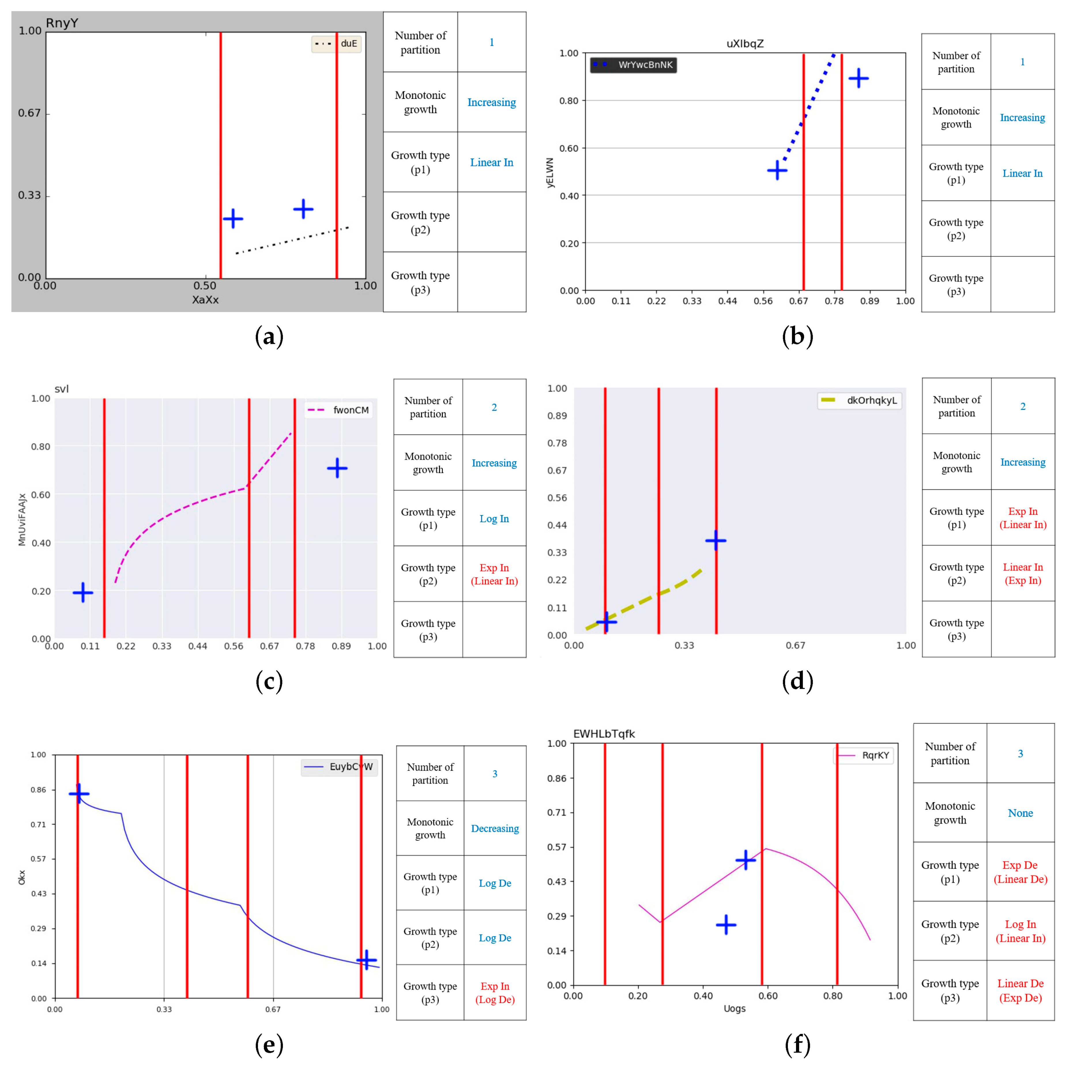
3. Problem Definition for Line Chart Understanding
3.1. Input: A Line Chart Image
- An image has a line chart.
- A chart has at most two lines.
- All lines are continuous and have different colors.
- The origin point is located at the left bottom.
- The range of each axis is [0,1] (a standardized range).
3.2. Output: A Knowledge Template
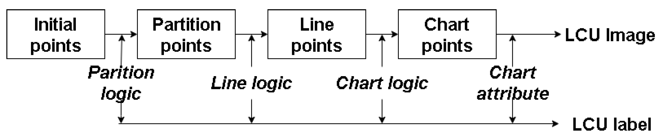
4. Data Generation
4.1. Algorithm to Generate Labeled Data
| Algorithm 1 Generation of synthetic supervised data. |
|
4.2. Detailed Settings for Label Generation
4.3. Detailed Settings for Input Image Generation
5. Experiments
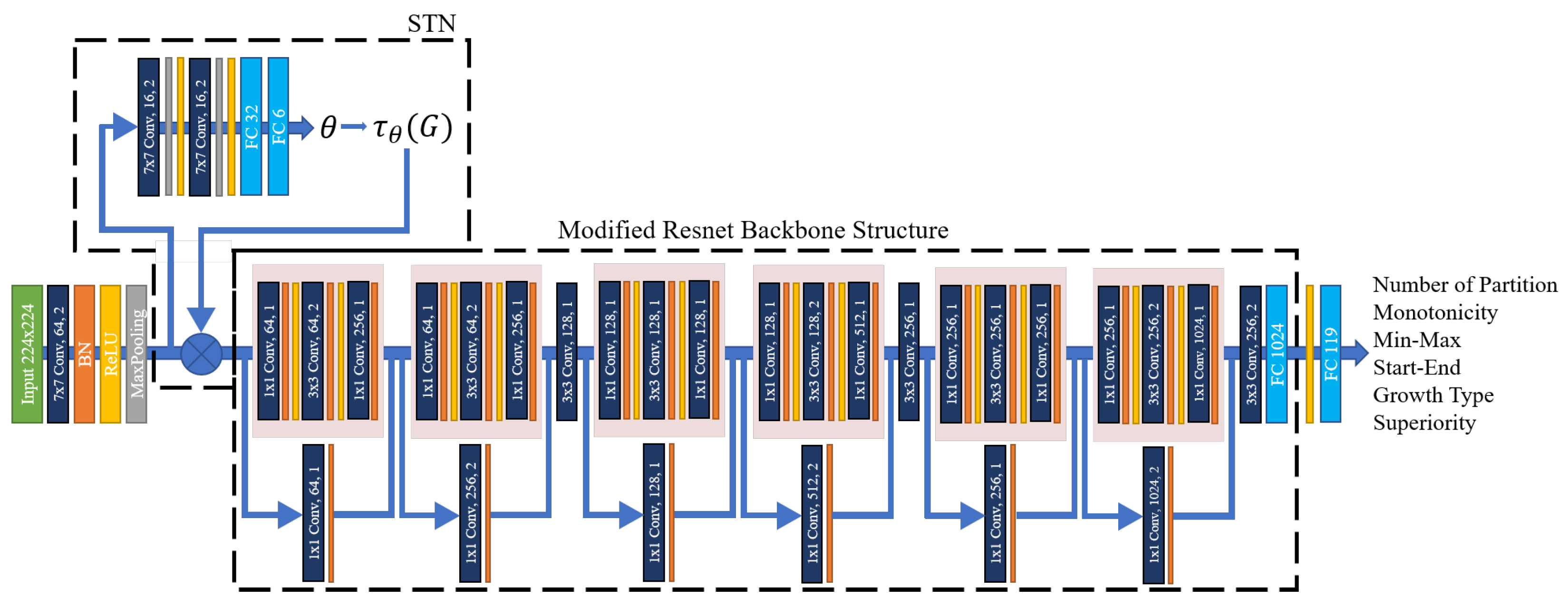
5.1. Model Configuration
5.2. Training Setting
5.3. Evaluation Setting
6. Result and Discussion
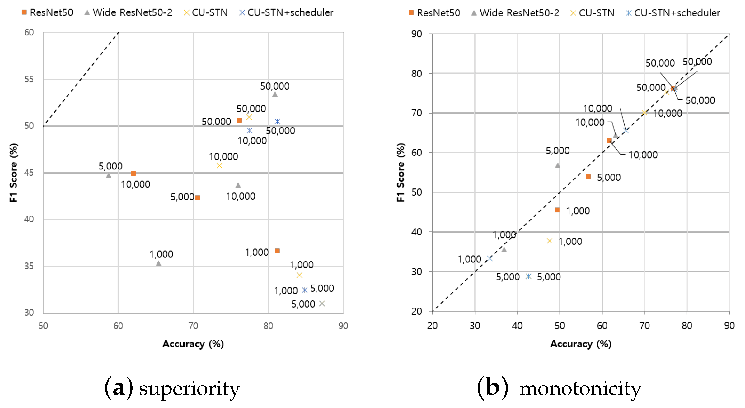
6.1. Quantitative Analysis
6.2. Qualitative Analysis
7. Conclusions
8. Future Works
Author Contributions
Funding
Conflicts of Interest
References
- Balaji, A.; Ramanathan, T.; Sonathi, V. Chart-text: A fully automated chart image descriptor. arXiv 2018, arXiv:1812.10636. [Google Scholar]
- Mishchenko, A.; Vassilieva, N. Chart image understanding and numerical data extraction. In Proceedings of the 2011 Sixth International Conference on Digital Information Management, Melbourne, Australia, 26–28 September 2011; pp. 115–120. [Google Scholar]
- Savva, M.; Kong, N.; Chhajta, A.; Fei-Fei, L.; Agrawala, M.; Heer, J. Revision: Automated classification, analysis and redesign of chart images. In Proceedings of the 24th Annual ACM Symposium on User Interface Software and Technology, Santa Barbara, CA, USA, 16–19 October 2011; pp. 393–402. [Google Scholar]
- Jung, D.; Kim, W.; Song, H.; Hwang, J.i.; Lee, B.; Kim, B.; Seo, J. ChartSense: Interactive data extraction from chart images. In Proceedings of the 2017 Chi Conference on Human Factors in Computing Systems, Denver, CO, USA, 6–11 May 2017; pp. 6706–6717. [Google Scholar]
- Siegel, N.; Horvitz, Z.; Levin, R.; Divvala, S.; Farhadi, A. FigureSeer: Parsing result-figures in research papers. In Proceedings of the Computer Vision—ECCV 2016, Amsterdam, The Netherlands, 11–14 October 2016; pp. 664–680. [Google Scholar]
- Sundermeyer, M.; Alkhouli, T.; Wuebker, J.; Ney, H. Translation modeling with bidirectional recurrent neural networks. In Proceedings of the 2014 Conference on Empirical Methods in Natural Language Processing (EMNLP), Doha, Qatar, 25–29 October 2014; pp. 14–25. [Google Scholar]
- Hutchins, W.J.; Somers, H.L. An Introduction to Machine Translation; Academic Press: London, UK, 1992; Volume 362. [Google Scholar]
- Koehn, P. Statistical Machine Translation; Cambridge University Press: Cambridge, UK, 2009. [Google Scholar]
- Lee, H.; Grosse, R.; Ranganath, R.; Ng, A.Y. Convolutional deep belief networks for scalable unsupervised learning of hierarchical representations. In Proceedings of the 26th Annual International Conference on Machine Learning, Montreal, QC, Canada, 14–18 June 2009; pp. 609–616. [Google Scholar]
- Valueva, M.V.; Nagornov, N.; Lyakhov, P.A.; Valuev, G.V.; Chervyakov, N.I. Application of the residue number system to reduce hardware costs of the convolutional neural network implementation. Math. Comput. Simul. 2020, 177, 232–243. [Google Scholar] [CrossRef]
- Baxter, J. A model of inductive bias learning. J. Artif. Intell. Res. 2000, 12, 149–198. [Google Scholar] [CrossRef]
- Thrun, S. Is learning the n-th thing any easier than learning the first? In Advances in Neural Information Processing Systems; Morgan Kaufmann Publishers: Los Altos, CA, USA, 1996; pp. 640–646. [Google Scholar]
- Kavasidis, I.; Pino, C.; Palazzo, S.; Rundo, F.; Giordano, D.; Messina, P.; Spampinato, C. A saliency-based convolutional neural network for table and chart detection in digitized documents. In Proceedings of the Image Analysis and Processing—ICIAP 2019, Trento, Italy, 9–13 September 2019; pp. 292–302. [Google Scholar]
- Amara, J.; Kaur, P.; Owonibi, M.; Bouaziz, B. Convolutional Neural Network Based Chart Image Classification. In Proceedings of the 25th International conference in Central Europe on Computer Graphics, Visualization and Computer Vision (WSCG 2017), Primavera Congress Center, Plzen, Czech Republic, 29 May–2 June 2017; pp. 83–88. [Google Scholar]
- Siddiqui, S.A.; Malik, M.I.; Agne, S.; Dengel, A.; Ahmed, S. Decnt: Deep deformable cnn for table detection. IEEE Access 2018, 6, 74151–74161. [Google Scholar] [CrossRef]
- Saha, R.; Mondal, A.; Jawahar, C. Graphical Object Detection in Document Images. In Proceedings of the 2019 International Conference on Document Analysis and Recognition (ICDAR), Sydney, Australia, 20–25 September 2019; pp. 51–58. [Google Scholar]
- Huang, W.; Liu, R.; Tan, C.L. Extraction of vectorized graphical information from scientific chart images. In Proceedings of the Ninth International Conference on Document Analysis and Recognition (ICDAR 2007), Curitiba, Brazil, 23–26 September 2007; Volume 1, pp. 521–525. [Google Scholar]
- Ganguly, P.; Methani, N.; Khapra, M.M.; Kumar, P. A Systematic Evaluation of Object Detection Networks for Scientific Plots. arXiv 2020, arXiv:2007.02240. [Google Scholar]
- Huang, W.; Tan, C.L.; Zhao, J. Generating ground truthed dataset of chart images: Automatic or semi-automatic? In Proceedings of the Graphics Recognition. Recent Advances and New Opportunities, Curitiba, Brazil, 20–21 September 2007; pp. 266–277. [Google Scholar]
- Methani, N.; Ganguly, P.; Khapra, M.M.; Kumar, P. PlotQA: Reasoning over Scientific Plots. In Proceedings of the IEEE Winter Conference on Applications of Computer Vision, Snowmass Village, CO, USA, 1–5 March 2020; pp. 1527–1536. [Google Scholar]
- Kahou, S.E.; Michalski, V.; Atkinson, A.; Kádár, Á.; Trischler, A.; Bengio, Y. Figureqa: An annotated figure dataset for visual reasoning. arXiv 2017, arXiv:1710.07300. [Google Scholar]
- Kafle, K.; Price, B.; Cohen, S.; Kanan, C. DVQA: Understanding data visualizations via question answering. In Proceedings of the IEEE Conference on Computer Vision and Pattern Recognition, Salt Lake City, UT, USA, 18–22 June 2018; pp. 5648–5656. [Google Scholar]
- Huang, W. Scientific Chart Image Recognition and Interpretation. Ph.D. Thesis, National University of Singapore, Singapore, 2008. [Google Scholar]
- Cleveland, W.S.; McGill, R. Graphical perception: The visual decoding of quantitative information on graphical displays of data. J. R. Stat. Soc. Ser. A 1987, 150, 192–210. [Google Scholar] [CrossRef]
- Cleveland, W.S.; McGill, R. Graphical perception: Theory, experimentation, and application to the development of graphical methods. J. Am. Stat. Assoc. 1984, 79, 531–554. [Google Scholar] [CrossRef]
- He, K.; Zhang, X.; Ren, S.; Sun, J. Deep residual learning for image recognition. In Proceedings of the IEEE Conference on Computer Vision and Pattern Recognition, Las Vegas, NV, USA, 27–30 June 2016; pp. 770–778. [Google Scholar]
- Zagoruyko, S.; Komodakis, N. Wide residual networks. arXiv 2016, arXiv:1605.07146. [Google Scholar]


| Attribute | Range | |
|---|---|---|
| title | name | up to 10 characters |
| size | [5, 10] (font size) | |
| position | ||
| Axis | label | up to 10 characters |
| label position | ||
| label size | [5, 8] (font size) | |
| label color | ||
| range | [0.0, 1.0] | |
| tick label | up to 10 characters | |
| tick label size | [4, 7] (font size) | |
| tick digit | two decimal places | |
| number of ticks | [3, 12] | |
| Legend | label | up to 10 characters |
| position | ||
| border | ||
| border color | ||
| background | ||
| Line | type | 4 types including sold and dotted type |
| color | ||
| thickness | [1, 4] (line width) | |
| Background | color | |
| grid | ||
| plot area frame |
| Category | Subtask | Number of Subtasks | Type |
|---|---|---|---|
| chart | Superiority | 1 | classification |
| line | Number of Partitions | 2 | classification |
| Monotonicity | 2 | classification | |
| XY-coordinates for Minimum | 4 | regression | |
| XY-coordinates fpr Maximum | 4 | regression | |
| partition | X of start & end for 1 partition case | 4 | regression |
| X of start & end for 2 partition case | 8 | regression | |
| X of start & end for 3 partition case | 12 | regression | |
| Growth Type labels for 1 partition case | 2 | classification | |
| Growth Type labels for 2 partition case | 4 | classification | |
| Growth Type labels for 3 partition case | 6 | classification |
| Subtask | Class | Proportion |
|---|---|---|
| Number of Line | 1 | 49.92% |
| 2 | 50.08% | |
| Number of Partitions | 1 | 33.43% |
| 2 | 33.22% | |
| 3 | 33.35% | |
| Superiority | None | 86.85% |
| Line 1 | 6.77% | |
| Line 2 | 6.38% | |
| Monotonicity | None | 51.27% |
| Increasing | 24.42% | |
| Decreasing | 24.31% | |
| Growth Type | Linear Increasing | 16.74% |
| Linearly Decreasing | 16.7% | |
| Logarithmic Increasing | 16.57% | |
| Logarithmic Decreasing | 16.45% | |
| Exponential Increasing | 16.73% | |
| Exponential Decreasing | 16.82% |
| Dataset | Hyper-Parameter | Value |
|---|---|---|
| Common | batch size | 64 |
| pretrained model | false | |
| Training | validation ratio | 0.5 |
| maximum update step | 500,000 | |
| optimizer algorithm | Adam | |
| optimizer hyperparameter (alpha, beta) | (0.9, 0.999) | |
| learning rate | 0.001 | |
| weight decay | 0 | |
| learning rate scheduler algorithm | ReduceLROnPlateau | |
| scheduler hyperparameter (patience) | min(, 10) | |
| scheduler hyperparameter (factor) | 0.1 | |
| Test | balancing parameters ( monotonicity (None, In., De.) | (0.58, 1.21, 1.21) |
| label weights for superiority (None, Line1, Line2) | (0.11, 1.40, 1.49) |
| Classification Accuracy (%) | Average MSE () | ||||||||||
|---|---|---|---|---|---|---|---|---|---|---|---|
| Growth Type | Part. | Mono. | Super. | Range | Min & | ||||||
| p1 | p2 | p3 | p1 | p2 | p3 | Max | |||||
| ResNet 50 | 1K | 21.47 | 4.26 | 0.78 | 37.24 | 49.41 | 81.19 | 0.65 | 0.53 | 0.45 | 0.70 |
| 5K | 26.27 | 5.60 | 1.48 | 40.24 | 56.72 | 70.61 | 0.55 | 0.50 | 0.44 | 0.69 | |
| 10K | 36.48 | 9.36 | 1.86 | 42.57 | 61.68 | 62.02 | 0.55 | 0.53 | 0.38 | 0.64 | |
| 50K | 76.23 | 49.92 | 25.93 | 60.85 | 76.83 | 76.17 | 0.24 | 0.19 | 0.15 | 0.35 | |
| W-ResNet 50-2 | 1K | 16.95 | 3.09 | 0.58 | 34.76 | 36.87 | 65.37 | 0.53 | 0.39 | 0.30 | 0.70 |
| 5K | 31.92 | 6.65 | 1.63 | 40.87 | 49.49 | 58.71 | 0.46 | 0.40 | 0.32 | 0.50 | |
| 10K | 35.43 | 9.66 | 2.29 | 46.66 | 63.13 | 76.00 | 0.35 | 0.24 | 0.19 | 0.40 | |
| 50K | 78.85 | 52.80 | 30.75 | 64.24 | 77.25 | 80.87 | 0.25 | 0.20 | 0.16 | 0.36 | |
| CU-STN | 1K | 20.02 | 4.18 | 0.39 | 34.22 | 47.60 | 84.14 | 0.55 | 0.35 | 0.27 | 0.64 |
| 5K | 17.15 | 3.22 | 0.43 | 32.58 | 42.59 | 87.16 | 0.48 | 0.32 | 0.22 | 0.63 | |
| 10K | 38.01 | 11.96 | 2.68 | 50.99 | 69.88 | 73.51 | 0.38 | 0.24 | 0.19 | 0.39 | |
| 50K | 71.71 | 46.28 | 21.04 | 62.15 | 75.13 | 77.47 | 0.27 | 0.18 | 0.15 | 0.36 | |
| CU-STN+ scheduler | 1K | 16.26 | 2.93 | 0.74 | 34.52 | 33.51 | 84.87 | 0.49 | 0.33 | 0.23 | 0.63 |
| 5K | 17.15 | 2.97 | 0.23 | 33.28 | 42.59 | 87.16 | 0.47 | 0.32 | 0.22 | 0.62 | |
| 10K | 37.09 | 10.79 | 1.86 | 45.31 | 65.51 | 77.51 | 0.35 | 0.25 | 0.20 | 0.39 | |
| 50K | 69.45 | 37.42 | 13.63 | 59.25 | 76.91 | 81.19 | 0.25 | 0.19 | 0.16 | 0.34 | |
| Classification Accuracy (%) | Average MSE () | |||||||||
|---|---|---|---|---|---|---|---|---|---|---|
| Growth Type | Part. | Mono. | Range | Min & | ||||||
| p1 | p2 | p3 | p1 | p2 | p3 | Max | ||||
| ResNet 50 | 1K | 46.88 | 5.56 | 0.00 | 35.04 | 44.53 | 1.05 | 0.64 | 0.52 | 1.15 |
| 5K | 36.60 | 22.22 | 0.00 | 31.39 | 53.28 | 0.56 | 0.59 | 0.42 | 1.41 | |
| 10K | 50.45 | 16.67 | 7.14 | 26.64 | 69.71 | 0.84 | 0.61 | 0.42 | 0.82 | |
| 50K | 85.71 | 69.44 | 42.86 | 81.02 | 89.05 | 0.49 | 0.15 | 0.13 | 0.69 | |
| W-ResNet 50-2 | 1K | 21.43 | 2.78 | 0.00 | 20.07 | 36.86 | 0.81 | 0.31 | 0.25 | 1.30 |
| 5K | 38.34 | 5.56 | 0.00 | 43.43 | 67.15 | 0.64 | 0.40 | 0.23 | 0.96 | |
| 10K | 65.18 | 19.44 | 7.14 | 28.10 | 82.48 | 0.75 | 0.33 | 0.16 | 0.73 | |
| 50K | 86.61 | 66.67 | 50.00 | 79.93 | 90.15 | 0.49 | 0.20 | 0.14 | 0.58 | |
| CU-STN | 1K | 16.52 | 2.78 | 7.14 | 11.68 | 13.14 | 1.21 | 0.45 | 0.24 | 1.24 |
| 5K | 42.86 | 0.00 | 0.00 | 13.14 | 8.76 | 0.86 | 0.31 | 0.17 | 1.33 | |
| 10K | 59.38 | 25.00 | 0.00 | 50.00 | 84.31 | 0.60 | 0.29 | 0.16 | 0.62 | |
| 50K | 82.14 | 58.33 | 42.86 | 63.14 | 93.07 | 0.51 | 0.20 | 0.13 | 0.56 | |
| CU-STN+ scheduler | 1K | 20.98 | 2.78 | 0.00 | 5.84 | 68.61 | 0.76 | 0.28 | 0.17 | 1.30 |
| 5K | 42.86 | 0.00 | 0.00 | 81.75 | 8.76 | 0.78 | 0.27 | 0.16 | 1.29 | |
| 10K | 50.45 | 19.44 | 0.00 | 22.99 | 70.07 | 0.31 | 0.25 | 0.09 | 0.63 | |
| 50K | 72.77 | 36.11 | 35.71 | 45.98 | 90.15 | 0.61 | 0.21 | 0.18 | 0.62 | |
| Classification Accuracy (%) | Average MSE () | ||||||||||
|---|---|---|---|---|---|---|---|---|---|---|---|
| Growth Type | Part. | Mono. | Super. | Range | Min & | ||||||
| p1 | p2 | p3 | p1 | p2 | p3 | Max | |||||
| ResNet 50 | 1K | 23.79 | 3.19 | 0.41 | 38.65 | 51.35 | 83.75 | 0.68 | 0.57 | 0.44 | 0.71 |
| 5K | 28.23 | 5.98 | 0.41 | 37.43 | 58.78 | 68.75 | 0.61 | 0.55 | 0.46 | 0.71 | |
| 10K | 38.71 | 9.96 | 2.49 | 40.68 | 63.51 | 61.25 | 0.53 | 0.53 | 0.37 | 0.64 | |
| 50K | 74.19 | 55.78 | 19.09 | 62.43 | 76.76 | 78.75 | 0.26 | 0.21 | 0.15 | 0.35 | |
| W-ResNet 50-2 | 1K | 16.53 | 4.38 | 0.00 | 34.86 | 33.92 | 68.75 | 0.56 | 0.43 | 0.30 | 0.71 |
| 5K | 32.26 | 7.17 | 1.24 | 40.68 | 50.95 | 56.67 | 0.49 | 0.43 | 0.32 | 0.48 | |
| 10K | 36.29 | 11.16 | 0.41 | 45.00 | 63.92 | 73.75 | 0.37 | 0.24 | 0.19 | 0.40 | |
| 50K | 75.00 | 49.80 | 26.56 | 64.59 | 77.16 | 80.83 | 0.26 | 0.20 | 0.16 | 0.35 | |
| CU-STN | 1K | 21.37 | 2.39 | 0.41 | 34.73 | 46.49 | 85.00 | 0.58 | 0.36 | 0.27 | 0.64 |
| 5K | 17.74 | 3.98 | 0.00 | 32.84 | 40.81 | 88.33 | 0.52 | 0.34 | 0.24 | 0.62 | |
| 10K | 41.53 | 11.95 | 3.32 | 49.59 | 71.49 | 71.25 | 0.36 | 0.23 | 0.20 | 0.38 | |
| 50K | 68.55 | 52.59 | 20.75 | 63.11 | 76.76 | 78.33 | 0.27 | 0.18 | 0.14 | 0.34 | |
| CU-STN+ scheduler | 1K | 18.95 | 3.19 | 0.83 | 33.38 | 35.00 | 85.42 | 0.54 | 0.35 | 0.24 | 0.63 |
| 5K | 17.74 | 1.59 | 0.00 | 33.51 | 40.81 | 88.33 | 0.51 | 0.34 | 0.24 | 0.62 | |
| 10K | 39.11 | 9.16 | 1.66 | 45.68 | 66.49 | 76.25 | 0.36 | 0.25 | 0.20 | 0.37 | |
| 50K | 70.16 | 37.05 | 16.18 | 58.92 | 77.84 | 80.42 | 0.26 | 0.19 | 0.16 | 0.33 | |
| Classification Accuracy (%) | Average MSE () | ||||||||||
|---|---|---|---|---|---|---|---|---|---|---|---|
| Growth Type | Part. | Mono. | Super. | Range | Min & | ||||||
| p1 | p2 | p3 | p1 | p2 | p3 | Max | |||||
| ResNet 50 | 1K | 27.03 | 6.72 | 2.23 | 41.53 | 50.84 | 85.35 | 0.49 | 0.44 | 0.40 | 0.65 |
| 5K | 34.24 | 9.12 | 2.35 | 42.16 | 61.84 | 85.90 | 0.54 | 0.37 | 0.36 | 0.61 | |
| 10K | 43.67 | 12.60 | 2.82 | 45.41 | 69.36 | 86.70 | 0.38 | 0.31 | 0.24 | 0.45 | |
| 50K | 75.93 | 47.70 | 27.79 | 61.01 | 76.18 | 86.45 | 0.24 | 0.20 | 0.15 | 0.35 | |
| W-ResNet 50-2 | 1K | 22.39 | 5.53 | 2.28 | 42.56 | 51.23 | 84.98 | 0.37 | 0.27 | 0.25 | 0.52 |
| 5K | 35.69 | 9.59 | 2.18 | 44.07 | 64.21 | 85.90 | 0.45 | 0.34 | 0.26 | 0.48 | |
| 10K | 42.53 | 13.00 | 2.74 | 46.89 | 70.17 | 86.66 | 0.35 | 0.24 | 0.19 | 0.39 | |
| 50K | 77.02 | 52.49 | 32.30 | 63.07 | 76.59 | 87.28 | 0.24 | 0.20 | 0.17 | 0.37 | |
| CU-STN | 1K | 24.71 | 4.74 | 2.30 | 39.71 | 52.13 | 84.98 | 0.41 | 0.30 | 0.25 | 0.58 |
| 5K | 18.44 | 4.17 | 0.97 | 34.14 | 42.90 | 85.90 | 0.48 | 0.32 | 0.22 | 0.62 | |
| 10K | 477 | 12.24 | 2.70 | 49.25 | 72.41 | 86.85 | 0.38 | 0.25 | 0.20 | 0.38 | |
| 50K | 73.37 | 45.74 | 24.13 | 60.75 | 75.64 | 87.63 | 0.26 | 0.19 | 0.14 | 0.35 | |
| CU-STN+ scheduler | 1K | 285 | 4.35 | 0.77 | 37.00 | 48.25 | 84.98 | 0.46 | 0.31 | 0.25 | 0.63 |
| 5K | 17.24 | 3.14 | 1.21 | 36.51 | 42.90 | 85.90 | 0.48 | 0.32 | 0.22 | 0.62 | |
| 10K | 38.98 | 11.11 | 2.62 | 44.94 | 66.36 | 86.66 | 0.36 | 0.26 | 0.20 | 0.39 | |
| 50K | 72.78 | 42.01 | 18.20 | 60.41 | 75.78 | 88.17 | 0.25 | 0.19 | 0.15 | 0.34 | |
Publisher’s Note: MDPI stays neutral with regard to jurisdictional claims in published maps and institutional affiliations. |
© 2021 by the authors. Licensee MDPI, Basel, Switzerland. This article is an open access article distributed under the terms and conditions of the Creative Commons Attribution (CC BY) license (http://creativecommons.org/licenses/by/4.0/).
Share and Cite
Sohn, C.; Choi, H.; Kim, K.; Park, J.; Noh, J. Line Chart Understanding with Convolutional Neural Network. Electronics 2021, 10, 749. https://doi.org/10.3390/electronics10060749
Sohn C, Choi H, Kim K, Park J, Noh J. Line Chart Understanding with Convolutional Neural Network. Electronics. 2021; 10(6):749. https://doi.org/10.3390/electronics10060749
Chicago/Turabian StyleSohn, Chanyoung, Heejong Choi, Kangil Kim, Jinwook Park, and Junhyug Noh. 2021. "Line Chart Understanding with Convolutional Neural Network" Electronics 10, no. 6: 749. https://doi.org/10.3390/electronics10060749
APA StyleSohn, C., Choi, H., Kim, K., Park, J., & Noh, J. (2021). Line Chart Understanding with Convolutional Neural Network. Electronics, 10(6), 749. https://doi.org/10.3390/electronics10060749