Stereo Matching with Spatiotemporal Disparity Refinement Using Simple Linear Iterative Clustering Segmentation

Abstract

Stereo matching is a challenging problem, especially for computer vision, e.g., three-dimensional television (3DTV) or 3D visualization. The disparity maps from the video streams must be estimated. However, the estimated disparity sequences may cause undesirable flickering errors. These errors result in poor visual quality for the synthesized video and reduce the video coding information. In order to solve this problem, we here propose a spatiotemporal disparity refinement method for local stereo matching using the simple linear iterative clustering (SLIC) segmentation strategy, outlier detection, and refinements of the temporal and spatial domains. In the outlier detection, the segmented region in the initial disparity is used to distinguish errors in the binocular disparity. Based on the color similarity and disparity difference, we recalculate the aggregated cost to determine adaptive disparities to recover the disparity errors in disparity sequences. The flickering errors are also effectively removed, and the object boundaries are well preserved. Experiments using public datasets demonstrated that our proposed method creates high-quality disparity maps and obtains a high peak signal-to-noise ratio compared to state-of-the-art methods.

1. Introduction

Over the past several decades, disparity estimation is a problem in stereo vision, which has been investigated, and is still an active research topic in the field of computer vision [1]. It is a fundamental technology for the next-generation of network services to synthesize virtual viewpoints, including 3DTV, multiview video, free-view video, and virtual reality operations.

Stereo matching is an important vision problem that estimates the disparities in a given stereo image pair. Many stereo matching techniques have been proposed, which could be categorized as either global or local methods [2]. The global methods produce more accurate disparity maps, which are typically derived from an energy minimization framework that allows for the express integration of disparity smoothness constraints, and are thus able to regularize the solution in weakly textured areas. However, as a result of minimization, they use an iterative strategy or graph cuts, which require a high computing cost. These methods are often quite slow, and thus unsuitable for processing a large amount of data. In contrast, local methods compute the disparity value by optimizing a matching cost, which compares the candidate target pixels and reference pixels while simultaneously considering the neighboring pixel information in a support window [3]. Local methods, which are typically built upon the winner-takes-all (WTA) framework [4,5,6], have the lowest computational costs and are suitable for implementation on parallel graphics processers. In the WTA framework, local stereo methods consider a range of disparity hypotheses and compute a cost volume using various pixel-wise dissimilarity metrics between the reference image and the matched image at every considered disparity value. The final disparities are selected from the cost volume by going through its values and selecting the disparities associated with the minimum matching costs for every pixel of the reference image. Hence, considering the computational cost, we used a local method with the WTA strategy in this study.

Adaptive-weight methods, iteratively updated support windows, and support weights [4,6,7] have been used to find a support window and support weight for each pixel, while fixing the shape and size of a local support window. Although these methods can obtain excellent results using adaptive-weight algorithms, pixel-wise support weight computation is very time-consuming. De-Maeztu et al. [8] proposed a local stereo matching algorithm inspired by anisotropic diffusion to reduce the computational requirements. However, the results were similar to those of the adaptive-weight method. Kowalczuk et al. [6] combined temporal and spatial cost aggregations to improve the accuracy of stereo matching in video clips using iterative support weights.

Richardt et al. [9] extended the dual-cross-bilateral grid method to the time dimension by applying a filter to the temporally adjacent depth images to smooth out the depth change, and presented its real-time performance using the adaptive support weights algorithm [4]. However, the results were less accurate than those of the adaptive-weight algorithm [4].

Vretos and Daras [10] used a temporal window to calculate the disparity and enforce its temporal consistency on outliers, where the color remains within a certain distribution. This method used a range of frames to calculate the disparity at a pixel for a frame. However, object occlusion and motion will affect the determination of frame interval and disparity calculation in the specific temporal window. This causes the loss of disparity values of some object boundaries. Liu et al. [11] proposed a spatiotemporal consistency enhancement method based on a guided filter in the spatial domain to reduce noises and inconsistent pixels, along with an adaptive filter in the temporal domain to improve the temporal consistency. Although this method could reduce noises and transient errors, the disparity maps were blurred after performing these filtering operations.

Jung et al. [12] proposed a boundary-preserving stereo matching method to improve the fidelity of error disparities. This approach used segmentation-based disparity estimation, and the classification information of the certain and uncertain regions was used to adjust the disparity map in the support window. The initial disparity maps were obtained using the segmentation method. However, the noises and occlusion will disturb the segmentation process and reduce the initial disparity quality.

Me et al. [13] used a four-mode census transform stereo matching method to improve the matching quality. This method used bidirectional constraint dynamic programming and relative confidence plane fitting. In a census window, the matching cost is determined by computing the Hamming distance of two bit strings. However, the matching cost computation in the window-based census transform is sensitive to all of the pixels in the window and noises, which will reduce the matching accuracy.

Zhan et al. [14] proposed an image-based stereo matching approach that used the combined matching cost and multistep disparity refinement to improve the local stereo matching algorithm. This method was used for image-guided and filter-based guidance images to enhance the raw stereo images and improve the existing local stereo matching algorithm. The final disparity map removed the outliers using the combined matching cost, which included the double-RGB gradient, census transform, image color information, and a sequence of refinement sets.

Yang et al. [7] proposed a dynamic scene-based local stereo-matching algorithm that integrated a cost filter with motion flow in dynamic video clips. This method used the motion flow to calculate a suitable support weight for estimating the disparity and obtained an accurate stereo-matching result. However, a problem with occlusion will generate discontinuities in some objects. Thus, using the motion flow may produce an incorrect matching when the object was rotated, making it impossible to obtain a suitable weight. Some stereo matching algorithms based on the modified cost aggregation have been reported [15,16,17,18,19,20].

Although the stereo matching method provides excellent matching results for the two image pairs, there are still some complicated problems with stereo matching, such as object occlusion and flickering artifacts. Object occlusion, where there are no corresponding pixels to be captured, is a serious problem that could cause the stereo matching algorithm to be ineffective at finding the correct pixels. Thus, it will produce incorrect disparity values in the occluded regions. In addition, the problem of flickering artifacts usually occurs in disparity sequences generated by a stereo matching method as a result of inconsistent disparity maps. These flickers will significantly reduce the subjective quality of a video clip. Simultaneously, the incorrect disparity values would cause visual discomfort in the human eye, especially when they are used for synthesizing a virtual view in depth-image-based rendering (DIBR). To address this issue, we propose a strategy based on the spatiotemporal domain to reduce the inconsistent disparities and to refine the disparity map in a video clip. The main contribution of our proposed method is to improve the inconsistent disparities and reduce flickering errors in the estimated disparity sequences for the synthesized video. The advantages of this method are as follows. First, the outliers can be detected and removed using the superpixel-based segmentation method. Second, the disparity refinement is achieved using our proposed technique in the temporal and spatial domains. In the temporal domain, we propose the method to improve the cost aggregation based on segmentation, color difference, and disparity difference and then to refine the outliers in frames. In the spatial domain, the rest of disparity errors of each frame can be further refined based on refinement within superpixel bounds, propagation mechanism, and filtering. Finally, our proposed method is easy to implement and an efficient technique.

2. Preliminary Techniques

In this section, we briefly describe the techniques related to our proposed approach.

2.1. Cross-Based Local Stereo Matching

In recent years, a local stereo matching method has usually been used to generate a disparity map. A well-known cross-based local stereo matching proposed by Zhang et al. [5] based on a shape-adaptive support region is an efficient and easy method. The main goals are to create a local upright cross for the anchor pixel and then construct an adaptive support region. This local support region should only contain the neighboring pixels with the same depth as the anchor pixel under consideration.

First, we construct a local cross support region for a pixel using the color information. We define pixel p within the shape-adaptive support region and then compute the cost aggregation based on a WTA strategy corresponding to each pixel, as shown in Figure 1. Using a variable cross support region instead of a fixed size for each pixel can efficiently reduce the computational complexity.

Cross-based aggregation proceeds by a two-step process, as shown in Figure 1. In the first step, an upright cross is constructed for each pixel. The support region of pixel p is modeled by merging the horizontal arms of the pixels (q for example) lying on the vertical arms of pixel p, as shown in Figure 1b. As per [5], there is an alternative, merging vertical arms of pixels lying on the horizontal arms of pixels p. In the second step, the aggregated cost based on the WAT strategy in the support region is computed within two passes. The first pass sums up the matching costs horizontally and stores the intermediate results; the second pass then aggregates the intermediate results vertically to obtain the final cost. Aggression or finite summation was used for the matching cost function while Figure 1 referred to horizontal or vertical aggregation. More details about the method can be found in [5].

2.2. SLIC Segmentation and Merging

The SLIC segmentation method was proposed by [21]. It groups the pixels of an image into perceptually meaningful atomic regions that can be used to replace the rigid structure of the pixel grid using a k-means clustering approach. These grouped pixels are called superpixels. This method can adhere to the boundaries very well. The only parameter in the SLIC segmentation method is $n_0$, which is the desired number of superpixels of approximately equal size. The choice of this parameter $n_0$ is depending on the users for the experiments.

The SLIC segmentation method adopts the CIELAB color space. The clustering procedure begins with an initialization step, where the $n_0$ initial cluster centers $C_i={\left[l_i,a_i,b_i,x_i,y_i\right]}^T$ are sampled on a regular grid, spaced S pixels apart. To generate superpixels of roughly equal size, the grid interval is $S=\sqrt{\raisebox{1ex}{$N$}\!\left/ \!\raisebox{-1ex}{$n_0$}\right.}$, where N represents the number of pixels for an image. The SLIC algorithm [21] obtains the desired number of clusters with size $\frac{N}{n_0}$. Additionally, in order to avoid centering a superpixel on an edge or a noisy pixel, the centers are moved to seed locations corresponding to the lowest gradient positions in 3 × 3 neighborhoods. It is known that an edge or a noisy pixel is often positioned on a pixel point with the largest gradient variance. Therefore, selecting the lowest gradient pixel point when positioning the center of a superpixel can efficiently reduce the chance of seeding a superpixel with an edge or a noisy pixel.

After performing the SLIC segmentation, we can obtain the number of desired clusters that adhere to the boundaries of objects. However, some neighboring clusters that belong to the same object are segmented into different clusters. In order to obtain a greater advantage and more useful segmented information, we further merge some neighboring clusters into a larger cluster when the average color difference between neighboring clusters i and j, is less than a threshold ($T_s$). Given two adjacent superpixels (i.e., “clusters”) clustered at pixels i and j, respectively, denoted by $S{E}_c(i)=\left\{I_c(p)\left|p=\left(x_p,y_p\right)\in S_i,c\in \left\{R,G,B\right\}\right.\right\}$, where $S_i$ represents the set of pixel locations and $\left(x_p,y_p\right)$ representing coordinates of pixel p in a two-dimensional (2D) space, in the superpixel i with a total number of pixels, $N_{s_i}=\mathrm{card}(S_i)$ the average color difference between neighboring clusters i and j is denoted as follows.

$$AveCD(i,j)=\frac{1}{3}\left|\frac{{\displaystyle {\sum }_{c\in \left\{R,G,B\right\}}{\displaystyle {\sum }_{p\in S_i}{I}_c(p)}}}{N_{S_i}}-\frac{{\displaystyle {\sum }_{c\in \left\{R,G,B\right\}}{\displaystyle {\sum }_{p\in S_j}{I}_c(p)}}}{N_{S_j}}\right|,$$

(1)

It is noted that symbol “card(●)” denotes the cardinality operator. This threshold ($T_s$) is set to 8, which is a value obtained through experimentation. Based on our experiments, if this threshold is greater than the specified value, the boundary information of clusters will be lost which will impact the following inpainting process. Figure 2 shows an example of the SLIC segmented results and merging.

3. Proposed Method

This section describes the proposed method, which includes simple linear iterative clustering (SLIC) segmentation and merging, and temporal and spatial refinements. Figure 3 illustrates the flowchart of the proposed system. The procedures are described in detail in the following subsections.

3.1. Outlier Detection Based on Disparity Variation

The initial disparity of each pixel according to the map calculated by the cross-based local stereo matching [5] contains many outliers. In order to detect these outliers, we here use the consistency of the disparity variation under the same cluster to label the inconsistent pixels in the current frame. These inconsistent pixels are marked as outliers. Due to the disparity variation, one cluster may include many disparity values, which will cause inconsistent disparity values within the same cluster. Hence, we estimate the variation of the disparity values in the same cluster to detect the inconsistent pixels. First, all of the pixels in the disparity map are given different initial labels. Given a pixel $p=\left(x_p,y_p\right)\in S_p$ with label $l_p$, for every pixel $q=\left(x_q,y_q\right)\in S_P$, a constraint is enforced on its labeling as follows.

$$l_q=\left\{\begin{array}{ll}{l}_p,\hfill & \mathrm{if} \left|d\left(p\right)-d\left(q\right)\right|<{\alpha }_e,\hfill \\ l_q,\hfill & \mathrm{otherwise},\hfill \end{array}\right.$$

(2)

where $S_p$ is the cluster containing pixel p, $d\left(\cdot \right)$ denotes the disparity corresponding to a pixel, and ${\alpha }_e$ is a threshold. The symbol $\left|\cdot \right|$ denotes the absolute value. In a cluster, there exist many pixels, there might be different labels. In that cluster, the pixels with the label shown most frequently denote as a target. In the target, the disparity shown most frequently denotes the correct disparity. This value is found from those pixels with the same label shown most frequently. Additionally, the rest of the pixels are denoted as the outliers of the cluster.

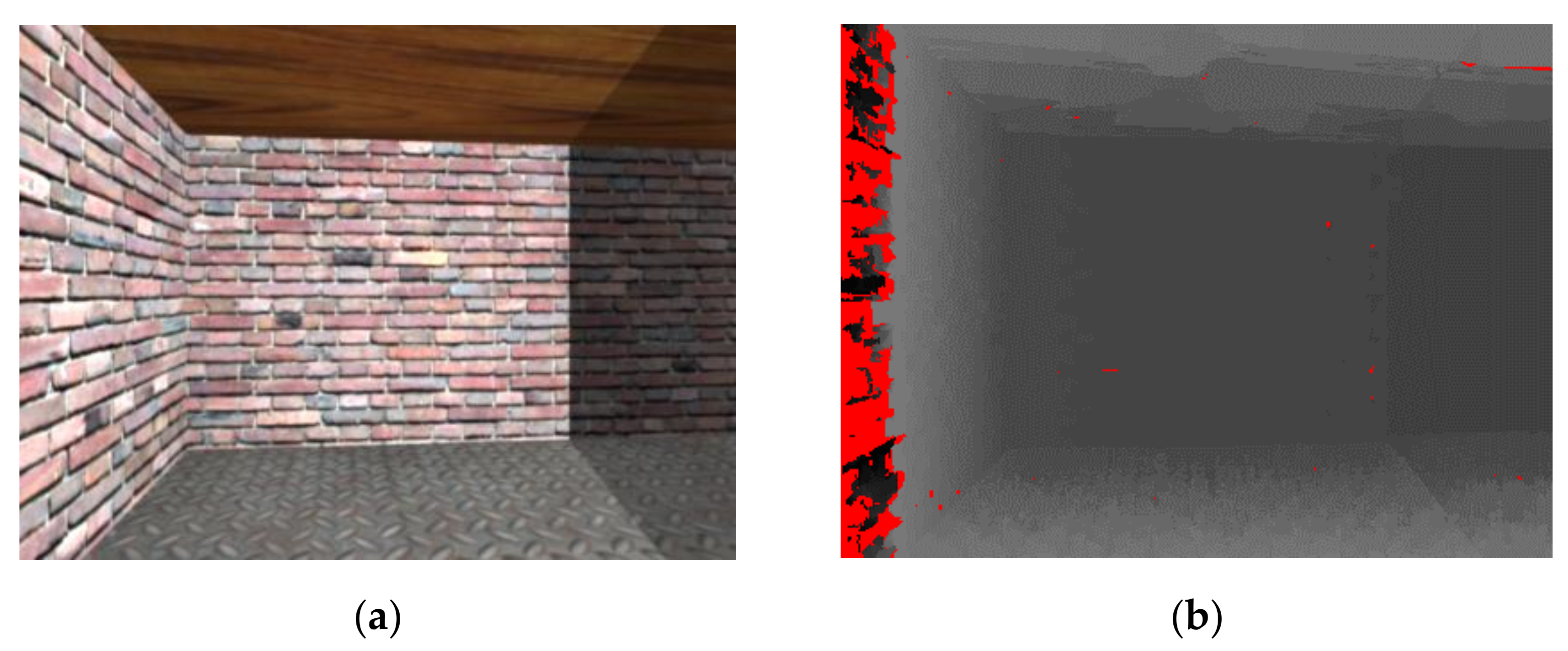
However, the leftmost or rightmost disparities of the disparity sequences may cause serious disparity errors because they do not have related information in the left or right image. Thus, these pixels have zero values. In other words, the corresponding region at the leftmost or rightmost of the disparity map cannot be matched. Hence, the disparity value is zero, which indicates an error. We use the following procedures to detect the disparity errors positioned at the leftmost or rightmost of the disparity sequences. First, we detect segmented regions that include disparities with a value of zero in the leftmost or rightmost region. Then, we use the characteristic of a disparity variation from an endpoint to inner point and compute the average disparity of the segmented region. If the average disparity is less than a threshold ($T_{\mathrm{d}}$ = 4), this segmented region is labeled as having disparity error. After performing the above procedures, the disparity errors generated at the leftmost or rightmost of a disparity map can be reduced.

The detected outliers are recorded on the disparity map for the left view, as shown in Figure 4. In Figure 4, the red points are the outliers. In other words, these outliers are regarded as disparity error points on the disparity map with the left view and must be refined.

3.2. Disparity Refinement in Temporal Domain

After detecting the outliers, we can determine the outliers in each frame within a video clip. When the camera or captured objects in the scene involve slow motion, the disparity of an object cannot show a dramatic change in a short period of time. In addition, an occlusion will cause a disparity with a great change in the background, which will result in disparity errors. However, a dramatic change may be caused by the appearance of another object. Hence, this approach will refine these disparity errors, whether they are caused by the appearance of another object or an occlusion.

These errors must be removed and refined in the disparity map. In our approach, the refining procedures are divided into two phases: refining in the temporal domain and in the spatial domain. The system design uses an object-based strategy.

We combine the segmentation information, region movement, color difference, and disparity difference to achieve the refinement in the temporal domain at this stage. We simply use the previous frame and its corresponding information to perform the refinement. The details of the procedures at this stage are described in the following.

3.2.1. Searching for Matching Point in Previous Frame

First, we need to search for the matching positions in the previous frame corresponding to the outliers in the current frame. Assuming that a given pixel, p, is in the current frame (at time t), $I_{n_f}$, with $p\in R_p$ where $R_p$ denotes a cluster as a result of the SLIC segmentation and merging, the candidate pixel, $p^{\prime }$, is from a given search window of 11 × 11 pixels in the previous fame denoted by $W_s$, i.e., $p^{\prime }\in W_s$, with its matching window to $R_p$ denoted by $R_{p^{\prime }}$, the best matching point, $p\ast$, in the previous frame (at time t−1) $I_{(n_f-1)}$, to pixel p of the current frame, $I_{n_f}$, is defined as follows,

$$p\ast =\arg \underset{p^{\prime }\in W_s}{\min }J\left(p,p^{\prime }\right),$$

(3)

where the cost function, $J\left(p,p^{\prime }\right)$, is composed of color matching, $J_c\left(p,p^{\prime }\right)$, and disparity matching cost, $J_d\left(p,p^{\prime }\right)$, and is defined as

$$J\left(p,p^{\prime }\right)=J_c\left(p,p^{\prime }\right)+\beta \times J_d\left(p,p^{\prime }\right),$$

(4)

$\beta$ is a weighting parameter,

$$J_c\left(p,p^{\prime }\right)=\frac{{\displaystyle {\sum }_{p_{n_f}\in R_p,p_{(n_f-1)}\in R_{p^{\prime }},}\left(\frac{1}{3}\left({\displaystyle {\sum }_{c\in \left\{R,G,B\right\}}\left|I_{n_f.c}(p_{n_f})-I_{n_f-1,c}(p_{(n_f-1)})\right|}\right)\right)}}{\mathrm{card}(R_p)},$$

(5)

symbol “card(●)” denotes the cardinality operator, $p_{n_f}$ and $p_{(n_f-1)}$ are indexes to matching windows in frames $I_{n_f}$ and $I_{(n_f-1)}$, respectively.

$$J_d(p,p^{\prime })=\frac{{\displaystyle {\sum }_{p_{n_f}\in R_p,p_{(n_f-1)}\in R_{p^{\prime }},}{J}_{pd}\left(p_{n_f},p_{(n_f-1)}\right)}}{N_d(R_p,R_{p^{\prime }})},$$

(6)

$J_{pd}\left(p_{n_f},p_{(n_f-1)}\right)$ denotes the pixel level disparity matching cost and is defined, for $p_{n_f}\in R_p$, $p_{(n_f-1)}\in R_{p^{\prime }}$, by

$$J_{pd}\left(p_{n_f},p_{(n_f-1)}\right)=\left\{\begin{array}{cc}\left|d(p_{n_f})-d(p_{(n_f-1)})\right|,& \mathrm{if} E_{p_{n_f}}=false \mathrm{and} E_{p_{(n_f-1)}}=false,\\ 0,& \mathrm{otherwise}.\end{array}\right.$$

(7)

$N_d(R_P,R_{P^{\prime }})$ denotes the number of points that possess correct disparities in the matching windows in frames $I_{n_f}$ and $I_{(n_f-1)}$, and is defined by

$$N_d(R_p,R_{p^{\prime }})={\displaystyle {\sum }_{p_{n_f}\in R_p,p_{(n_f-1)}\in R_{p^{\prime }},}{D}_E\left(p_{n_f},p_{(n_f-1)}\right)},$$

(8)

with $D_E\left(p_{n_f},p_{(n_f-1)}\right)$ identifying pixels with correct disparities in candidate matching region and defined as

$$D_E\left(p_{n_f},p_{(n_f-1)}\right)=\left\{\begin{array}{cc}1,\hfill & \mathrm{if} E_{p_{n_f}}=false \mathrm{and} E_{p_{(n_f-1)}}=false,\\ 0,\hfill & \mathrm{otherwise},\end{array}\right.$$

(9)

where $E_{p_{n_f}}$ denotes the disparity of point p in the current frame, $I_{n_f}$, whether there is an error or not. Additionally, $E_{p_{(n_f-1)}}$ denotes the disparity of point p in the previous frame, $I_{(n_f-1)}$, whether there is an error or not. Hence, $E_{p_{n_f}}=false$ means that the disparity of point p is correct, and the disparity of point p in the previous frame is correct. According to Equation (3), the best matching point in the previous frame corresponding to the outlier in the current frame can be obtained. 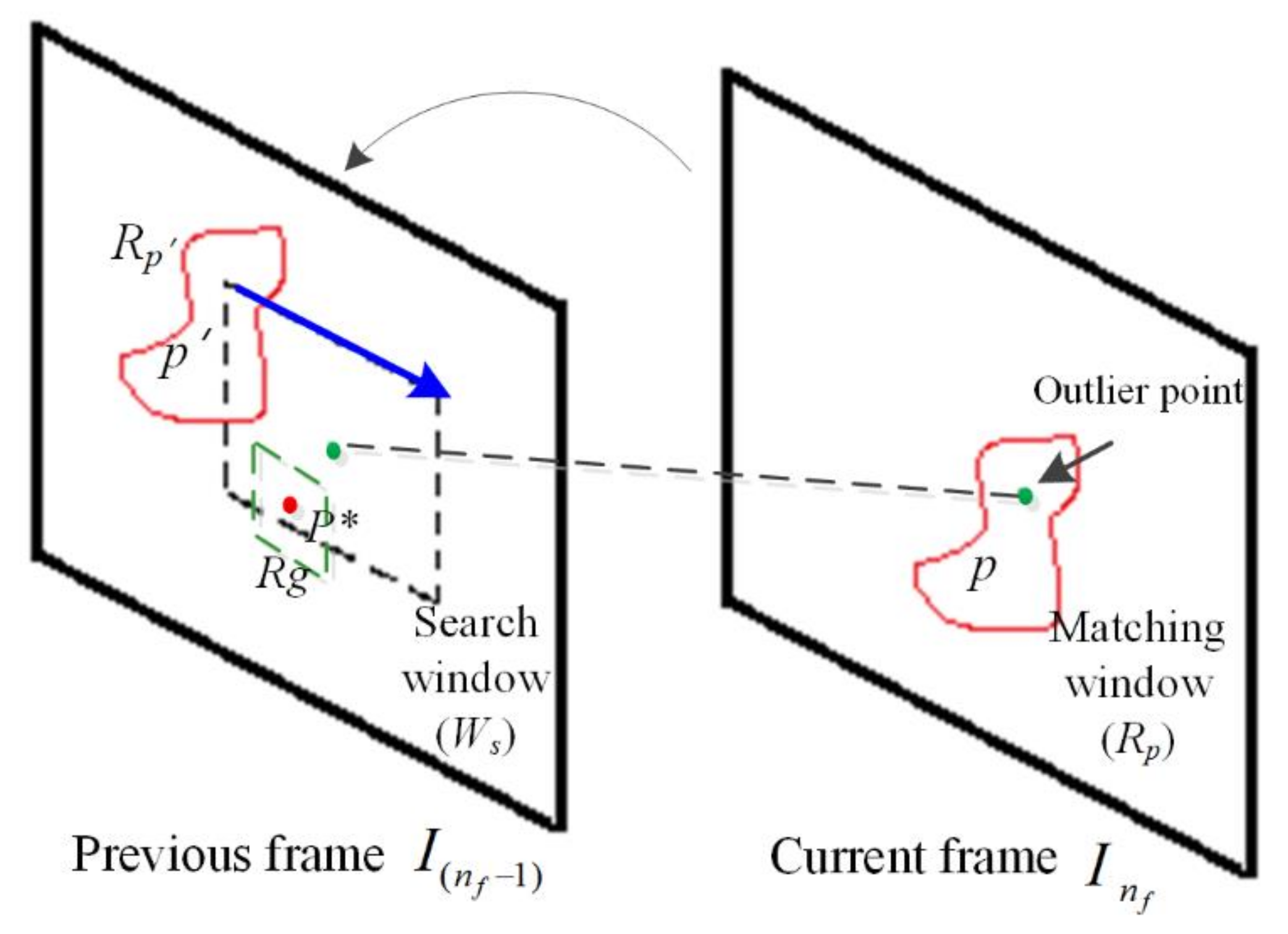Figure 5 shows the profile of the matching operation.

Afterward, we further compute and record the displacement of the coordinates of the matching point. The displacement of the coordinates of p and p* is computed as follows:

$$\begin{array}{l}{D}_x(p)=x_p-x_{p\ast },\\ D_y(p)=y_p-y_{p\ast }.\end{array}$$

(10)

Based on the displacement information, we can more rapidly obtain the matching points of other outliers within the same segmented region. This is because they are clustered in the same region.

Hence, if we search for other matching points in the previous frame corresponding to any disparity errors in the same segmented region for the current frame, we can decide whether the displacement information belonging to the same cluster is recorded or not. Based on the displacement information, it is easier and quicker to find the matching point corresponding to the disparity error.

3.2.2. Disparity Refinement of Outliers

In terms of disparity refinement, based on the matching result in the previous process, we can obtain the matching point corresponding to the outlier. However, this matching point may not have the correct disparity. In order to avoid matching the error disparity, we use the color difference between point p in the current frame I and the neighborhood pixels of matching point p* in the previous frame $I^{pre}$ to select the appropriate matching point. The selection of the appropriate matching point is computed using Equations (11) and (12):

$$k=\arg {\min }_{p\ast \in Rg}\left({\displaystyle \sum _{c\in \left\{R,G,B\right\}}\left|I_c(p)-I_c^{pre}(p\ast )\right|}\right),$$

(11)

where Rg is a 3 × 3 region with center point p*, as shown in Figure 5.

After the computation using Equation (11), we further determine whether the disparity of point k is right or not, and then compute the color difference between point k and point p. In order to maintain temporal consistency for the pixels in the temporal sequence, a threshold (${\alpha }_t$) is used to estimate whether the colors of the pixels remain within a certain distribution. When the color difference is less than a threshold (${\alpha }_t$) and the disparity of point k is correct, the disparity error will be replaced by the disparity of point k. The disparity refinement of the outliers in the temporal domain is expressed as follows:

$$d_T(p)=\left\{\begin{array}{ll}d(k),\hfill & \mathrm{if} E_k=false \& {\displaystyle \sum _{c\in \left\{R,G,B\right\}}\left|I_c(p)-I_c^{pre}(k)\right|}<{\alpha }_t, \hfill \\ d(p),\hfill & \mathrm{otherwise},\hfill \end{array}\right.$$

(12)

where $d\left(p\right)$ and $d\left(k\right)$ denote the disparities of pixel p and pixel k, respectively. $E_k$ denotes the disparity of point k at time t-1, whether there is an error or not. Hence, $E_k=false$ means that the disparity of pixel k is correct. At the same time, the color difference between pixel p at time t and pixel k at time t-1 is less than a threshold (${\alpha }_t$). Thus, the disparity of pixel p in the current frame is replaced by the disparity of pixel k.

After refining the disparities of the outliers at time t in the temporal domain, the refined current frame will be reused for the refinement in the next frame. In other words, the correct disparities for the object in the current frame can propagate to the following frames and be used to refine the same object under the specified camera lens motion.

3.3. Disparity Refinement in Spatial Domain

After performing the refinement in the temporal domain, a large number of the disparity errors were refined. However, some errors still exist in the temporal sequence. Hence, the rest of the errors will be refined in the spatial domain.

3.3.1. Refinement within Superpixel Bounds

Based on the SLIC segmentation and merging, we will search the correct disparities to refine the rest disparities of error values using pixel-based processing of each frame. We compute the color differences between the pixels with the disparity error and the candidate pixels with the correct disparities, which are segmented into the same cluster. The disparity of a pixel with a minimum color difference is used to replace the disparity error of a pixel.

In order to refine the rest of the disparity errors in the spatial domain, first, given a pixel, p, of disparity image in a segmented region $N_s$, i.e., $p\in N_s$, and a 37 × 37 search region denoted by $S_s$, a truth table for the candidate pixels representing correct disparity within the search region $S_s$ can be formulated for $j\in S_s$,

$${\mathrm{T}}_{c_p}[j]=\left\{\begin{array}{ll}true,\hfill & \mathrm{if} E_j=false \&{\displaystyle {\sum }_{c\in \left\{R,G,B\right\}}\left|I_c(p)-I_c^{pre}(j)\right|<{\alpha }_s\&} p,j \in N_s,\hfill \\ false,\hfill & \mathrm{otherwise},\hfill \end{array}\right.$$

(13)

where $E_j$ denotes that the disparity of pixel j is error. $E_j=false$ denotes that the disparity of pixel j is correct. $a_s$ is a threshold for the color difference between point p and point j. Based on the segmentation process, if any two pixels in the spatial domain are segmented into the same cluster, and the color difference between these two pixels is less than a threshold, these points will act as the candidate pixels for refining.

Next, the best candidate pixel among all of the candidate pixels denoted by $S_c$ is selected as follows:

$$b=\underset{h\in S_c \forall {\mathrm{T}}_{c_p}[h]=true}{\arg \min }{\displaystyle {\sum }_{c\in \left\{R,G,B\right\}}\left|I_c(p)-I_c(h)\right|},$$

(14)

and disparity value at p is replaced by that at b as follows,

$$d_s(p)=d(b).$$

(15)

Based on Equation (14), we can obtain the best pixel b, and the disparity of pixel p is replaced by the disparity of pixel b.

3.3.2. Propagation from Horizontal Lines

After performing the disparity refinement of the outliers in the spatial domain and temporal domain, the boundaries of objects may look uneven, a few outliers may not have been corrected, or spatial noises exist in the frame. Thus, we use the following procedures to process the rest of the outliers.

The recovering procedures are described as follows. We use the propagation method in the horizontal direction for an outlier to further recover the disparity error. Assume that pixel p is an outlier. We search for pixels with the correct disparities along the left arm and right arm for equal distances. This search procedure ends when the first correct disparity derived from the left arm or right arm is obtained. Then, we compute the color differences between the outlier and these pixels within the two arms and obtain the maximum color difference for the two arms. The maximum color difference for the two arms is computed as follows:

$$\begin{array}{l}c{m}_l(p,i)={\max }_{sp\in ar{m}_l(p,i)}{\displaystyle \sum _{c\in [R,G,B]}\left|I_c(p)-I_c(sp)\right|},\\ c{m}_r(p,i)={\max }_{sp\in ar{m}_r(p,i)}{\displaystyle \sum _{c\in [R,G,B]}\left|I_c(p)-I_c(sp)\right|},\end{array}$$

(16)

where $ar{m}_l(p,i)$ denotes all of the pixels from pixel p to pixel i on the left arm, and $ar{m}_r(p,i)$ denotes all of the pixels from pixel p to pixel i on the right arm. Figure 6 shows an example of the profile of the color difference computation in the horizontal direction. From Figure 6, it is clear that the pixels on the left arm may belong to the same cluster because their color variation is small. In contrast, the color variation on the right arm is extreme, which may denote the edge of an object or noises. Hence, we compute the maximum color difference within the search interval for the left arm and right arm using Equation (16).

In addition, if the correct disparity only appears on the right arm or left arm under equal distances, the disparity of the outlier is directly replaced by this correct disparity.

Next, we take the pixel with the minimum color difference using Equations (16) and (17) to obtain a reliable disparity. The disparity of this outlier p is determined and replaced by

$$\begin{array}{l}f=\arg \min \left(c{m}_l(p,i),c{m}_r(p,i)\right),\\ d(p)=d(f).\end{array}$$

(17)

3.3.3. Filtering

After performing the above procedures, in order to obtain good visual quality of the refined disparity maps, we finally use a median filter with a size of 9 × 9 to modify the refined disparity maps based on the results of all the above steps. This result after performing filtering can present the best refining disparity maps.

3.4. Summary of Procedures

Temporal domain:

Input: Video clip

Output: A refined disparity map in the temporal domain

Step (1) Create the initial disparity maps using a local cross-based stereo matching method [5].

Step (2) Detect the outliers for the initial disparity maps under our proposed method.

Step (3) Check whether the displacement information in the segmented region is recorded or not. If it is recorded, the matching point in the previous frame corresponding to an outlier in the current frame can be found using the displacement information, and go to Step (6), else go to Step (4).

Step (4) Search for the matching region and matching point p* in the previous frame for these outliers based on the segmented region, color difference, and disparity difference using Equations (5) and (6); compute the aggregated cost using Equation (4); use Equation (3) to find p*.

Step (5) Compute and record the displacement information of the matching pair using Equation (10).

Step (6) Replace the disparity value of an outlier by computing the color difference between the outlier in the current frame and the neighborhood points of the matching point in the previous frame based on Equations (11) and (12).

Step (7) Repeat Steps (3)–(6), until all of the frames in the video clip are done.

Spatial domain:

Input: The refined disparity maps of a video clip obtained by the processing in the temporal domain

Output: The final refined disparity maps

Step (1) Search for the rest of the disparity errors.

Step (2) Select all of the candidate pixels in the search region ($N_s$) based on the color difference using Equation (13).

Step (3) Compute the minimum color difference and obtain the best candidate pixel based on Equations (14) and (15). Then, the disparity of the candidate pixel is used to replace the disparity of the error point.

Step (4) Process the rest of the outliers using Equations (16) and (17).

Step (5) Repeat Steps (1)–(4), until the disparity errors for all the frames are recovered.

Step (6) Use a median filter to improve the results of Step (5).

4. Experimental Results and Discussion

To verify the performance of the proposed method, the experimental results were compared to the disparity refinement results of Zhang et al. [5], Lin et al. [3], Jung et al. [12], Zhan et al. [14], and Yang et al. [7]. All compared methods were implemented according to their proposed method under the same experimental datasets and setup. In our experiments, we used cross-based local stereo matching [5] to obtain the initial disparities. These initial disparity values were then processed by our proposed method for refinement.

4.1. Experimental Datasets and Setup

Most research papers in this field use two popular datasets, the Middlebury and the KITTI datasets. The Middlebury dataset does not contain video datasets with ground truth labeled. The KITTI dataset contains image pairs from video clips, which have large frame interval up to 5 seconds and is not suitable to evaluate our algorithm. Hence, in our experiments, we used the datasets provided by [9], which included ‘tanks’, ‘tunnel’, ‘temple’, and ‘street’ video clips with known ground truths for our demonstration. Each of the video clips included 100 frames with a size of 400 × 300.

Table 1. Parameters used in experiments.

Parameter	Value
$n_0$	800
$T_s$	8
${\alpha }_e$	4
$T_d$	4
$\beta$	10
WS	11 × 11
${\alpha }_t$	10
${\alpha }_s$	50
$S_s$	37 × 37
Size of median filter	9 × 9

lists the parameters used in the experiments. However, the assignment of these parameters values can be modified by the user based on the data. The experimental programs were implemented in Microsoft Visual Studio C++, on an Intel ^® core i5-4570 at 3.2 GHz computer (Intel, Santa Clara, CA, USA) with 4 GB of RAM running a Windows 7 64 bit platform.

4.2. Performance Evaluation

For the performance evaluation, we adopted the peak signal-to-noise ratio (PSNR) and bad pixel rate (BPR_kn) to demonstrate the benefits of our proposed method. The PSNR is expressed as follows:

$$\begin{array}{l}PSNR=10\times \log \left(\frac{{255}^2}{MSE}\right),\\ MSE=\frac{1}{Framesize}{\displaystyle \sum _{n=1}^{framesize}{\left(I{’}_n-I_n\right)}^2,}\end{array}$$

(18)

where $I’$ and I denote the refined disparity of the nth pixel and the disparity of the nth pixel of the ground truth, respectively. Then, we computed the average PSNR value in the datasets to verify the performance. The BPR_kn is expressed as follows:

$$\begin{array}{l}BPR\_kn=\frac{Bad\_no}{M\times N}\times 100\%,\\ Bad\_no=\left\{\begin{array}{ll}Bad\_no+1,\hfill & \begin{array}{l}\mathrm{if} \left|d(x,y)-d_{GT}(x,y)\right|>kn,\\ x=0,\cdots ,M-1,y=0,\cdots ,N-1,\end{array}\hfill \\ Bad\_no,\hfill & \mathrm{otherwise},\hfill \end{array}\right.\end{array}$$

(19)

where M and N denote the height and width of the disparity map, respectively. $d(x,y)$ and $d_{GT}(x,y)$ denote the refined disparity map and the ground truth corresponding to the x and y coordinates, respectively. kn denotes a threshold for the disparity difference and is set to 1, 2, and 4.

4.3. Experimental Results

The experimental results are presented in the following sections.

Table 2. Comparative results for average PSNR (dB) values for datasets.

Method	Tanks	Tunnel	Temple	Street
Proposed	43.58	35.38	39.83	38.46
Zhang et al. [5]	34.9	31.6	34.01	32.26
Lin et al. [3]	35.33	31.73	35.83	32.93
Jung et al. [12]	36.13	32.88	36.56	34.16
Zhan et al. [14]	42.94	35.35	35.78	35.99
Yang et al. [7]	40.69	40.67	34.47	36.42

and

Table 3. Comparative results for average BPR_kn (%) values for datasets.

Method	Datasets	BPR_1	BPR_2	BPR_4
Proposed	tanks	9.4	4.2	2.2
	tunnel	13.1	7.6	5.6
	temple	6.5	3.8	2.1
	street	12.7	8.2	5.1
Zhang et al. [5]	tanks	11.0	8.8	5.1
	tunnel	15.2	8.9	6.8
	temple	11.9	9.4	7.3
	street	17.6	13.5	9.7
Lin et al. [3]	tanks	16.7	8.5	5.8
	tunnel	16.6	10.0	8.0
	temple	15.9	11.9	7.9
	street	20.6	13.7	9.3
Jung et al. [12]	tanks	8.5	6.6	5.0
	tunnel	11.0	6.6	5.8
	temple	9.0	6.7	4.9
	street	15.4	9.7	6.1
Zhan et al. [14]	tanks	6.1	4.3	2.7
	tunnel	8.4	6.7	5.2
	temple	8.9	6.6	5.2
	street	10.0	6.7	5.0
Yang et al. [7]	tanks	6.0	4.5	3.1
	tunnel	5.2	4.4	5.6
	temple	9.8	7.7	6.0
	street	10.8	7.7	5.4

list the average PSNR values and bad pixel error rates compared with those of our proposed method and the methods of Zhang et al., Lin et al., Jung et al., and Zhan et al. for the datasets.

Table 4. Average execution time per frame in seconds for datasets.

Method	Tanks	Tunnel	Temple	Street
Proposed	4.96	4.91	5.17	4.92
Zhang et al. [5]	3.29	2.94	3.32	3.07
Lin et al. [3]	4.95	4.16	5.02	4.67
Jung et al. [12]	1139.91	1131.51	1144.43	1134.08
Zhan et al. [14]	11.02	11.06	10.89	11.00
Yang et al. [7]	920.94	937.2	940.58	922.47

lists the average execution time per frame in the sequences. From Table 2, the average PSNR values of our proposed method had better performance than the methods of Zhang et al., Lin et al., Jung et al., Zhan et al., and Yang et al. for the datasets. The method of Yang et al. was better than our method for the tunnel dataset. This was because the disparity variation of the leftmost and rightmost sides in the tunnel dataset were smoother. The disparity refinement using the method of Yang et al. could obtain a better disparity from the inner reliable pixel disparity in the outliers’ right and left arms. Although our proposed method was not as good as that of Yang et al., the average execution time was faster, as shown in Table 4. From Table 4, it is obvious that the method of Jung et al. required a long execution time to achieve the disparity recovery. However, the corresponding quality was not much better, as shown in Table 2. Although the execution times of the methods of Zhang et al. and Lin et al. for the datasets were shorter than that of our proposed method, the quality of the results was lower than that of the proposed method, as shown in Table 2 and Table 4. Figure 7, Figure 8, Figure 9 and Figure 10 illustrate the PSNR values per frame for the datasets. Figure 11, Figure 12 and Figure 13 show a portion of the refined disparities for the datasets.

As presented above, the quality of the results obtained by our proposed method was much better than that of the compared methods, with the exception of the results for the tunnel dataset when using the method of Yang et al.

4.4. Discussion

The experimental results were presented in the previous section. In summary, as a performance measure, a higher PSNR value indicated a better disparity refinement. The average PSNR values with our proposed method were greater than 35 dB for the datasets. The global performance of the average PSNR values was superior to that for the methods of Zhang et al., Lin et al., Jung et al., Zhan et al., and Yang et al., except for the method of Yang et al. when used for the tunnel dataset. The results are listed in Table 2 and Table 3. Table 4 presents the execution time results. It was observed that our proposed method can achieve disparity refinement in a short execution time. Although our proposed method is slower than those of Zhang et al. and Lin et al., the execution time is acceptable. Figure 11, Figure 12 and Figure 13 show a portion of the results for the visual perception of the disparity refined maps. Evidently our proposed system can provide good visual perception.

5. Conclusions

This paper proposed an efficient spatiotemporal stereo matching with disparity refinement method based on SLIC segmentation. Based on the segmentation information, the disparity errors in the disparity map are first detected. Next, we search for the matching region in the previous frame based on the segmented region. Then, based on the motion information of the matching region in the previous frame, we can find the correct disparities. The disparity refinement is performed using our proposed technique in the temporal and spatial domains. Finally, in order to obtain a more comfortable visual perception, a median filter is used on the refined disparity maps.

As previously presented in the experimental results, it is clear that the proposed method can efficiently improve the disparity quality and present a smooth disparity map for a video clip. However, the current system cannot search for the correct matching point to refine in the temporal domain refinement if the variation of the object aspect is too abrupt. Processing the variation of the object aspect in the temporal domain will be a major focus of future research.

References

1. Mroz, F.; Breckon, T.P. An empirical comparison of real-time dense stereo approaches for use in the automotive environment. EURASIP J. Image Video Proc. 2012, 13, 1–19. [Google Scholar] [CrossRef] [Green Version]
2. Scharstein, D.; Szeliski, R. A taxonomy and evaluation of dense two-frame stereo correspondence algorithms. Int. J. Comput. Vis. 2002, 47, 7–42. [Google Scholar] [CrossRef]
3. Lin, S.H.; Chung, P.C. Temporal Consistency Enhancement of Depth Video Sequence. In Proceeding of the IEEE International Conference on Information Science, Electronics and Electrical Engineering, Sapporo, Japan, 26–28 April 2014; pp. 1897–1900. [Google Scholar]
4. Yoon, K.J.; Kweon, I.S. Adaptive support-weight approach for correspondence search. IEEE Trans. Pattern Anal. Mach. Intell. 2006, 28, 650–656. [Google Scholar] [CrossRef] [PubMed]
5. Zhang, K.; Lu, J.; Lafruit, G. Cross-based local stereo matching using orthogonal integral images. IEEE Trans. Circuits Syst. Video Technol. 2009, 19, 1073–1079. [Google Scholar] [CrossRef]
6. Kowalczuk, J.; Psota, E.T.; Perez, C. Real-time Temporal Stereo Matching Using Iterative Adaptive Support Weights. In Proceedings of the IEEE International Conference on Electro/Information Technology, Rapid City, SD, USA, 9–11 May 2013; pp. 1–6. [Google Scholar]
7. Yang, J.; Wang, H.; Ding, Z.; Lv, Z.; Wei, W.; Song, H. Local stereo matching based on support weight with motion flow for dynamic scene. IEEE Access 2016, 4, 4840–4847. [Google Scholar] [CrossRef]
8. De-Maeza, L.; Villanueva, A.; Cabeza, R. Near real-time stereo matching using geodesic diffusion. IEEE Trans. Pattern Anal. Mach. Intell. 2012, 34, 410–416. [Google Scholar] [CrossRef] [PubMed] [Green Version]
9. Richardt, C.; Orr, D.; Davies, I.; Criminisi, A.; Dodgson, N.A. Real-time spatiotemporal stereo matching using the dual-cross-bilateral grid. Available online: https://www.cl.cam.ac.uk/research/rainbow/projects/dcbgrid/ (accessed on 5 February 2021).
10. Vretos, N.; Daras, P. Temporal and color consistent disparity estimation in stereo videos. In Proceedings of the IEEE International Conference on Image Processing, Paris, France, 27–30 October 2014; pp. 3789–3802. [Google Scholar]
11. Liu, H.; Liu, C.; Tang, Y.; Sun, H.; Li, X. Spatio-Temporal consistency enhancement for disparity sequence. Int. J. Signal Process. Image Process. Pattern Recognit. 2014, 7, 229–238. [Google Scholar] [CrossRef]
12. Jung, C.; Chen, X.; Cai, J.; Le, H.; Yun, I.; Kim, J. Boundary-preserving stereo matching with certain region detection and adaptive disparity adjustment. J. Vis. Commun. Image Represent. 2015, 33, 1–9. [Google Scholar] [CrossRef]
13. Me, Y.; Zhang, G.; Men, C.; Li, X.; Ma, N. A stereo matching algorithm based on four-moded census and relative confidence plane fitting. Chin. J. Electron. 2015, 24, 807–812. [Google Scholar]
14. Zhan, Y.; Gu, Y.; Huang, K.; Zhang, C.; Hu, K. Accurate image-guided stereo matching with efficient matching cost and disparity refinement. IEEE Trans. Circuits Syst. Video Technol. 2016, 26, 1632–1645. [Google Scholar] [CrossRef]
15. Cheng, F.; Zhang, H.; Sun, M.; Yuan, D. Cross-trees, edge and superpixels priors-based cost aggregation for stereo matching. Pattern Recognit. 2015, 48, 2269–2278. [Google Scholar] [CrossRef] [PubMed] [Green Version]
16. Seo, D.; Jo, K.-H. Multi-Layer Superpixel-Based Meshstereo for Accurate Stereo Matching. In Proceedings of the International Conference on Human System Interactions, Ulsan, Korea, 17–19 July 2017; pp. 242–245. [Google Scholar]
17. Li, L.; Zhang, S.; Yu, X.; Zhang, L. PMSC: Patchmatch-based superpixel cut for accurate stereo matching. IEEE Trans. Circuits Syst. Video Technol. 2018, 28, 679–692. [Google Scholar] [CrossRef]
18. Mayer, N.; Ilg, E.; Hausser, P.; Fischer, P.; Cremers, D.; Dosovitskiy, A.; Brox, T. A Large Dataset to Train Convolutional Networks for Disparity, Optical Flow, and Scene Flow Estimation. In Proceedings of the IEEE Conference on Computer Vision and Pattern Recognition, Las Vegas, NV, USA, 27–30 June 2016; pp. 4040–4048. [Google Scholar]
19. Li, M.; Shi, S.; Chen, X.; Du, S.; Li, Y. Using temporal correlation to optimize stereo matching in video sequences. IEICE Trans. Inf. Syst. 2019, 102, 1183–1196. [Google Scholar] [CrossRef]
20. Wu, W.; Zhu, H.; Zhang, Q. Oriented-linear-tree based cost aggregation for stereo matching. Multimed. Tools Appl. 2019, 78, 15779–15800. [Google Scholar] [CrossRef]
21. Achanta, R.; Shaji, A.; Simth, K.; Lucchi, A.; Fua, P.; Süsstrunk, S. SLIC superpixels compared to state-of-the-art superpixel methods. IEEE Trans. Pattern Anal. Mach. Intell. 2012, 34, 2274–2282. [Google Scholar] [CrossRef] [Green Version]
Figure 1. Profile of cross support region for pixel p: (a) Cross construction; (b) Cost aggregation. Each pixel p consists of a horizontal section H ( p ) and vertical section V ( p ) . q V ( p ) is a pixel that belongs to the vertical section. Each section has two arms, e.g., H ( p ) consists of left and right arms. “U” is union operation.
Electronics 10 00717 g001
Figure 2. Example of segmented results: (a) SLIC segmentation, n 0 = 800, and (b) merging of (a).
Electronics 10 00717 g002
Figure 3. Flowchart of proposed systems.
Electronics 10 00717 g003
Figure 4. Disparity error detection for the left view using disparity variation: (a) Left raw image; and (b) red points for the disparity image are regarded as outliers.
Electronics 10 00717 g004
Figure 5. Profile of matching operation. The green point is an outlier positioned at the current frame corresponding to the previous frame. The red region is the matching window ( R p ) obtained in the SLIC segmentation and merging result. The rectangular region presented in the previous frame is the specified search window ( W s ) with a size of 11 × 11. The green region denotes Rg region with a size of 3 × 3.
Electronics 10 00717 g005
Figure 6. Profile of color difference computation, i.e., i = 3. Pixel p is an outlier. A white pixel has the correct disparity.
Electronics 10 00717 g006
Figure 7. PSNR values for tanks video clip in comparison of our proposed method, and methods of Zhang et al., Lin et al., Jung et al., Zhan et al., and Yang et al.
Electronics 10 00717 g007
Figure 8. PSNR values for tunnel video clip in comparison of our proposed method, and methods of Zhang et al., Lin et al., Jung et al., Zhan et al., and Yang et al.
Electronics 10 00717 g008
Figure 9. PSNR values for temple video clip in comparison of our proposed method, and methods of Zhang et al., Lin et al., Jung et al., Zhan et al., and Yang et al.
Electronics 10 00717 g009
Figure 10. PSNR values for street video clip in comparison of our proposed method, and methods of Zhang et al., Lin et al., Jung et al., Zhan et al., and Yang et al.
Electronics 10 00717 g010
Figure 11. Refined results for 12th frame [9]: (a) original image; (b) ground truth; (c) our proposed method; (d) method of Zhang et al. [5]; (e) method of Lin et al. [3]; (f) method of Jung et al. [12]; (g) method of Zhan et al. [14]; and (h) method of Yang et al. [7].
Electronics 10 00717 g011aElectronics 10 00717 g011b
Figure 12. Refined results for 65th frame [9]: (a) original image; (b) ground truth; (c) our proposed method; (d) method of Zhang et al. [5]; (e) method of Lin et al. [3]; (f) method of Jung et al. [12]; (g) method of Zhan et al. [14]; and (h) method of Yang et al. [7].
Electronics 10 00717 g012aElectronics 10 00717 g012b
Figure 13. Refined results for 95th frame [9]: (a) original image; (b) ground truth; (c) our proposed method; (d) method of Zhang et al. [5]; (e) method of Lin et al. [3]; (f) method of Jung et al. [12]; (g) method of Zhan et al. [14]; and (h) method of Yang et al. [7].
Electronics 10 00717 g013aElectronics 10 00717 g013b