State Estimation Using a Randomized Unscented Kalman Filter for 3D Skeleton Posture

Abstract

In this study, we propose a method for minimizing the noise of Kinect sensors for 3D skeleton estimation. Notably, it is difficult to effectively remove nonlinear noise when estimating 3D skeleton posture; however, the proposed randomized unscented Kalman filter reduces the nonlinear temporal noise effectively through the state estimation process. The 3D skeleton data can then be estimated at each step by iteratively passing the posterior state during the propagation and updating process. Ultimately, the performance of the proposed method for 3D skeleton estimation is observed to be superior to that of conventional methods based on experimental results.

1. Introduction

Action recognition is necessary for a broad range of applications, such as video surveillance, medical diagnosis, and sports analysis. Sensor-based systems provide the information for a skeleton, such as body joints, for poses and activities [1,2]. However, the body joints affect temporal noises because of the nonlinear properties of Kinect sensors. Therefore, it provides accurate information of the body joints for the effective estimation of a 3D skeleton. Moreover, it is possible to exploit it for various applications, such as fitness, gesture recognition [3,4], augmented and virtual reality, bone growth evaluation, and gait analysis [5].

The skeleton model consists of joints, such as ankles, knees, shoulders, elbows, wrists, and limb orientation, incorporating the skeleton model of the body. In addition, it is based on the x, y, and z-coordinates using the depth sensor [6,7] from RGB images. The Azure Kinect camera [8], which has 32 skeleton joint points and depth libraries, is used to obtain the skeleton data. In general, the noisy depth data [9,10] obtained by the Kinect does not affect the videogames and entertainment applications; however, high depth accuracy is required for the construction fields and mobile robot navigation [11]. For the skeleton estimation, high-accuracy joint data are required. In this case, Kinect is able to extract the noisy joint’s spatial coordinates [12] through software libraries. These libraries impose errors in the skeleton data while estimating the poses with human physical conditions, and affect the camera depth factors such as object distance, motion surface, and frame rate, caused by the temporal noise [13,14,15,16,17]. While obtaining the skeleton data, the estimated depth at the object point is not stable across frames.

Noise reduction [18,19,20] has been studied in other research to assess skeleton data. The Skeleton data were recorded with the Kinect v2 sensor, and generate significant noise owing to self-occlusion and fast movements. The Tobit Kalman filter (TKF) [21,22] was applied to filter the noise from the acquisition device. Additionally, the extended Kalman filter (EKF) [23,24] and unscented Kalman filter (UKF) [25] are well-known estimation techniques applied in several applications, such as the smoothing of skeleton joints. The techniques are accurate and reduce the posture errors at a specific joint during hip acceleration and trunk posture with motion sensor data. Further, improved skeleton data from the Kinect sensor are applied in the senior fitness test using the UKF [26]. The above-mentioned applications reduce noise and also improve accuracy in specific joints. However, there are limitations to reducing the noise at each joint. This is because conventional methods, such as a Kalman filter [27,28], are adapted to linear systems. The skeleton data from the Kinect camera contains the nonlinear noise. The EKF can be applied to nonlinear systems to reduce errors present in the data; this technique is limited to calculating the Jacobian vector in many complex models.

The main purpose of this study is to estimate the skeleton after filtering the temporal noise in the skeleton data obtained using Kinect cameras, and to compare the performance of the proposed method called a randomized unscented Kalman filter (RUKF). The use of the nonlinear estimator is considered for proper estimation of skeleton data, which consists of nonlinear noise. In addition, the proposed method improves the accuracy of joints and bone length measurements. The remainder of the paper is organized as follows. First, related works are discussed in Section 2. Then, estimation of the 3D skeleton using the proposed method is discussed in detail in Section 3. Section 4 presents the experimental results. Finally, the conclusions of the paper are presented in Section 5.

2. Related Works

The data acquisition and processing system consist of two parts: data acquisition and data processing, as shown in Figure 1. The data acquisition consists of Microsoft’s Azure Kinect camera with inbuilt RGB, depth, Infrared (IR), and a motion sensor (IMU) to acquire the position of the body joints of a user. The Azure Kinect camera uses modulated illumination in the near-IR (NIR) spectrum. It then measures the time the NIR spent traveling from the camera to the object, and back. A depth map is generated by these measurements, and represented as values for every pixel of the image on z-coordinate. The Kinect camera information entered through the software development kit (SDK) interface provides 5, 15, and 30 frames/s. In addition, there are manual frame rate setting options available through program settings. However, the Kinect camera sensor contains a significant amount of nonlinear noise, even at a fixed position, which limits the position of the joint point’s changes over time. Therefore, we are using the Kalman filters to estimate the time-varying states for noisy data measurements.

Filtering involves the problem of estimating the current state of a system. Based on the estimation of known or unknown states, filters are categorized into two types: batch filters and recursive filters. The estimation of unknown states involves a batch filter, and that of the known states involves recursive filters. This study focuses on recursive filters such as the Kalman filter (KF), EKF, UKF, and particle filter (PF) [29,30,31,32]. Recursive filters can be further categorized into two types: linear and non-linear filters. If both the system and measurement model are linear, a linear filter can be utilized (such as a KF). With regard to the KF, the data filtering process uses the covariance between sensor noise and process noise. This method involves the assumption that the noise is Gaussian, and that linear models maintain this noise. The basic system models the state of an object with its position and velocity and uses them to correct the covariance between the predicted state information about the object along with the object coordinates observed by the sensor. If any one of the systems or measurement models is nonlinear, then a nonlinear filter must be used. A skeleton model typically requires a nonlinear method for model construction. For instance, nonlinear modeling methods such as the EKF and UKF exist. In nonlinear filtering, based on approximation and sampling, methods can be categorized as analytical approximation or sample-based methods. The EKF involves the Taylor series-approximated Jacobian estimation method, which is explained in Section 2.1. The UKF involves a sample-based method, which is explained in Section 2.2. In addition, a few examples of sample-based filters are heuristic filters, such as simplex [33] and genetic [34] filters. In this study, we did not focus on heuristic filters, but we discuss how a skeleton system can be incorporated in detail.

2.1. Extended Kalman Filter (EKF)

The Kalman filter that can model the extended nonlinear system is known as an EKF. The EKF is the first estimator that linearizes the nonlinear model about an estimate of the current mean and covariance through the Jacobian vector. The EKF process consists of three steps: time update, prediction step, and measurement update. The goal of this filter is to compute and update the Jacobian vector at each time step (k) while considering the initial parameters, i.e., k = 1, initial mean ${{\displaystyle \widehat{x}}}_0$, initial covariance ${{\displaystyle P}}_0$, and the predicted state ${\widehat{x}}_k^{-}$, through the state-transition function $f$. The following equations include the hat operator $(^)$, which is an estimate of a variable and the superscript (⁻), which denotes the predicted (prior) estimate, as follows:

$${\widehat{x}}_k^{-}=f\left({\widehat{x}}_{k-1}\right)$$

(1)

The covariance matrix can be predicted as $P_k^{-}$, from the updated estimate $P_{k-1}$, $F$ is a state Jacobian vector, and the process noise covariance $Q_k$, as follows:

$$P_k^{-}=F_{k-1}{P}_{k-1}{F}_{k-1}^T+Q_k$$

(2)

The Jacobian estimation $H_k$ computed in the time update through the observation function $h$, measurement-noise covariance $R_k$, and measurement prediction as follows:

$$H_k={\frac{\partial h}{\partial x}|}_{{\widehat{x}}_k^{-}}$$

(3)

$${\widehat{z}}_k^{-}=h\left({\widehat{x}}_k^{-}\right)$$

(4)

$$P_{{\widehat{z}}_k}{}_{{\widehat{z}}_k}=H_k{P}_k-H_k^T+R_k$$

(5)

The measurement update of the cross-covariance $P_{x_k}{}_{z_k}$ updated through the Jacobian estimation and sensor measurement ${{\displaystyle z}}_k$ as

$$P_{x_k}{}_{z_k}=P_k-H_k^T$$

(6)

To combine all observation models, the Kalman gain $K_k$ contributes more or less weight to predict the observation model as

$$K_k=P_{x_k{z}_k}{P}_{{}_{{\widehat{z}}_k{\widehat{z}}_k}}^{-1}$$

(7)

To combine all the updated state ${\widehat{x}}_k$, and covariance $P_k$, information from state-transition and observation models is given as follows,

$${\widehat{x}}_k={\widehat{x}}_k^{-}+K_k\left(z_k-{\widehat{z}}_k^{-}\right)$$

(8)

$$P_k=P_k^{-}-K_k{P}_{{\widehat{z}}_k{\widehat{z}}_k}{K}_k^T$$

(9)

After being updated at $k=k+1$, the Jacobian estimation is expressed as

$${{\displaystyle F}}_{k-1}={\frac{\partial f}{\partial x}|}_{{\widehat{x}}_{k-1}}$$

(10)

The pseudocode of Algorithm 1 is shown below.

Algorithm 1: Extended Kalman Filter (EKF) [23]

Input: ${{\displaystyle z}}_k$ denotes the sensor-measured values of the k-frames.  Output: ${{\displaystyle x}}_k$ denotes the estimated values of the k-frames.  1: Initial parameters each time step (k) = 1, initial mean ${{\displaystyle \widehat{x}}}_0=0$, initial covariance ${{\displaystyle P}}_0=0$  2: for k = 1 to N (max no. of iterations) do  3: Compute Jacobian: $F_{k-1}$ (defined in the Equation (10)) Time update (prediction): 4: State prediction step: Calculate the predicted state ${\widehat{x}}_k^{-}$ (defined in Equation (1)), and predicted covariance $P_k^{-}$ (defined in Equation (2)) using state transition function $f$ and state vector $F_{k-1}$ (using step. 3) 5: Compute Jacobian: Calculate the Jacobian $H_k$ (defined in Equation (3)) using the observation matrix $h$ 6: Measurement prediction step: Predict ${\widehat{z}}_k^{-}$ (defined in Equation (4)) and $P_{{\widehat{z}}_k}{}_{{\widehat{z}}_k}$ (defined in Equation (5)) using $h$, $H_k$, and $P_k$ (using step. 5)  Measurement update (correction): 7: Update the cross-covariance $P_{x_k}{}_{z_k}$ (defined in Equation (6)), Kalman gain $K_k$ (defined in Equation (7)), state estimate ${\widehat{x}}_k$ (defined in Equation (8)), and state covariance $P_k$ (defined in Equation (9))  end for return estimated data (${{\displaystyle x}}_k$)

2.2. Unscented Kalman Filter (UKF)

The model, which is highly nonlinear for both state transition and observation models, is known as UKF. The UKF selects the sigma points from the mean through unscented transform (UT). The new mean and covariance are obtained from sigma points, which are propagated through the nonlinear functions. The procedure of UKF consists of three steps: time update, prediction step, and measurement update. The goal of this filter is to generate the 2L + 1 sigma points twice at each time step (k), while considering initial parameters, i.e., k = 1, initial mean ${{\displaystyle \widehat{x}}}_0$, initial covariance ${{\displaystyle P}}_0$, and set of points called sigma points $\chi$, weights $W$ and for both mean reconstruction ${(}^m)$, and covariance reconstruction ${(}^c)$. In the time update, the sigma points are propagated, and the state can be expressed through the nonlinear function as

$${\chi }_{k|k-1}^{*}=f\left({\chi }_{k-1}\right)$$

(11)

The predicted state, covariance matrix, and process noise covariance $Q_k$ can be expressed as

$${\widehat{x}}_k^{-}={\displaystyle \sum _{i=0}^{2L}{W}_i^{\left(m\right)}}{\chi }_{i,k|k-1}^{*}$$

(12)

$$P_k^{-}={{\displaystyle {\sum }_{i=0}^{2L}W}}_i^{\left(c\right)}\left({\chi }_{i,k|k-1}^{*}-{\widehat{x}}_k^{-}\right){\left({\chi }_{i,k|k-1}^{*}-{\widehat{x}}_k^{-}\right)}^T+Q_k$$

(13)

The regenerating 2L + 1 sigma points ${{\displaystyle \chi }}_{k|k-1}$ (L is the dimension of the state) are obtained as

$${{\displaystyle \chi }}_{k|k-1}=\left[{\widehat{x}}_{{}_k}^{-}{\widehat{x}}_k^{-}+\gamma \sqrt{P_k^{-}}{\widehat{x}}_{{}_k}^{-}-\gamma \sqrt{P_k^{-}}\right]$$

(14)

These newly generated sigma points are instantiated through the observation model h for the measured observation state and predicted observation state $\left(Z_{k|k-1}\right)$ through the weights followed by the covariance matrix, and measurement-noise $R_k$ covariance, as follows

$$Z_{k|k-1}=h\left({\chi }_{k|k-1}\right)$$

(15)

$${\widehat{z}}_k^{-}={\displaystyle \sum _{i=0}^{2L}{W}_i^{\left(m\right)}}{Z}_{i,k|k-1}$$

(16)

$$P_{{\widehat{z}}_k}{}_{{\widehat{z}}_k}={{\displaystyle {\sum }_{i=0}^{2L}W}}_i^{\left(c\right)}\left(Z_{i,k|k-1}-{\widehat{z}}_k^{-}\right){\left(Z_{i,k|k-1}-{\widehat{z}}_k^{-}\right)}^T+R_k$$

(17)

In the measurement update, the cross-covariance is computed with the sensor measurement ${{\displaystyle z}}_k$ with the state transition model and Kalman gain as

$$P_{x_k}{}_{z_k}={{\displaystyle {\sum }_{i=0}^{2L}W}}_i^{\left(c\right)}\left({\chi }_{i,k|k-1}-{\widehat{x}}_k^{-}\right){\left(Z_{i,k|k-1}-{\widehat{z}}_k^{-}\right)}^T$$

(18)

$$P_{x_k}{}_{z_k}={{\displaystyle {\sum }_{i=0}^{2L}W}}_i^{\left(c\right)}\left({\chi }_{i,k|k-1}-{\widehat{x}}_k^{-}\right){\left(Z_{i,k|k-1}-{\widehat{z}}_k^{-}\right)}^T$$

(19)

To combine all the updated state and covariance information from state-transition and observation models are as follows;

$${\widehat{x}}_k={\widehat{x}}_k^{-}+K_k\left(z_k-{\widehat{z}}_k^{-}\right)$$

(20)

$$P_k=P_k^{-}-K_k{P}_{{\widehat{z}}_k{\widehat{z}}_k}{K}_k^T$$

(21)

The regenerating 2L + 1 sigma points ${{\displaystyle \chi }}_{k-1}$ at k = k + 1 are obtained as follows

$${{\displaystyle \chi }}_{k-1}=\left[{\widehat{x}}_{{}_{k-1}}^{-}{\widehat{x}}_{k-1}^{-}+\gamma \sqrt{P_{k-1}}{\widehat{x}}_{{}_{k-1}}^{-}-\gamma \sqrt{P_{k-1}}\right]$$

(22)

According to the equations, 2L + 1 sigma points are generated, where L is defined as the dimension of the state. In our proposed method, the number of sigma points is set to 13 because the dimension of the state is six. Moreover, our simulation occurs separately for the lower body and upper body using two UKF models. At this time, the number of total sigma points generated is 436, of which those for the lower body and upper body are 101 and 335, respectively. When nonlinearity increased in the system, then UT automatically deteriorates. Therefore, we proposed state estimation using a randomized unscented Kalman filter for 3D skeleton posture in order to improve the performance of conventional methods. The pseudocode of Algorithm 2 is shown below.

Algorithm 2: Unscented Kalman Filter (UKF) [26]

Input: ${{\displaystyle z}}_k$ denotes the sensor-measured values of the k-frames.  Output: ${{\displaystyle x}}_k$ denotes the estimated values of the k-frames.  1: Initial parameters each time step k = 1, initial mean ${{\displaystyle \widehat{x}}}_0=0$, initial covariance ${{\displaystyle P}}_0=0$  2: for k = 1 to N (total number of iterations) do  3: Generate sigma points: ${{\displaystyle \chi }}_{k-1}$ using the Equation (14)  Time update (prediction):  4: State prediction step: Predict ${\widehat{x}}_k^{-}$, and $P_k^{-}$ using ${\chi }_{k|k-1}^{*}$ (defined in Equa tion (11)).  5: Regenerate 2L + 1 (defined in Equation (14)) sigma points ${{\displaystyle \chi }}_{k|k-1}$ using ${\widehat{x}}_k^{-}$  6: Measurement prediction step: Predict ${\widehat{z}}_k^{-}$ and $P_{{\widehat{z}}_k}{}_{{\widehat{z}}_k}$ using $Z_{k|k-1}$ (de fined in Equation (15)).  Measurement update (correction): 7: Update the cross-covariance $P_{x_k}{}_{z_k}$ (defined in Equation (18)), Kalman gain $K_k$ (defined in Equation (19)), state estimate ${\widehat{x}}_k$ (defined in Equation (20)) and state covariance $P_k$ (defined in the Equation (21))  end for  return estimated data (${{\displaystyle x}}_k$)

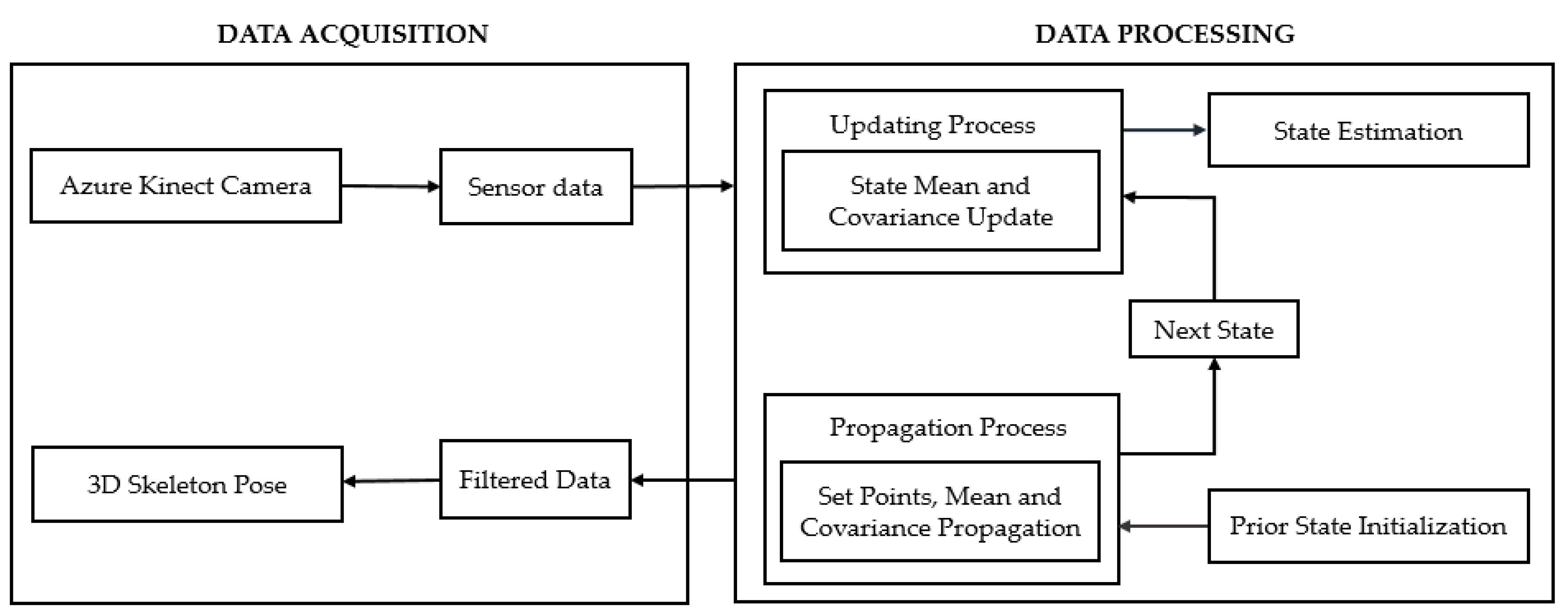
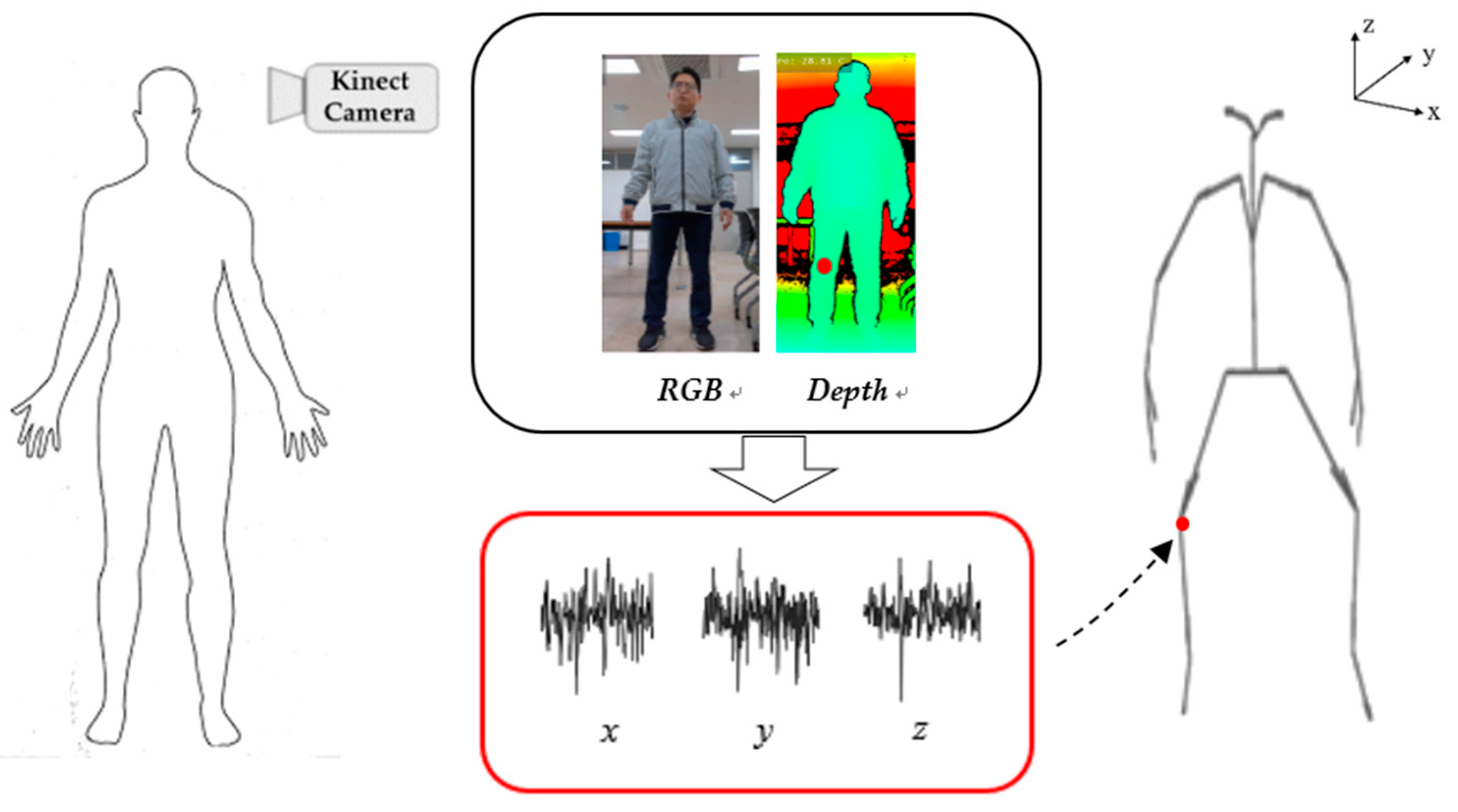
3. Proposed 3D Skeleton Posture Estimation Using a Randomized Unscented Kalman Filter

An EKF linearizes the nonlinear process model to estimate the state vector through Jacobian calculation. The EKF struggles to obtain the Jacobian estimate, which assumes nearly linear behavior for both the transition and observation function for more motion poses. This causes a significant difference in error while reconstructing the non-motion skeleton estimation and motion skeleton estimation. It is known that UKF is one of the methods for noise reduction while estimating a skeleton. It caused occasional instability in terms of state and measurement when reconstructing a skeleton estimation. To overcome these limitations, a novel noise reduction method based on an RUKF is proposed. The proposed method uses the data obtained from Microsoft Azure SDK. The concept of a skeleton is provided from the Kinect camera. The entire process, from the data acquisition to 3D skeleton estimation, through the filtering methods and expected simulated skeleton poses, is shown in Figure 2. These sensor data were modeled using conventional methods; as there is noise present in the data, to minimize, we proposed our method that includes key steps such as predict and update. The state transition function is used to predict the next state for the transition matrix, which is also called a state transition vector.

Let us consider the state transition function $f$, state $x$, and there is uncertainty $w$ (mean 0, and covariance Q), as follows:

$${{\displaystyle x}}_k=f\left(x_{k-1}\right)+w_k$$

(23)

The observation function $h$ used to obtain the transformations which use the rotation matrix to find the next joint obtained by the Euler angle and uncertainty $v$ (mean 0, and covariance R) along with the next joint state, as follows

$$z_k=h\left(x_k\right)+v_k$$

(24)

The procedure of RUKF consists of three steps: time update, prediction step, and measurement update. The proposed method is based on a stochastic integration rule (SIR) [35]. The SIR computed using the UT with spread and rotation N_max sigma point sets is random, which is represented as a randomized unscented transform (RUT) [36]. The purpose of this filter is to update the state covariance function at each time step (k). The initial parameters, i.e., k = 1, initial mean ${{\displaystyle \widehat{x}}}_0=0$, initial covariance P₀ = 0, maximum number of iteration steps N_max = 1, process noise covariance $Q_k$, predicted state ${\widehat{x}}_k^{-}$, and covariance $P_k^{-}$, can be expressed through the state transition function as follows:

$${\widehat{x}}_k^{-}=SIalg\left({\widehat{x}}_{k-1},P_{k-1},f\left(x\right),N_{max}\right)$$

(25)

$$P_k^{-}=SIalg\left({\widehat{x}}_{k-1},P_{k-1},f\left(x\right),N_{max}\right)+Q_k$$

(26)

The measurement estimate prediction can be obtained through the observation function h by the stochastic integration algorithm (SI alg) as

$${\widehat{z}}_k^{-}=SIalg\left({\widehat{x}}_k^{-},P_{{}_k}^{-},h\left(x\right),N_{max}\right)$$

(27)

The defined measurement covariance update function a(x), obtained through the observation function and measurement estimate prediction ${\widehat{z}}_k^{-}$ as

$$a\left(x\right)=\left(h\left(x\right)-{\widehat{z}}_{{}_k}^{-}\right){\left(h\left(x\right)-{\widehat{z}}_{{}_k}^{-}\right)}^T$$

(28)

The measurement covariance prediction $P_{{\widehat{z}}_k}{}_{{\widehat{z}}_k}$ can be obtained through covariance update function a(x), measurement-noise covariance $R_k$, and cross-covariance update function b(x); computed from the observation function h as follows:

$$P_{{\widehat{z}}_k}{}_{{\widehat{z}}_k}=SIalg\left({\widehat{x}}_{{}_k}^{-},P_{{}_k}^{-},a\left(x\right),N_{max}\right)+R_k$$

(29)

$$b\left(x\right)=\left(x-{\widehat{x}}_{{}_k}^{-}\right){\left(h\left(x\right)-{\widehat{z}}_{{}_k}^{-}\right)}^T$$

(30)

In the measurement update, cross-covariance $P_{x_k}{}_{z_k}$, can be obtained from sensor measurement, a cross-covariance update function b(x); and to combine all observation models, the Kalman gain $K_k$ contributes more or less weight to predict the observation as

$$P_{x_k}{}_{z_k}=SIalg\left({\widehat{x}}_{{}_k}^{-},P_{{}_k}^{-},b\left(x\right),N_{max}\right)$$

(31)

$$K_k=P_{x_k{z}_k}{P}_{{}_{{\widehat{z}}_k{\widehat{z}}_k}}^{-1}$$

(32)

All the updated state ${\widehat{x}}_k$ and covariance $P_k$ information from the state transition and observation models are combined as

$${\widehat{x}}_k={\widehat{x}}_k^{-}+K_k\left(z_k-{\widehat{z}}_k^{-}\right)$$

(33)

$$P_k=P_k^{-}-K_k{P}_{{\widehat{z}}_k{\widehat{z}}_k}{K}_k^T$$

(34)

At k = k + 1, the updated state covariance update $g\left(x\right)$ is expressed as

$$g\left(x\right)=\left(f\left(x\right)-{\widehat{x}}_{k-1}\right){\left(f\left(x\right)-{\widehat{x}}_{k-1}\right)}^T$$

(35)

Therefore, an RUKF is used to predict, update, and filter the kinematics motion for different skeleton poses. These skeleton poses are estimated by reducing the temporal noise for nonlinear estimation in state and observation transition models through the propagation and updating process iteratively. For each iteration, it will obtain the data from both the propagation and updating of RUKF. Moreover, it is possible to obtain the coordinates of each joint at computing state through the observation function. According to the authors of [30], the convergence of the system depends on an arbitrary function. We implemented the RUKF with an improved version of the SIR. Therefore, the arbitrary function is approximately constant, enabling the proposed algorithm to reach convergence. The pseudocode of Algorithm 3 is shown below.

Algorithm 3: Proposed method (RUKF)

Input: ${{\displaystyle z}}_k$ denotes the sensor-measured values of the k-frames. Output: ${{\displaystyle x}}_k$ denotes the estimated values of the k-frames. 1: Initial parameters k = 1, initial mean ${{\displaystyle \widehat{x}}}_0=0$, initial covariance ${{\displaystyle P}}_0=0$ 2: for k = 1 to N (maximum no. of iterations) do 3: State covariance update function: $g\left(x\right)$ (defined in the Equation (35)) Time update (prediction): 4: State prediction step: Predict ${\widehat{x}}_k^{-}$, and $P_k^{-}$ (defined in the Equations (25) and (26)) 5: Measurement estimate prediction ${\widehat{z}}_k^{-}$ using ${\widehat{x}}_k^{-}$, and $P_k^{-}$ (using step. 4) 6: Measurement covariance update function $a\left(x\right)$ using ${\widehat{z}}_k^{-}$ and an observation function $h\left(x\right)$(Using step. 5) 7: Measurement covariance update function $P_{{\widehat{z}}_k}{}_{{\widehat{z}}_k}$ (defined in the Equation (29)) using $a\left(x\right)$, ${\widehat{z}}_k^{-}$ and $P_k^{-}$ (Using the step. 6) 8: The cross-covariance update function $b\left(x\right)$ defined in the Equation (30) using ${\widehat{x}}_k^{-}$, $h\left(x\right)$ and ${\widehat{z}}_k^{-}$ Measurement update (correction) 9: Update the cross-covariance $P_{x_k}{}_{z_k}$ defined in Equation (31), Kalman gain $K_k$ defined in Equation (32), state estimate ${\widehat{x}}_k$ defined in Equation (33) and sate covariance $P_k$ (defined in Equation (34)) end for return estimated data (${{\displaystyle x}}_k$)

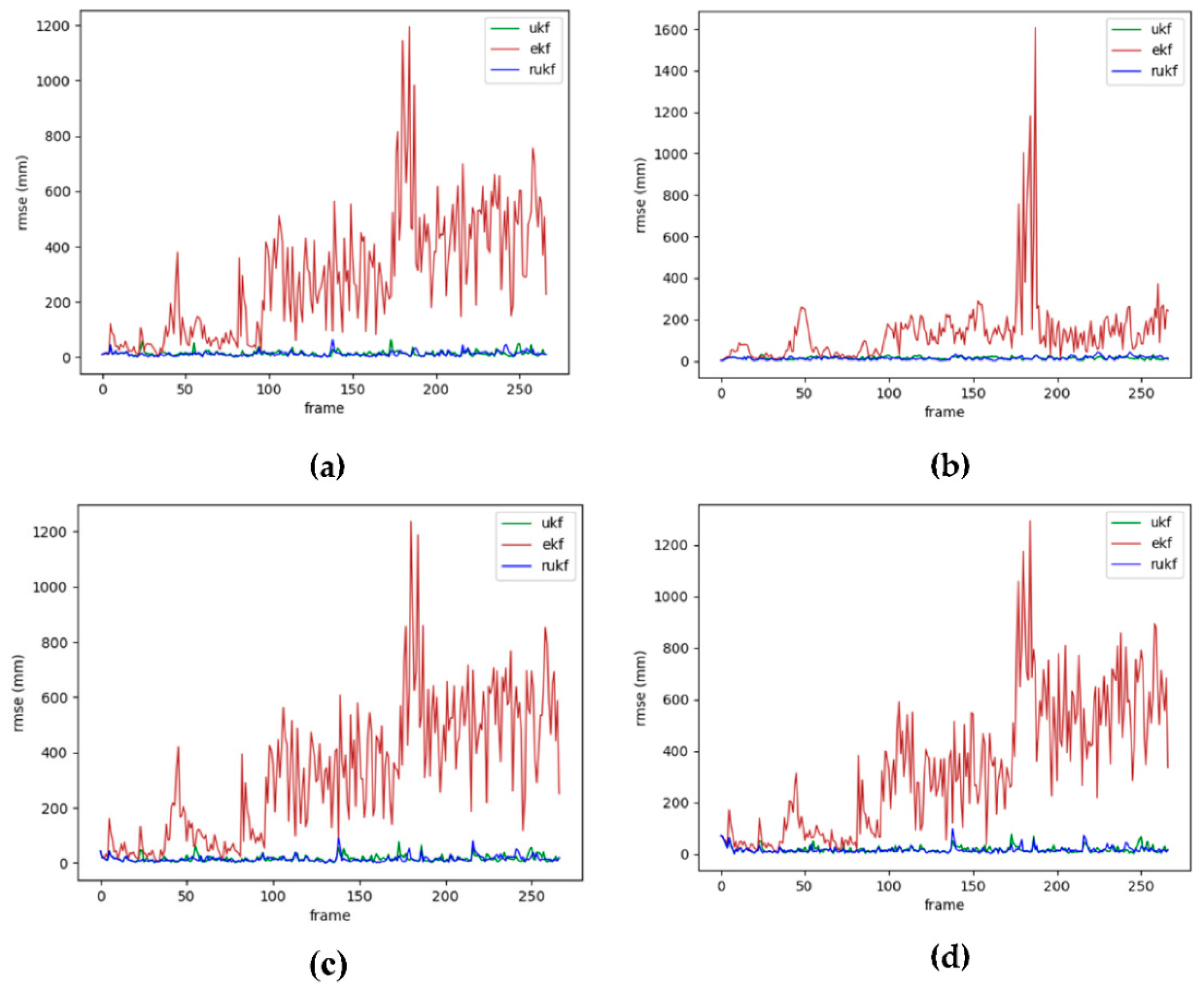
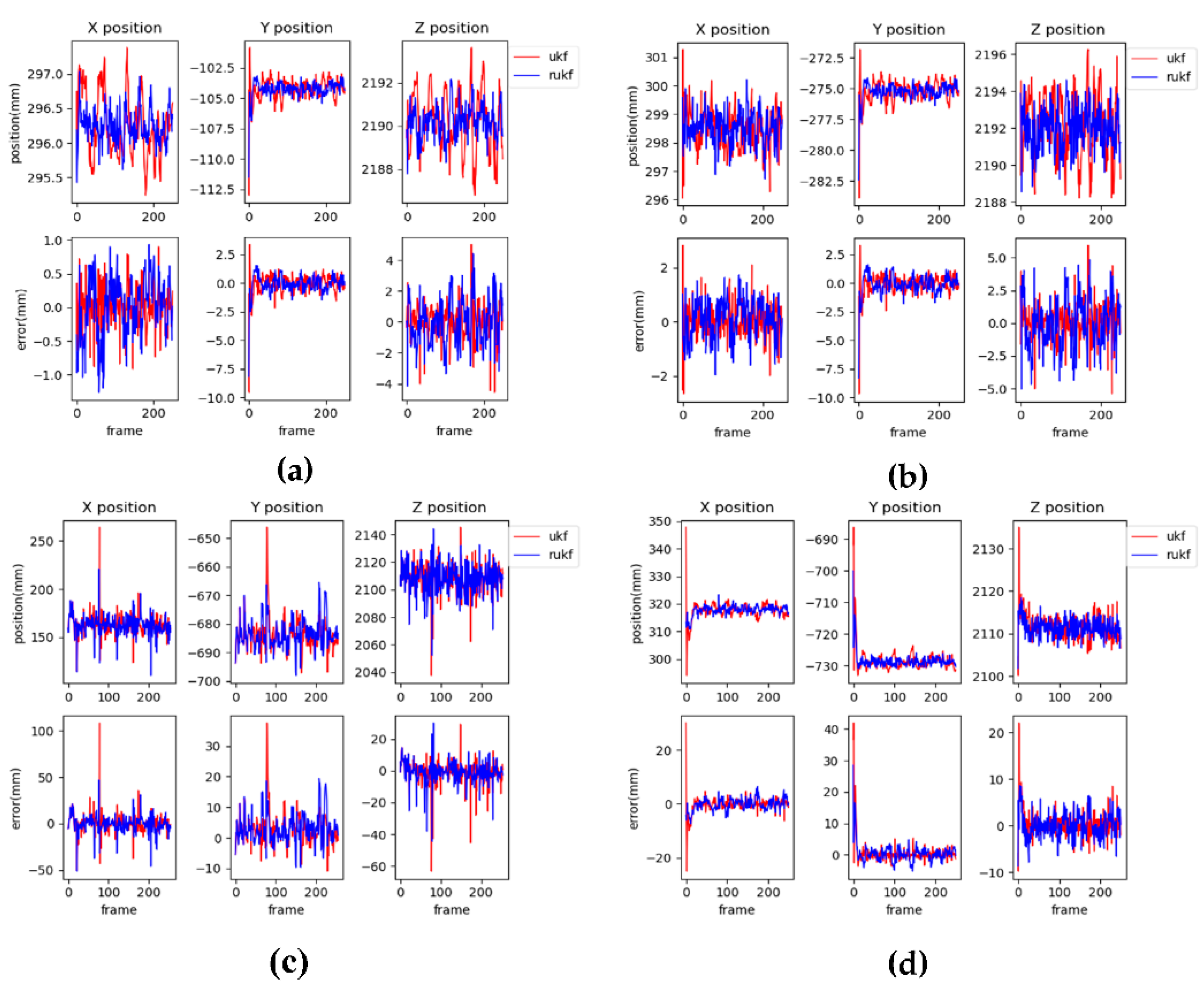
4. Experimental Results

The proposed method, tested with twelve poses, is considered as a manually annotated [37,38,39] dataset to evaluate its performance. It has been difficult to find standard public datasets for pose and skeleton estimation. Therefore, reference actions from [40,41] chose twelve poses, and the experiment was conducted with 20 participants to process the data. In this paper, the twelve pose datasets are as follows: Crossing arms, extending arms, flexion and extending, hands up, left standing, right standing, standing, unipedal, right flexion and extending, left flexion and extending, o–leg stand, and x–leg stand.

The tested dataset consists of 32 joints with the 30-s data, including the RGB and Depth information of each pose. The person would perform the pose in front of the Kinect camera to capture the pose. In the skeleton, each joint has its own joint coordinate system which is related to the depth camera 3D coordinate system. A skeleton includes 32 joints, with each connection linking the parent joint with a child joint. The pelvis is the root joint, fixed in the center of the human body followed by the child joints. For instance, the pelvis, which is the root joint, links to the spine_naval, which is the child joint; and the spine_navel (parent joint) links to the spine_chest (child joint). Euler angles and angular velocities are needed for the next child joint as the state, except for the root position, rather than using the 3D position coordinates of all skeletons. In each frame, the x, y, and z-coordinates of each joint are used to create a joint object instance for each of the 32 joints. Using the depth-first search algorithm, bone lengths are calculated and stored in the skeleton. To generate the skeleton map, the human body kinematic model splits into two: upper and lower body. In the calibration phase, the initial mean state vector of the lower body, and the initial mean state vector of the upper body, will be returned.

A model-filter controller function utilizes the lower and upper body properties to apply the proposed method. The Kinect data contained a number of frames, where the estimated data of the proposed method used every single frame. Subsequently, the estimated data were calculated with the help of filter objects, made in the previous step. The algorithm for one iteration was as follows. From the skeleton object list, the kth number of skeleton objects was selected, which was the skeleton for the kth frame. Then, the joint position of each joint of this frame was obtained, and the measurement vector ($z_k$) was calculated. Additionally, $z_k$ was used to calculate the updated state estimate for the kth frame. The updated mean and covariance are computed in the filter update method of the proposed method. From the updated state mean, the updated data for the current step are calculated by passing them through the observation function again. The updated mean and covariance are computed for lower and upper body models separately.

Finally, filter controller function retrieves and returns the covariance matrices for the upper and lower body using the proposed method. For comparison, we obtained the manually annotated ground truth [24,42,43,44,45,46] for the set of twelve poses captured by the camera. To analyze the original data and the estimated data, we employed the proposed method for determining the coordinates of each joint by incorporating the observation function at each iteration. The numerical comparison was conducted by incorporating the RMSE mean value (RMSE_mean) and the RMSE standard deviation value (RMSE_(±SD)) associated with the estimated data and ground truth, which were measured in millimeters (mm). The results show a comparison of the RMSE _mean and standard deviation (±SD) values in comparison with UKF, EKF and the proposed method. Examples of four joint points, i.e., pelvis, spine_naval, head and nose, are shown in Figure 3. In Figure 3a, the x-axis depicts the 30-s frame data, and the y-axis depicts the RMSE. There are rapid enhancements and large errors on the EKF.

The UKF and proposed method have similar results on Figure 3. Further, we will compare these with skeleton data on x, y, and z-coordinate systems. The joint variables and mean (±SD) of the RMSE values among the three nonlinear filters EKF, UKF, and proposed method are presented in

Table 1. Results of RMSE_mean and RMSE_(±SD) of skeleton joints for each method.

Joints	EKF		UKF		Proposed
	Mean	±SD	Mean	±SD	Mean	±SD
Pelvis	1.11	±0.46	0.58	±0.40	0.35	±0.26
Spine_Naval	1.78	±0.85	0.72	±0.60	0.28	±0.29
Spine_chest	1.31	±0.78	1.11	±0.81	0.39	±0.39
Shoulder_left	1.64	±0.72	1.41	±1.04	0.35	±0.19
Elbow_Left	1.77	±0.92	1.55	±1.80	0.49	±0.26
Hand_left	4.82	±3.04	4.78	±2.90	1.43	±0.86
Hand_Right	3.51	±1.80	3.18	±1.79	1.21	±0.77
Wrist_Left	4.23	±2.46	2.94	±1.91	1.37	±0.83
Eye_Right	3.42	±9.86	4.05	±9.68	1.58	±5.47
Ear_Right	5.83	±17.63	4.63	±15.6	1.60	±4.78

.

Joints of each pose are affected by the noise; the effected nonlinear temporal noise was filtered with nonlinear filters. Further, the EKF has the largest RMSE at the ear_right (5.83 ± 17.63) and the smallest RMSE at the pelvis (1.34 ± 0.57). Utilizing the UKF method, RMSE at the ear_right is (4.63 ± 15.6) and the value of the pelvis is (0.58 ± 0.40), the data demonstrate that there is a possibility to reduce the noise further. Finally, upon implementing the proposed method, the RMSE value for “ear_right” was found to be (1.60 ± 4.78), and the RMSE value for the pelvis was found to be (0.35 ± 0.26). Specifically, parts of the head including ‘eye_right’ and ‘ear_right’ moved more rapidly than the other joints of the body. This resulted in an increase in the SD compared to the other joints.

Finally, depending on the RMSE, the proposed method is proven to have superior performance across all the joints of the twelve poses. The estimated results of the x, y, z joint by UKF and the proposed method on the x, y, and z-coordinate systems are shown in Figure 4. This presents examples of four joint positions, i.e., pelvis, spine naval, head, and nose. Here, the x-axis is on a time domain, and the y-axis shows the position and its error. The error results of the UKF is indicated with the red line and the proposed method with the blue line. The error fluctuation by the proposed method is less than that by the UKF, as shown in Figure 4. This is because the proposed method compensates for the error, while using both the observation and state transition functions on a RUKF method. The performance of joint position connects to the skeleton estimation directly. The graphical results of skeleton estimate for twelve poses according to each algorithm are presented in Figure 5.

The skeleton estimation by the UKF and RUKF method is indicated as blue and green lines, respectively. These captured images are shown only single frame among 30-s in each pose. Therefore, there are some limitations to showing the experiments entirely. However, it is possible to evaluate the performance of the RUKF method using Table 1. The 3D skeleton map estimation by the proposed method has better results in terms of the quantitative results of RMSE_mean (±SD) than that of the UKF method in Figure 5.

5. Conclusions

This study proposed a method of 3D skeleton pose estimation using a randomized unscented Kalman filter to reduce nonlinear noises on a Kinect camera. The proposed method analyzed the propagation and updating process for temporal noises of skeleton data on the x, y, and z-coordinate systems. The accuracy of state estimation and prediction of the data are enhanced owing to the use of randomized UT. This enables the proposed method to correct errors that occur with the nonlinear temporal noise. Therefore, the experimental results show that the performance of the proposed method reduces the RMSE and SD while estimating the 3D skeleton map.

References

1. Sophie, A.; Sohaib, L.; Joelle, T.; Thierry, D. Action recognition based on 2D skeletons extracted from RGB videos. MATEC Web. Conf. 2019, 277, 1–14. [Google Scholar]
2. Aggarwal, J.K.; Xia, L. Human activity recognition from 3d data: A review. Pattern Recognit. Lett. 2014, 48, 70–80. [Google Scholar] [CrossRef]
3. Biswas, K.K.; Basu, S.K. Gesture recognition using Microsoft Kinect. In Proceedings of the 5th International Conference on Automation, Robotics and Applications, Wellington, New Zealand, 6–8 December 2011. [Google Scholar]
4. Xia, L.; Chia-Chih, C.; Aggarwal, J.K. Human Detection Using Depth Information by Kinect. In Proceedings of the Computer Vision and Pattern Recognition (CVPR), Colorado Springs, CO, USA, 20–25 June 2011. [Google Scholar]
5. Yunru, M.; Kumar, M.; Nichola, C.; Xiangbin, W.; Ye, M.; Yanxin, Z. The validity and reliability of a Kinect v2-based Gait Analysis system for children with cerebral Palsy. Sensors 2019, 19, 1–16. [Google Scholar]
6. Andersen, M.; Jensen, T.; Lisouski, P.; Mortensen, A.; Hansen, M. Kinect Depth Sensor Evaluation for Computer Vision Applications; Technical Report, ECE-TR-6; Department of Electrical and Computer Engineering, Aarhus University: Aarhus, Denmark, 2012; pp. 1–13. [Google Scholar]
7. Kong, L.; Xiaohui, Y.; Maharjan, A.M. A hybrid framework for automatic joint detection of human poses in depth frames. Pattern Recognit. 2018, 77, 216–225. [Google Scholar] [CrossRef]
8. Microsoft Azure Kinect Camera. Available online: https://www.microsoft.com/en-us/research/project/skeletal-tracking-on-azure-kinect (accessed on 10 April 2020).
9. Mallick, T.; Pratim Das, P.; Arun Kumar, M. Characterizations of Noise in Kinect Depth images: A review. IEEE Sens. J. 2014, 14, 1731–1740. [Google Scholar] [CrossRef]
10. Ju, S.; Sen-ching, S.C. Layer Depth Denoising and Completion for Structured-Light RGB-D Cameras. In Proceedings of the 2013 IEEE Conference on Computer Vision and Pattern Recognition, Portland, OR, USA, 23–28 June 2013. [Google Scholar]
11. Peter, F.; Michael, B.; Diego, R. Kinect v2 for Mobile Robot Navigation: Evaluation and Modeling. In Proceedings of the 2015 International Conference on Advanced Robotics (ICAR), Istanbul, Turkey, 27–31 July 2015. [Google Scholar]
12. Camplani, M.; Salgado, L. Efficient spatio-temporal hole filling strategy for Kinect depth maps. In Proceedings of the SPIE, Burlingame, CA, USA, 30 January 2012. [Google Scholar]
13. Nguyen, C.V.; Izadi, D.L.S. Modelling Kinect sensor noise for improved 3D reconstruction and tracking. In Proceedings of the 2012 Second International Conference on 3D Imaging, Modeling, Processing, Visualization & Transmission, Zurich, Switzerland, 13–15 October 2012. [Google Scholar]
14. Lin, B.; Su, M.; Cheng, P.; Tseng, P.; Chen, S. Temporal and spatial denoising of depth maps. Sensors 2015, 15, 18506–18525. [Google Scholar] [CrossRef] [PubMed] [Green Version]
15. Costilla-Reyes, O.; Scully, P.; Ozanyan, K.B. Temporal pattern recognition in gait activities recorded with a footprint imaging sensor system. IEEE Sens. J. 2016, 16, 8815–8822. [Google Scholar] [CrossRef]
16. Essmaeel, K.; Gallo, L.; Damiani, E.; De Pietro, G.; Albert Dipanda, A. Temporal denoising of Kinect depth data. In Proceedings of the 2012 Eighth International Conference on Signal Image Technology and Internet Based Systems, Naples, Italy, 25–29 November 2012. [Google Scholar]
17. Sergey, M.; Vatolin, D.; Yury, B.; Maxim, S. Temporal filtering for depth maps generated by Kinect depth camera. In Proceedings of the 2011 3DTV Conference: The True Vision—Capture, Transmission and Display of 3D Video (3DTV-CON), Antalya, Turkey, 16–18 May 2011. [Google Scholar]
18. Simone, M.; Giancarlo, C. Joint denoising and interpolation of depth maps for MS Kinect Sensors. In Proceedings of the 2012 IEEE International Conference on Acoustics, Speech and Signal Processing (ICASSP), Kyoto, Japan, 25–30 March 2012. [Google Scholar]
19. Rashi, C.; Dasgupta, H. An approach for noise removal on Depth Images. In Proceedings of the Computer Vision and Pattern Recognition, Las Vegas, NV, USA, 27–30 June 2016. [Google Scholar]
20. Junyi, L.; Xiaojin, G.; Jilin, L. Guided In painting and filtering for Kinect Depth Maps. In Proceedings of the 21st International Conference on Pattern Recognition (ICPR 2012), Tsukuba, Japan, 11–15 November 2012. [Google Scholar]
21. Loumponias, K.; Vretos, N.; Daras, P.; Tsaklidis, G. Using Kalman filter and Tobit Kalman filter in order to improve the motion recorded by Kinect sensor II. In Proceedings of the 29th Panhellenic statistics conference, Nassau, Bahamas, 4–7 May 2016. [Google Scholar]
22. Del Rincón, J.M.; Makris, D.; Uruñuela, C.O.; Nebel, J.C. Tracking human position and lower body parts using Kalman and particle filters constrained by human biomechanics. IEEE Trans. Syst. Man Cybern. Part B 2011, 41, 26–37. [Google Scholar] [CrossRef]
23. Jody, S.; Fumio, H.; John, A. Application of extended Kalman filter for improving the accuracy and smoothness of Kinect skeleton-joint estimates. J. Eng. Math. 2014, 88, 161–175. [Google Scholar]
24. Amir, B.; Lora, C.; John, L.C. Hip and Trunk kinematics estimation in gait through Kalman filter using IMU data at the Ankle. IEEE Sens. J. 2018, 18, 4253–4260. [Google Scholar]
25. Gustafsson, F.; Hendeby, G. Some relations between extended and unscented Kalman filters. IEEE Trans. Signal Process. 2012, 60, 545–555. [Google Scholar] [CrossRef] [Green Version]
26. Manuel, G. Kinematic Data Filtering with Unscented Kalman Filter-Application to Senior Fitness Tests Using the Kinect Sensor; University of Lisbon: Lisbon, Portugal, 2017; pp. 1–8. Available online: https://fenix.tecnico.ulisboa.pt (accessed on 1 March 2020).
27. Moon, S.; Park, Y.; Ko, D.W.; Suh, H. Multiple Kinect Sensor Fusion for Human Skeleton Tracking Using Kalman Filtering. Int. J. Adv. Robot. Syst. 2016, 13, 1–10. [Google Scholar] [CrossRef] [Green Version]
28. Julier, S.J.; Uhlmann, J.K. A new extension of the Kalman filter to nonlinear systems. In Proceedings of the Signal Processing, Sensor Fusion, and Target Recognition VI, Orlando, FL, USA, 21–25 April 1997. [Google Scholar]
29. Carpenter, J.; Clifford, P.; Fearnhead, P. An improved particle filter for non-linear problems. IEEE Proc. Radar Sonar Navig. 1999, 146, 2–7. [Google Scholar] [CrossRef]
30. Li, T.; Bolic, M.; Djuric, P.M. Resampling methods for particle filtering: Classification, implementation, and strategies. IEEE Signal Process. Mag. 2015, 32, 70–86. [Google Scholar] [CrossRef]
31. Elfring, J.; Torta, E.; van de Molengraft, R. Particle Filters: A Hands-On Tutorial. Sensors 2021, 21, 438. [Google Scholar] [CrossRef] [PubMed]
32. Gustafsson, F.; Gunnarsson, F.; Bergman, N.; Forssell, U.; Jansson, J.; Karlsson, R.; Nordlund, P.J. Particle Filters for Positioning, Navigation, and Tracking. IEEE Trans. Signal Process. 2002, 50, 425–437. [Google Scholar] [CrossRef] [Green Version]
33. Nobahari, H.; Zandavi, S.M.; Mohammadkarimi, H. Simplex filter: A novel heuristic filter for nonlinear systems state estimation. Appl. Soft Comput. 2016, 49, 474–484. [Google Scholar] [CrossRef]
34. Zandavi, S.M.; Vera, C. State estimation of nonlinear dynamic system using novel heuristic filter based on genetic algorithm. Soft Comput. 2018, 23, 5559–5570. [Google Scholar] [CrossRef]
35. Straka, O.; Dunik, J.; Simandl, M. Randomized Unscented Kalman Filter in Target Tracking. In Proceedings of the 2012 15th International Conference on Information Fusion, Singapore, 9–12 July 2012. [Google Scholar]
36. Dunik, J.; Straka, O.; Simandl, M. The development of a Randomized Unscented Kalman Filter. IFAC Proc. Vol. 2011, 44, 8–13. [Google Scholar] [CrossRef] [Green Version]
37. Fei, H.; Brian, R.; William, H.; Hao, Z. Space time representation of people based on 3D skeletal data: A review. Comput. Vis. Image Underst. 2017, 158, 85–105. [Google Scholar]
38. Tenorth, M.; Bandouch, J.; Beetz, M. The TUM kitchen data set of everyday manipulation activities for motion tracking and action recognition. In Proceedings of the IEEE 12th International Conference on Computer Vision workshops, Kyoto, Japan, 27 September–4 October 2009. [Google Scholar]
39. Kazemi, V.; Burenius, M.; Azizpour, H.; Sullivan, J. Multi-view body part recognition with random forests. In Proceedings of the British Machine Vision Conference, Bristol, UK, 9–13 September 2013. [Google Scholar]
40. Alexandre, B.; Christian, V.; Sergi Bermudez, B.; Élvio, G.; Fátima, B.; Filomena, C.; Simão, O.; Hugo, G. A dataset for the automatic assessment of functional senior fitness tests using Kinect and physiological sensors. In Proceedings of the International Conference on Technology and Innovation in Sports, Health and Wellbeing (TISHW), Vila Real, Portugal, 1–3 December 2016. [Google Scholar]
41. Liu, J.; Shahroudy, A.; Perez, M.; Wang, G.; Duan, L.; Kot, A.C. NTU RGB+D 120: A Large-Scale Benchmark for 3D Human Activity Understanding. IEEE Trans. Pattern Anal. Mach. Intell. 2020, 42, 2684–2701. [Google Scholar]
42. Marco, C.; Matteo, M.; Emanuele, M. Skeleton estimation and tracking by means of depth data fusion from depth camera networks. Robot. Auton. Syst. 2018, 110, 151–159. [Google Scholar]
43. George, R.; Kyria, P.; Anita, B. A method for determination of upper extremity kinematics. Gait Posture 2002, 15, 113–119. [Google Scholar]
44. Ben, C.; Adeline, P.; Sion, H.; Majid, M. Skeleton-Free Body Pose Estimation from Depth Images for Movement Analysis. In Proceedings of the 2015 IEEE International Conference on Computer Vision Workshop (ICCVW), Santiago, Chile, 7–13 December 2015. [Google Scholar]
45. Wei, S.; Ke, D.; Xiang, B.; Tommer, L. Exemplar-Based Human Action Pose Correction and Tagging. In Proceedings of the 2012 IEEE Conference on Computer Vision and Pattern Recognition, Providence, RI, USA, 16–21 June 2012. [Google Scholar]
46. Adeline, P.; Lili, T.; Sion, H.; Massimo, C.; Dima, D.; Majid, M. Online quality assessment of human movement from skeleton data. In Proceedings of the British Machine Vision Conference 2014, Nottingham, UK, 1–5 September 2014. [Google Scholar]
Figure 1. Flowchart of a sensor system based on the RUKF.
Electronics 10 00971 g001
Figure 2. Concept of skeleton joints composed using the RGB + D camera for the 3D skeleton estimation.
Electronics 10 00971 g002
Figure 3. Comparison of the RMSE results of EKF, UKF, and proposed method; (a) Pelvis, (b) Spine_ navel, (c) Head, and (d) Nose.
Electronics 10 00971 g003
Figure 4. Comparison of the position error of joints with the UKF, and proposed method; (a) Pelvis, (b) Spine_navel, (c) Head, and (d) Nose.
Electronics 10 00971 g004
Figure 5. Results of 3D skeleton estimation using UKF and the proposed method.
Electronics 10 00971 g005