Backup Capacity Planning Considering Short-Term Variability of Renewable Energy Resources in a Power System

Abstract

Increasing renewable energy penetration rate in a power grid leads to an increase in the variability of the generated energy, which increases the system integration cost. To handle the output variations in the generation, it is necessary to secure sufficient flexible resources, such as energy storage units. Flexible resources can adjust the output quickly, which helps to increase the system flexibility. However, the electricity generation cost of the flexible resources is usually high. Because the renewable energy expansion policy is being implemented worldwide, it is necessary to evaluate the ability to manage the short-term variations of the renewable energy outputs to obtain a cost-effective long-term plan. In this study, the variability of renewable energy in Korea over the past five years was analyzed. Additionally, the backup capacity is determined to manage the variability of renewable energy output. The backup capacity is affected by system flexibility. In general, increasing system flexibility decreases the backup capacity and increases the total electricity production cost. In this study, a backup capacity planning method is proposed considering the short-term variability of renewable energy output and flexibility deficit in a power system. The numerical results illustrated the effectiveness of the proposed backup capacity planning method.

1. Introduction

With the signing of the Paris Climate Agreement in 2015 and the inauguration of a new climate system, changes are taking place throughout the global power industry [1]. To achieve the goal of reducing carbon emissions, countries around the world are making various efforts, such as implementing a certified emission reduction (CER) system, expanding the proportion of renewable energy, expanding the supply of eco-friendly electric vehicles, and improving energy efficiency. In accordance with this global trend, the Korean government announced the 3020 Renewable Energy Plan, which will increase the share of renewable energy generation to 20% by 2030 [2,3]. However, this policy for increasing the penetration rate of renewable energy resources can cause problems that result in an increase in system costs [4,5]. The Nuclear Energy Agency (NEA) under the Organization for Economic Cooperation and Development (OECD) calculated the related costs by classifying them as the backup cost to respond to renewable energy variability, balancing cost to respond to the uncertainty of prediction, and grid cost to access power system [4]. Ku Leuven classified the system costs as backup (or profile) cost, balancing cost, and grid cost [5]. Additional studies were conducted on the costs related to expanding renewable energy [6,7,8]. This study was focused on the backup cost to evaluate the variability among other costs of employing renewable energy resources.

The output of renewable energy resources varies depending on the weather conditions. However, weather conditions are difficult to predict because they can change rapidly at any time. The forecast of renewable energy output is unreliable because of uncertain weather forecasts. This variability of renewable energy makes it difficult to balance supply and demand [9]. Many studies have been conducted on the variability of renewable energy [10,11,12]. Related to system flexibility, the variability of renewable energy means the variation in the output of renewable generation units owing to the rapid changes in weather conditions. In addition, the flexibility of the power system means the ability to maintain the balance between power supply and demand and maintain operating reserve requirements at all times in response to the variability within the power system [13,14]. The lack of system flexibility may lead the power system to fail in responding to rapid demand changes and collapse.

Reliable system operation requires sufficient flexibility and reserve in the system. Without enough flexible generation resources, new generation resources are needed to provide additional system flexibility. The amount of generation resources required for this new construction is defined as the backup capacity (BC). In general, these flexible resources include energy storage systems (ESSs) and gas turbines with short startup hours (SUH) and high ramp rates (RR) [15]. However, these generation resources have a higher production cost compared to inflexible generation resources, such as nuclear and coal power plants. Investment in these flexible generation resources increases the reliability of the power system, while it requires a higher level of investment. Hence, the economics of backup generation expansion needs to be evaluated from a power system planner’s point of view [16]. Overinvestment in new facilities increases the pertaining costs. Conversely, if a new facility is underinvested, it cannot cope with sudden fluctuations in production and may cause power outages, which incur excessive costs [17].

Therefore, the appropriate investment of BC needs to be analyzed by minimizing integrated backup operating cost and backup investment cost. This paper presents a systematic method for power system planners to perform an appropriate level of backup capacity planning. In assessing power system flexibility, time horizons are separated, and corresponding flexibility resources are selected for each time horizon. The proposed method is designed to minimize the combined backup operating and investment costs while maintaining an appropriate level of power system reliability.

Several studies have been conducted to evaluate the flexibility of the power system in various time horizons [15,18,19,20,21,22]. Andrew Mills et al. analyzed flexibility supply in various time horizons (15 min, 1 h, 6 h, 36 h) by measuring the capacity of generation or demand to change in response to system conditions. In addition, flexible demand was analyzed through the amount of net demand expected to change at each time period [15]. Thomas et al. evaluated the annual, weekly, and daily flexibility requirements of the French power system through frequency spectrum analysis and performed a sensitivity analysis by setting five variables: network interconnection, penetration of wind power, solar power, electric heating, and electric cooling [18]. Akylas C. Stratigakos et al. evaluated flexibility in the Greek power system over the time horizons, as shown in [15]. The number of flexibility needs and flexibility resources were determined for 15 min, 1 h, 6 h, and 36 h, and the flexibility of the Greek system was evaluated through the flexibility index (FIX) [19]. Most of the existing studies have analyzed the flexibility by dividing the time horizons, but considering the short-term ramping characteristics of ESS or GTs, it is necessary to analyze it by dividing it into more detailed time horizons. Flexibility evaluation without detailed classification for the short-term may have insufficient flexibility for rapid changes in a certain period and may result in an inadequate BC.

Variable renewable energy (VRE) stands for renewable energy resources with high output fluctuations, such as solar and wind power. Most existing studies considered only the effects of one of the remaining resources, using methods such as fixing the output of either resource [23,24,25]. To perform an accurate simulation, this study examined the trend of output variation that occurred when the output of these two resources was combined [26,27,28,29,30]. Based on this scenario, a serious situation was assumed because long-term plans require sufficient resources to cope with the worst situation [15,19]. Assuming severe conditions, a new approach is introduced to calculate the BC.

As the penetration rate of renewable energy resources increases, variability within a short period is expected to increase rapidly. Therefore, a long-term facility plan should be carried out considering the short-term variability of renewable energy. If the VRE increases, the system operator needs to reduce the output of flexible generators to maintain a balanced supply and demand. This reduction in generators’ output is related to the downward system flexibility and can be resolved by limiting renewable energy output if the system is unable to cope with upward fluctuations [15,20]. Conversely, the downward movement of renewable energy requires an increase in the output of flexible generators, which in turn requires secure flexible resources. This study was focused on the amount of upper secured, flexible resources. Therefore, the downward output variation of renewable energy was analyzed.

A method is introduced for evaluating flexibility in long-term facility planning and calculating optimal BC considering short-term variability of renewable energy, generator characteristics, and construction cost of backup facilities. In addition, the calculation of the optimal BC of the Korean power system in 2030 is provided. Furthermore, the abbreviations of this paper are represented in Abbreviations.

2. Power System Flexibility and Variability of Renewable Energy

2.1. Flexibility of Power System

In long-term planning, it is necessary to analyze whether sufficient system flexibility resources are secured to cope with the variability of renewable energy considering the generator ramp rate. Resources that can provide flexibility to cope with short-term fluctuations can be classified according to the time horizons as shown in

Table 1. Flexible resources according to the time horizons.

Status	Within 5 min	30 min	60 min	120 min
Online	Remaining Capacity of Online Flexible Power Plants
Offline	Battery energy storage, pumped-hydro Energy storage, etc.	Gas turbine (SUH * < 30 min), Pumped-hydro Energy storage, etc.	Gas turbine (SUH < 60 min), Pumped-hydro Energy storage, etc.	Combined cycle GT (SUH < 120 min), etc.

* Startup Hour.

.

System flexibility (SF) is calculated by summing the amount of flexibility provided by the online and offline generators [20].

$$S{F}_t = Fle{x}_{ON,t} + Fle{x}_{OFF,t}$$

(1)

where t represents the time horizon. The flexibility available for online generators $Fle{x}_{ON,t}$ can be calculated as follows:

$$Fle{x}_{ON,t}={\displaystyle \sum }_{n\in ON }Min\left[R{R}_n\times t,\hspace{1em}{P}_{max,n}-P_{BP,n}\right]$$

(2)

where $R{R}_n$ represents the ramp rate of generator n, $P_{max,n}$ represents the maximum output capacity of generator n, and $P_{BP,n}$ is the base point of the generator n, that is, the operating point.

System flexibility is determined by the operating level of the flexible generators. If the generator has a high operating point for the rated capacity, the spare capacity that the generator can additionally supply becomes less, which reduces system flexibility. On the contrary, when the generator has a low operating point, the capacity that can be additionally supplied increases, and thus the system flexibility increases. As nuclear and coal power plants are inflexible resources, the most flexible resources are combined cycle gas turbines (CCGTs).

The flexibility available for the offline generator $Fle{x}_{OFF,t}$ can be calculated as follows:

where SUH represents the generator startup hour, which means the time required for the generator to move from offline to online mode.

$$Fle{x}_{OFF,t}={\displaystyle \sum }_{m\in OFF }Min\left[R{R}_m\times \max \left(t-SU{H}_m,0\right),\hspace{1em}{P}_{max,m}\right]$$

(3)

2.2. Variability of Renewable Energy

To determine whether the aforementioned power system flexibility is sufficient, its ability to cope with the fluctuations of renewable energy is checked. The variability of renewable energy tends to appear differently according to each time horizon and the capacity factor of renewable energy. The proposed method of calculating the variability is introduced and analyzed at each time horizon using the output of variable renewable energy (VRE). Additionally, the relationship between the capacity factor and variability of renewable energy is analyzed because the level of the variability varies depending on the capacity factor, which may vary to some extent in different countries and power system topologies. Only downward variability of VRE was studied, where the output was decreasing.

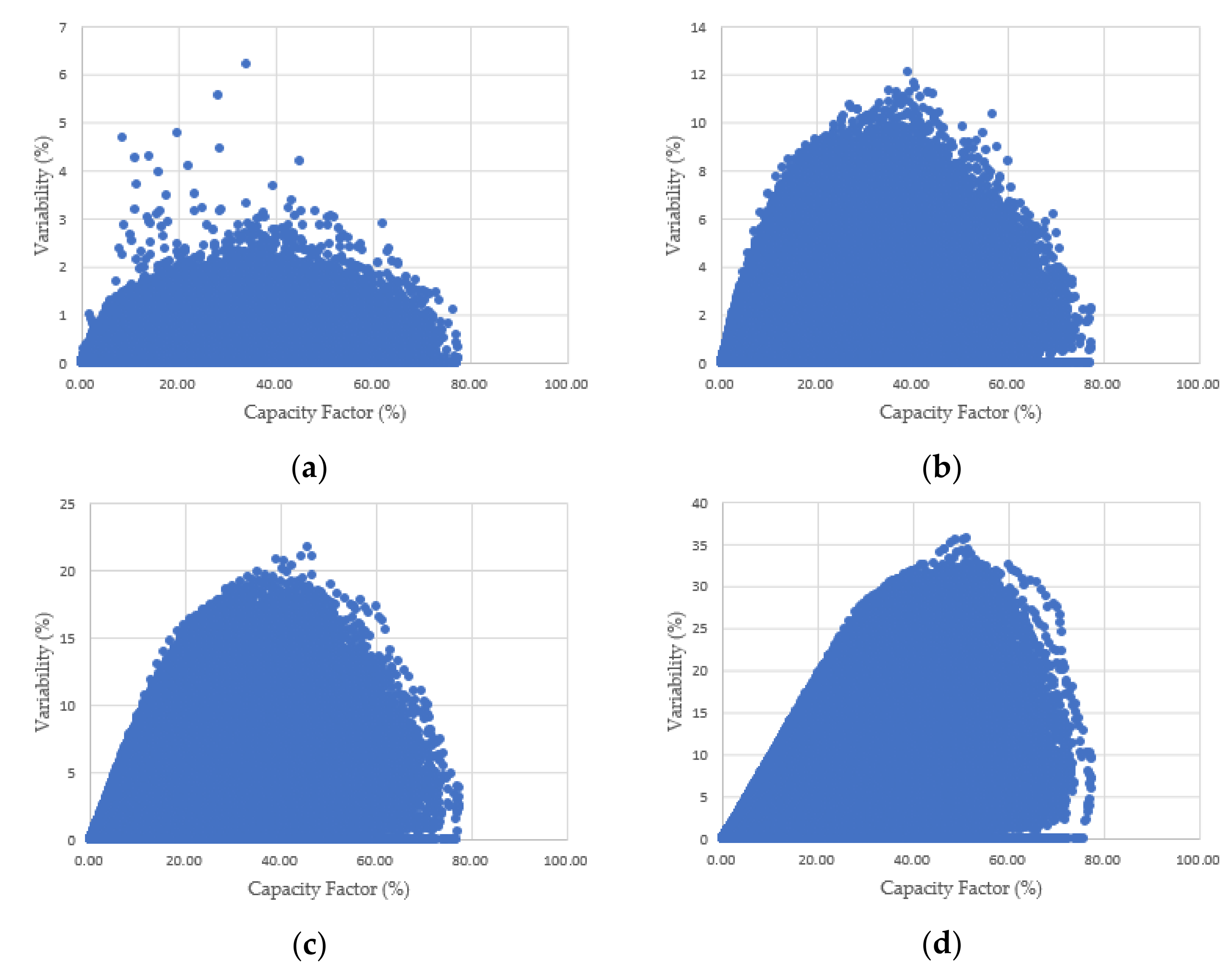
2.2.1. Variability at Each Time Horizon

Variability of VRE was calculated considering the simultaneous output of solar and wind power units in different time horizons as well as their capacity and variability, which were reflected in the test power system. The variability at a specific point in time t is as follows:

$$Va{r}_{VRE,t,t+5} = \frac{Ge{n}_{VRE,t} - Ge{n}_{VRE,t+5} }{Ca{p}_{VRE,t }} \times 100\left(\%\right)$$

(4)

where $Ge{n}_{VRE,t }$ and $Ge{n}_{VRE,t+5}$ represent the VRE output (MW) at the time t (min) and t +5 min, respectively. Further,$Ca{p}_{VRE,t}$ is the VRE facility capacity (MW) at the time t (min), which is the sum of the capacity of solar and wind at the time t.

In this study, classification of the variability of 30, 60, and 120 min time horizons was carried out and is described in

Table 2. Variability at each time horizon.

Time Horizon	Value
5 min	$Va{r}_{VRE,t,t+5}$
30 min	$Max\left(Va{r}_{VRE,t,t+5}, Va{r}_{VRE,t,t+10}, Va{r}_{VRE,t,t+15}, \cdots , Va{r}_{VRE,t,t+30}\right)$
60 min	$Max\left(Va{r}_{VRE,t,t+5}, Va{r}_{VRE,t,t+10}, Va{r}_{VRE,t,t+15}, \cdots , Va{r}_{VRE,t,t+60}\right)$
120 min	$Max\left(Va{r}_{VRE,t,t+5}, Va{r}_{VRE,t,t+10}, Va{r}_{VRE,t,t+15}, \cdots , Va{r}_{VRE,t,t+120}\right)$

. The reason behind this was that the flexibility of each time horizon could be evaluated by applying the constraints of power generation resources at each time horizon to respond to the variability.

For example, the 30 min variability at the time t is the largest among the variability after 5, 10, 15, 20, 25, and 30 min from the analysis time point t. It is important to select an appropriate level of variability according to the study goals. To cope with the variability of VRE with a maximum of 99.73 percentiles (+3 sigma), average variability or other criteria can be applied. Since this study aimed to measure the flexibility to cope with the largest variability of VRE from the perspective of long-term planning, the maximum variability for each time horizon was applied. The analysis was based on the data collected over the last five years (2014–2018) from renewable energy outputs in the Korean Power System.

2.2.2. Variability According to the Output of Renewable Energy Resources

Figure 1 shows the performance of VRE and trends of the variability change depending on the level of a capacity factor in Korea over the past five years (2014–2018).

In each 5 min time interval, variability is evenly distributed in terms of the capacity factor compared to other time horizons. In the frames of 60 and 120 min, the variability in terms of the capacity factor follows the form of the y ≤ x graph because the output of VRE cannot change more than the output itself. In the frame of 120 min, it can be seen that a large variability occurs at a relatively high capacity factor. Therefore, the effect of sunset has appeared since the variability is downward.

VRE has a high or maximum level of variability in the capacity factor of 30 to 60%. The maximum variability does not occur at the maximum capacity factor, where the variability is generally smaller than that of the intermediate level.

When the capacity factor of VRE is divided into three sections by 30%, the maximum variability within the sections is shown in

Table 3. The maximum variability of renewable energy within the sections of capacity factor.

Time Horizon	Low Level (0–30%)	Mid Level (30–60%)	High Level (60–100%)
5 min	5.57	6.21	2.92
30 min	10.77	12.08	7.29
60 min	18.80	21.77	16.53
120 min	27.94	35.81	32.08

. The larger the time horizon, the greater the variability of the VRE is selected over a wide range of time. This trend is the same at the maximum and 99.73 percentiles.

The values of maximum variability within the sections of the capacity factor are shown in Table 3. The maximum level of variability in all time horizons is the highest at 30–60% of the capacity factor.

3. Flexibility Deficit and Optimal Backup Capacity

A definition of the flexibility deficit (FD) and a method for determining the BC required in long-term plans is presented in this section to cope with the short-term variability of renewable energy analyzed in Section 2. FD is a deficient amount to cope with the variability of renewable energy resources and varies with the system flexibility. To calculate the optimal backup capacity (OBC) to cope with the FD, an economical plan of the BC construction is needed.

3.1. Flexibility Deficit

Long-term planning should assume the most severe conditions of the year and analyze whether sufficient resources are available to respond to them. In general, lower demand results in a less flexible system. This is because the share of inflexible power sources, such as nuclear power plants in generation systems, increases. On the other hand, the variability of renewable energy tends to be different depending on the output level of renewable energy, as analyzed in Section 2.2. Therefore, to find the most severe conditions, scenarios should be classified according to the load level and renewable energy output level.

To calculate the FD according to the set scenarios, some assumptions were made. It was assumed that nuclear and coal power plants, which are inflexible power generation sources, produce constant output considering the forced outage rate (FOR) and maintenance outage rate (MOR). FOR and MOR, respectively, is the probability to be unable to produce power due to unexpected breakdown and maintenance. The bigger FOR and MOR are considered in the long-term planning, the more facility investment is required to ensure the system’s reliability. Moreover, the output of renewable energy resources, nuclear power plants, and coal generators was deducted from the demand consecutively, and combined cycle gas turbine (CCGT) took over the remaining demand. As for CCGT, a representative generator was set. This representative generator was added one-by-one subsequently at the same operating point until the supply met the demanding output. Moreover, the last added generator took over the remaining demand. At this time, if the minimum power generation constraint is violated, all online CCGTs should take over the remaining demand equally. If supply exceeds demand, the output of renewables is curtailed. As the operating point of the CCGTs decreased, the spare capacity per unit and the number of online units increased, thereby increasing the flexibility of the system. Consequently, according to the operating point of the CCGT, the FD is calculated as follows:

$$F{D}_{t,op}^{sc}=Re{s}_t+Va{r}_{VRE,t}-S{F}_{t,op}^{sc} \left(t=5, 30, 60, 120 min\right)$$

(5)

where t represents the time horizon, op represents the operating point of the CCGT, and sc represents the scenario. For instance, $F{D}_{30,0.8}^{s1}$ represents FD in the 30 min time interval of scenario 1 at the combined cycle 0.8 operating point. $Re{s}_t$ is the reserve required by the electricity market regulator, $Va{r}_{VRE,t}$ is the maximum variation of VRE, and $S{F}_t$ is the system flexibility.

In this study, $F{D}_{t,op}$ was calculated as the maximum value among the $F{D}_{t,op}^{sc}$ of all the scenarios in the period as follows:

$$F{D}_{t,op}=MAX\left(F{D}_{t,op}^{sc},0\right)$$

(6)

If $F{D}_{t,op}$ is greater than zero, the system lacks flexibility, and an additional backup facility is required. If it is less than zero, the system flexibility is sufficient, and no additional backup facility is required.

3.2. Optimal Backup Capacity

The FD is calculated in terms of the operating point, as described in Section 3.1. A decrease in the operating point of the CCGT increases the system flexibility and decreases the BC. Therefore, the backup construction cost from increasing BC is proportional to the operating point of the CCGT. However, as the operating point of CCGT decreases, the efficiency of the generator decreases, and the generator with a higher cost of power generation operates, increasing the annual electricity production cost. Conversely, as the operating point increases, the annual electricity production cost decreases. Thus, it is necessary to determine the optimal operating point of the CCGT considering not only BC construction cost but also electricity production cost.

Therefore, the simulation should be repeated while changing the basepoint (operating point) of the CCGT. The operating point, at which the sum of the construction cost for the BC and the electricity production cost is minimum, the optimal operating point of the CCGT in the long-term is achieved. The BC, at this point, gains the optimal value.

As this study dealt with long-term planning, the annual electricity production cost was calculated using the priority list method unit commitment, which is mainly used in long-term planning. In long-term planning, performing detailed unit commitment (UC) and economic dispatch (ED) makes electricity production cost calculations time-consuming; therefore, simple modeling and simulation should be utilized. In this study, nuclear and coal power plants were output at a constant annual rate considering the forced outage rate. Accordingly, the electricity production costs of nuclear and coal power plants are constant. For the remaining load, after subtracting the output of nuclear power (fixed), coal (fixed), and renewables (various) from the 1 h load, the CCGT generator becomes operational to balance supply and demand, where cheaper generators go online earlier.

Our study converted the backup construction costs into annual backup construction costs by applying the equated annual installment using Equation (7):

$$Annual Backup Construction Cost = \frac{P\times {\left(1+r\right)}^n\times r}{{\left(1+r\right)}^n-1}$$

(7)

In Equation (7), P is the backup facility construction cost, n is the economic life of the facility, and r is the discount rate.

The minimum point by summing the annual construction cost and result of annual electricity production cost in terms of the operating point of the CCGT is the optimal CCGT operating point, and the BC at this point takes the optimal value. Figure 2 shows the optimal CCGT operating point and BC.

3.3. The BC Planning Considering Short-Term Variability of Renewable Energy Resources

The process consists of the following five steps: (1) receiving data, (2) predicting renewable sources output and forecasting the hourly load, (3) finding the BC construction cost using the operating points, (3) finding electricity production cost using the operating points, (4) calculating the optimal operating point, and (5) determining the optimal BC.

To present each step in detail, First, the system planners must acquire basic data, such as the variability, load pattern, and generator characteristics, using historical data. These basic data can be obtained through supervisory control and data acquisition (SCADA). In addition, projected data, such as renewable energy output based on past patterns, projected generator facilities, and future 5 min demand based on past demand patterns, should be created. Such projected data may vary according to the criteria targeted by national policies. Next, the flexibility deficit (FD) and backup capacity (BC) in terms of the operating points in a severe condition are calculated. When calculating FD, consider whether there is sufficient system flexibility as the sum of the reserve criteria and the maximum amount of renewable energy variability. If FD occurs, calculate BC for each time horizon, considering the startup hour and ramp rate of flexible resources. On the, while, using priority list method unit commitment (PLUC), the electricity production cost is calculated according to the operating points. Subsequently, the optimal CCGT operating point with the minimum value of the sum of electricity production cost and backup construction cost in terms of the operating point is found. Finally, the optimal BC at the optimal operating point is determined. The proposed method is shown in Figure 3.

4. Numerical Results

4.1. Scenarios

This study was conducted based on the forecast of the Korean power system in 2030. The data used in the simulation were based on the 2030 forecast of modified “The 8th Basic Plan for Electricity Supply and Demand” [2]. Based on the plan’s 2030 annual power generation forecast, the annual capacity factor of nuclear and coal power plants, used to calculate the backup construction cost, was assumed 84 and 65%, respectively. In addition, based on the past demand patterns, an hourly demand pattern for 2030 was created through a load-shaping program using the annual and peak demand forecasts for 2030. The annual and peak demand forecasts were 666,955 and 113.4 GW, respectively.

Table 4. Total capacity according to the modified “The 8th Supply and Demand Plan” in Korea.

Type	Nuclear	Coal	CCGT	Pumped-Hydro
Total capacity (GW)	20.4	38.0	49.8	6.1

shows an estimation of the total rated capacity of power generators that will constitute the Korean power system in 2030. In the case of pumped-up power generation, it was assumed that 1145 MW within 5 min and maximum output within 30 min from the off state in consideration of the ramp-rate and startup hour of the power generation source.

The capacity of renewable energy resources in Korea is expected to increase from 11.3 GW in 2017 to 58.5 GW in 2030, with a focus on solar PV and wind power generation. This includes 33.5 GW of solar PV and 17.7 GW of wind power generation [2]. Based on the corresponding value and past capacity factor, the VRE hourly output pattern was generated to calculate the electricity production cost in terms of the operating point of the CCGT. To calculate the backup construction cost, $Va{r}_{VRE,t}$ was calculated using Equation (4) and shown in Table 3. Scenarios were classified according to load and renewable energy output levels, as shown in

Table 5. VRE output variability for each scenario.

Scenarios			Variability of VRE (%)
Name	Load Level	Renew Output	5 min	30 min	60 min	120 min
S1	Peak	High level	2.92	7.29	16.53	32.08
S2	Peak	Mid level	6.21	12.08	21.77	35.81
S3	Peak	Low level	5.57	10.77	18.80	27.94
S4	Average	High level	2.92	7.29	16.53	32.08
S5	Average	Mid level	6.21	12.08	21.77	35.81
S6	Average	Low level	5.57	10.77	18.80	27.94

, where the low load level was excluded from the scenario configuration. This was because when the load was low, e.g., at midnight, the PV output is zero, so the variability decreases. By calculating $S{F}_t$ in terms of the CCGT operating point, $B{C}_{t,op}^{sc}$ for each time interval was obtained. The maximum rate of VRE output variability applied to each scenario was as follows:

Table 6. Operational reserve criterion in Korea.

Type		Reserve Capacity	Response Time	Duration Time
Regulation reserve		700 MW	5 min	30 min
Contingency reserve	Primary	1000 MW	10 s	5 min
	Secondary	1400 MW	10 min	30 min
	Tertiary	1400 MW	30 min	-

represents the operational reserve criterion of the Korean electricity market. According to this table, in Equation (5), Res_5min is 1700 MW, Res_{30, 60, 120 min} is 4500 MW.

4.2. Determining the Optimal BC

In this study, to calculate the optimal BC of the power system to cope with short-term renewable energy variability in the long-term plan, the CCGT optimal operating point was explored, where the sum of the annual construction cost of the backup facility and the electricity production cost was minimum. At this time, the flexible resources that provide $S{F}_t$ per time interval was limited to the ESS in 5 min and CCGT in 30 min. In the case of pumped-up power generation, the construction of the generator was affected by environmental factors and regional conditions, and there was a large variation in construction cost. Therefore, the construction of pumped-up power generation as a backup facility was not considered in this study. By calculating the BC construction cost and electricity production cost in terms of the CCGT operating point, the optimal CCGT operating point and BC, at which the total cost was minimum, were calculated.

4.2.1. Annual Construction Cost

To calculate the construction cost of the ESS equivalent to 5 min BC, 90% of the total charging/discharging efficiency and the economic life of 10 years applied. At this time, considering the ease of installation of the desired capacity unit, the construction cost per MW was converted annually according to Equation (7). A discount rate of 4.5% was applied.

In the case of 30 min BC, it was considered to install 900 MW of CCGT. The CCGT can start GT alone at 600 MW, and considering SUH; it was possible to provide $S{F}_t$ up to 300 MW within 30 min. At this time, since CCGT is much cheaper than ESS to provide the same size of flexibility on a 30 min basis, only CCGT was considered in 30 min BC. The CCGT’s construction cost was converted annually through Equation (7), and the 30-year economic life and 4.5% discount rate were applied. The calculated annual conversion cost for each unit of the ESS and CCGT is shown in

Table 7. Annual construction costs of the energy storage systems (ESS) and CCGT.

	ESS	CCGT
Annual construction cost	0.3791 billion won/MW	61.39 billion won/unit

.

4.2.2. Optimal BC Resulted from Minimum Total Cost

The annual cost of the Korean power system in 2030 is expressed as a quadratic regression curve with an $R^2$ value of 0.978, as shown in Figure 4. This annual cost is the sum of the annual electricity production cost and annual backup construction cost. Because the output of coal and nuclear power was assumed to be constant regardless of the CCGT operating point, the electricity production cost of nuclear and coal plants did not affect the results. Hence, when calculating the electricity production cost, only the electricity production cost of CCGT was considered. In Figure 4, the operating point corresponding to the pole of the quadratic function, the point at which the annual cost is minimized, becomes the optimal CCGT operating point for calculating the optimal BC. This optimal CCGT operating point was calculated as 81%, and the annual cost at the optimal operating point was about 1 trillion won less than when the operating point was 50%. As the operating point decreases from 81%, annual cost increases due to the rapid increase in electricity production cost. Moreover, when the operating point increases from 81%, the annual cost increases as the backup facility construction cost increases rapidly due to lack of flexibility. When the operating point was 81%, the optimal BC for 5 min was 3162 MW, and the optimal BC for 30 min was calculated as 3600 MW. In the case of the 60 min and 120 min BC, the lack of flexibility was calculated to be less than zero regardless of the operating point due to the additional start of the GT with a short start time.

5. Conclusions

The penetration rate of renewable energy resources is increasing globally. As a result, it has become important to assess whether flexible resources are secured to cope with the variability of renewable energy resources. In many previous studies, the assessment method of flexibility often did not consider time horizons. Therefore, their evaluation methods resulted in insufficient system flexibility for rapid fluctuations in less than an hour, although sufficient resources were available for long-term fluctuations. Consequently, it is necessary to evaluate whether there is sufficient system flexibility within each time horizon. The variability of renewable energy resources was analyzed, and the capacity to provide system flexibility to respond was calculated for each time horizon. As a result, this process determined the required flexibility for each time horizon. Based on these results, it is desirable for system designers to plan the optimal flexible resources required for each time horizon.

This study introduced a new method for evaluating system flexibility in terms of long-term planning to respond to short-term variability considering the simultaneous output of renewable energy resources. In addition, a method for determining the optimal BCs based on the evaluated system flexibility was proposed. It was demonstrated that increasing the operating point of the CCGT reduced the number of online generators and the remaining capacity of online generation units in the system. This results in a lack of system flexibility increased the BC and construction cost. However, an increase in the operating point increases the efficiency of generators and reduces the cost of power generation by making less expensive generators operational. The operating point, at which the sum of both costs was minimized, was optimal for the CCGT and yielded the optimal BC.

Future work should analyze the regional variability of renewable energy resources in terms of the increased capacity. In addition, the flexibility assessment method should include transmission constraints. Moreover, future studies should include output curtailment and demand response from renewable energy in backup resources. This may include methods to determine optimal backup resources based on the compensation levels of output curtailment and demand response.

References

1. OECD. Energy Transition after the Paris Agreement: Policy and Corporate Challenges; OECD: Paris, France, 2016. [Google Scholar]
2. The Ministry of Trade, Industry and Energy. New and Renewable Energy 3020 Implementation Plan; The Ministry of Trade, Industry and Energy: Sejong-si, Korea, 2017. (In Korean)
3. The Ministry of Trade, Industry and Energy. The 8th Basic Plan for Long-Term Electricity Supply and Demand (2017–2031); The Ministry of Trade, Industry and Energy: Sejong-si, Korea, 2017. (In Korean)
4. OECD; Nuclear Energy Agency (NEA). The Costs of Decarbonisation: System Costs with High Shares of Nuclear and Renewables; OECD: Paris, France, 2019. [Google Scholar]
5. KU Leuven. Determining the Impact of Renewable Energy on Balancing Costs, Back up Costs, Grid Costs and Subsidies; KU Leuven: Leuven, Belgium, 2016. [Google Scholar]
6. Hirth, L.; Ueckerdt, F.; Edenhofer, O. Integration costs revisited—An economic framework for wind and solar variability. Renew. Energy 2015, 74, 925–939. [Google Scholar] [CrossRef]
7. Agora Energiewende. The Integration Costs of Wind and Solar Power; Agora Energiewende: Berlin, Germany, 2015. [Google Scholar]
8. Hinkle, G. GE Energy Consulting. In PJM Renewable Integration Study Executive Summary Report; Revision 05; General Electric International, Inc.: New York, NY, USA, 2014. [Google Scholar]
9. Min, C.-G. Analyzing the Impact of Variability and Uncertainty on Power System Flexibility. Appl. Sci. 2019, 9, 561. [Google Scholar] [CrossRef] [Green Version]
10. Castro, R.; Crispim, J. Variability and correlation of renewable energy sources in the Portuguese electrical system. Energy Sustain. Dev. 2018, 42, 64–76. [Google Scholar] [CrossRef]
11. Solomon, A.A.; Kammen, D.M.; Callaway, D. Investigating the impact of wind–solar complementarities on energystorage requirement and the corresponding supply reliability. Appl. Energy 2016, 168, 130–145. [Google Scholar] [CrossRef] [Green Version]
12. Barasa, M.; Aganda, A. Wind power variability of selected sites in Kenya and the impact tosystem operating reserve. Renew. Energy 2016, 85, 464–471. [Google Scholar] [CrossRef]
13. California ISO. Final Flexible Capacity Needs Assessment for 2021. 2020. Available online: http://www.caiso.com/informed/Pages/StakeholderProcesses/FlexibleCapacityNeedsAssessmentProcess.aspx (accessed on 17 March 2021).
14. Krad, I.; Ibanez, E.; Ela, E. Quantifying the Potential Impacts of Flexibility Reserve on Power System Operations. In Proceedings of the 2015 Seventh Annual IEEE Green Technologies Conference, New Orleans, LA, USA, 15–17 April 2015. [Google Scholar]
15. Mills, A.; Seel, J. Flexibility Inventory for Western Resource Planners. 2015. Available online: http://escholarship.org/uc/item/7gg5461d (accessed on 17 March 2021).
16. Akrami, A.; Doostizadeh, M.; Aminifar, F. Power system flexibility: An overview of emergence to evolution. J. Modern Power Syst. Clean Energy 2019, 7, 987–1007. [Google Scholar] [CrossRef] [Green Version]
17. Shuai, M.; Chengzhi, W.; Shiwen, Y.; Hao, G.; Jufang, Y.; Hui, H. Review on Economic Loss Assessment of Power Outages. Procedia Comput. Sci. 2018, 130, 1158–1163. [Google Scholar] [CrossRef]
18. Heggarty, T.; Bourmaud, J.Y.; Girard, R.; Kariniotakis, G. Multi-temporal assessment of power system flexibility requirement. Appl. Energy 2019, 238, 1327–1336. [Google Scholar] [CrossRef] [Green Version]
19. Stratigakos, A.C.; Krommydas, K.F.; Papageorgiou, P.C.; Dikaiakos, C.; Papaioannou, G.P. A Suitable Flexibility Assessment Approach for the Pre-Screening Phase of Power System Planning Applied on the Greek Power System. In Proceedings of the IEEE EUROCON 2019-18th International Conference on Smart Technologies, Novi Sad, Serbia, 1–4 July 2019. [Google Scholar]
20. Lannoye, E.; Daly, P.; Tuohy, A.; Flynn, D.; O’Malley, M. Assessing Power System Flexibility for Variable Renewable Integration: A Flexibility Metric for Long-Term System Planning. CIGRE Sci. Eng. J. 2015, 3, 26–39. [Google Scholar]
21. Jeong, J.; Shin, H.; Song, H.; Lee, B. A Countermeasure for Preventing Flexibility Deficit under High-Level Penetration of Renewable Energies: A Robust Optimization Approach. Sustainability 2018, 10, 4159. [Google Scholar] [CrossRef] [Green Version]
22. Poncela, M.; Purvins, A.; Chondrogiannis, S. Pan-European Analysis on Power System Flexibility. Energies 2018, 11, 1765. [Google Scholar] [CrossRef] [Green Version]
23. Bai, F.; Yan, R.; Saha, T.K. Variability Study of a Utility-scale PV Plant in the Fringe of Grid, Australia. In Proceedings of the 2017 IEEE Innovative Smart Grid Technologies-Asia (ISGT-Asia), Auckland, New Zealand, 4–7 December 2017. [Google Scholar]
24. Wohland, J.; Reyers, M.; Märker, C.; Witthaut, D. Natural wind variability triggered drop in German redispatch volume and costs from 2015 to 2016. PLoS ONE 2018, 13, e0190707. [Google Scholar] [CrossRef] [PubMed] [Green Version]
25. Yeter, P.; Güler, Ö.; Akdağ, S.A. The Impact of Wind Speed Variability on Wind Power Potential and Estimated Generation Cost. Energy Sources Part B Econ. Plan. Policy 2012, 7, 339–347. [Google Scholar] [CrossRef]
26. Graabak, I.; Korpås, M. Variability Characteristics of European Wind and Solar Power Resources—A Review. Energies 2016, 9, 449. [Google Scholar] [CrossRef] [Green Version]
27. Monforti, F.; Huld, T.; Bódis, K.; Vitali, L.; D’isidoro, M.; Lacal-Arántegui, R. Assessing complementarity of wind and solar resources for energy production in Italy. A Monte Carlo approach. Renew. Energy 2014, 63, 576–586. [Google Scholar] [CrossRef]
28. Santos-Alamillos, F.J.; Pozo-Vázquez, D.; Ruiz-Arias, J.A.; Lara-Fanego, V.; Tovar-Pescador, J. Analysis of spatiotemporal balancing between wind and solar energy resources in the southern Iberian Peninsula. J. Appl. Meteorol. Climatol. 2012, 51, 2005–2024. [Google Scholar] [CrossRef]
29. Liu, Y.; Xiao, L.; Wang, H.; Dai, S.; Qi, Z. Analysis on the hourly spatiotemporal complementarities between China’s solar and wind energy resources spreading in a wide area. Sci. China Technol. Sci. 2013, 56, 683–692. [Google Scholar] [CrossRef]
30. Marcos, J.; Marroyo, L.; Lorenzo, E.; García, M. Smoothing of PV power fluctuations by geographical dispersion. Prog. Photovolt. Res. Appl. 2012, 20, 226–237. [Google Scholar] [CrossRef] [Green Version]
Figure 1. Variability distribution according to capacity factor of variable renewable energy (VRE): (a) 5 min variability; (b) 30 min variability; (c) 60 min variability; (d) 120 min variability.
Electronics 10 00709 g001
Figure 2. Finding the optimal combined cycle gas turbine (CCGT) operating point and backup capacity (BC).
Electronics 10 00709 g002
Figure 3. Flowchart of the proposed method to determine the BC.
Electronics 10 00709 g003
Figure 4. Calculating the minimum of the total cost to find CCGT optimal operating point.
Electronics 10 00709 g004