A Machine Learning Workflow for Tumour Detection in Breasts Using 3D Microwave Imaging

Abstract

A two-stage workflow for detecting and monitoring tumors in the human breast with an inverse scattering-based technique is presented. Stage 1 involves a phaseless bulk-parameter inference neural network that recovers the geometry and permittivity of the breast fibroglandular region. The bulk parameters are used for calibration and as prior information for Stage 2, a full phase contrast source inversion of the measurement data, to detect regions of high relative complex-valued permittivity in the breast based on an assumed known overall tissue geometry. We demonstrate the ability of the workflow to recover the geometry and bulk permittivity of the different sized fibroglandular regions, and to detect and localize tumors of various sizes and locations within the breast model. Preliminary results show promise for a synthetically trained Stage 1 network to be applied to experimental data and provide quality prior information in practical imaging situations.

1. Introduction

There are generally two forms of microwave imaging (MWI) for the detection of breast cancer [1]: radar-based [2,3] and inverse scattering-based techniques [4,5,6,7,8,9]. The latter, which is the subject of this work, aims to reconstruct an image of the different tissue regions within the breast in the form of a quantitative map of the complex permittivities within the region of interest (ROI). The human breast consists predominantly of adipose and fibroglandular regions that are generally distinguishable from each other and from tumors by their complex permittivities at microwave frequencies [10]. Tumors typically have the highest complex permittivities amongst these tissues, which has been advantageous when applying non-linear inversion algorithms.

For over a decade 3-D non-linear quantitative inversion has been applied to the breast imaging problem [11]. During this time improvements to algorithms have been made possible by efficient 3-D forward solvers. For example, parallel finite-element method (FEM) or discontinuous Galerkin method (DGM) based algorithms have been applied to realistic biomedical imaging scenarios for breast cancer monitoring [12,13,14] and stroke detection [15]. Microwave imaging, both in 2-D and 3-D, has also benefited from advancements in understanding and using prior information [16,17], including hard and/or soft prior from another modality [7,18,19], another algorithm applied to the same data [20], or knowledge of the expected materials [21,22].

The majority of published work for quantitative microwave imaging uses gradient-based optimization algorithms such as the Contrast Source Inversion (CSI) method [23]. While major advancements have improved these techniques, their solutions generally remain artifact-prone and low resolution.

More recently, deep learning has demonstrated promise for solving and/or improving solutions to the inverse scattering problem [24,25,26]. Machine learning has also been shown to successfully improve the quality of MRI and ultrasound medical images, e.g., [27]. Often, these machine learning approaches involve convolutional neural networks (CNNs), more specifically U-Nets, and are focused on improving imaging results by taking an image-to-image approach to network design. Data-to-image approaches offer an alternative to the image-to-image approach. In 2020, a two-stage data-to-image deep learning workflow was presented for 2-D imaging in which the first stage converted microwave measurement data to a compressed form of the target image, and a second stage improved the image quality [28]. An enlightening review of the various options for applying deep learning to the electromagnetic inverse scattering problem can be found in [29].

Our group has made several contributions applying deep learning to biomedical imaging including: tomographic reconstruction of numerical breast models using dual-modal imaging [30], the use of neural networks to improve tissue classification in 2-D images [31], and a U-Net for removing artifacts from CSI-generated MWI reconstructions of tumors within a breast model [32]. To date, these contributions have focused on image-to-image deep learning, primarily in quasi-resonant chambers. They have demonstrated that such an approach is successful for both microwave and ultrasound imaging, as well as for both 2-D and 3-D problems.

The focus of our group’s previous efforts applying deep learning to biomedical problems has been aimed at reconstructing complicated targets or detecting tumors within such regions of interest. In these works (and in other areas of inverse scattering) accurate prior information about the target has been imperative in successfully imaging targets such as tumors [13,32].

In the context of this previous work, prior information comes in the form of assumed perfect values for the bulk permittivities and geometries of the adipose and fibroglandular regions of the breast. With the assumption of this knowledge, it is possible to successfully detect tumors in experimental breast phantoms. However, a complete workflow for clinical use requires a technique for accurately estimating these presumed prior bulk parameters directly from MWI measurement data. This work focuses on obtaining the geometric parameters and permittivity required as prior information for these imaging techniques via machine learning.

We have recently had success extracting bulk imaging parameters from phaseless electromagnetic field data in the application which are stored grain monitoring. In grain bin imaging, the parameters consisting of grain height, angle of repose and bulk complex-valued permittivity, are obtained using either an iterative optimization technique [33] or machine learning using either single-frequency data [34] or multi-frequency data [35]. The machine learning approach provides a cost-effective, near real-time, long-term monitoring solution where the cost of a computationally expensive optimization for every measurement is instead transferred to one-time network training. We have demonstrated both synthetically and experimentally that these parameters can be used for calibration and as prior information for full phase 3-D inversion of grain stored in a large metal grain bin [33].

While the scale of human breast imaging is significantly different from that of stored grain in a metal grain bin, our data acquisition systems for the two applications are similarly designed, suggesting that a neural network can be used to recover bulk parameters of interest from the electromagnetic field data obtained using a breast microwave imaging chamber.

Herein, we present a machine learning approach for obtaining bulk parameters of the fibroglandular region of the breast from electromagnetic field data for use as prior information for inversion. The overarching goal of this work is to automate the extraction of the bulk parameters for the breast imaging problem, thus the primary focus is to generate a neural network model that can automate the successful recovery of prior information about the fibroglandular region of a target which may or may not contain a tumor. We demonstrate that the output of this neural network is of sufficient quality that using it for calibration of the data and as prior information permits tumor detection and monitoring in non-linear inversion.

The paper is organized as follows: in Section 2 we summarize the imaging system. In Section 3, we describe the stages of the framework wherein Section 3.1 provides details of the neural network model, dataset creation, training, and testing, and Section 3.2 discusses the application of the Stage 1 output to image reconstruction using CSI. The neural network is assessed for prediction accuracy, and the suitability of its output for inversion is shown in Section 4.

The primary contribution of this work is the ability to recover the geometric and electromagnetic characteristics of a model of the human breast from scattered-field data. No experimental data is required for training the machine learning model presented in this work. An additional contribution includes the generalization of the machine-learning work-flow originally developed for grain-bin imaging to microwave breast imaging [33,34,35].

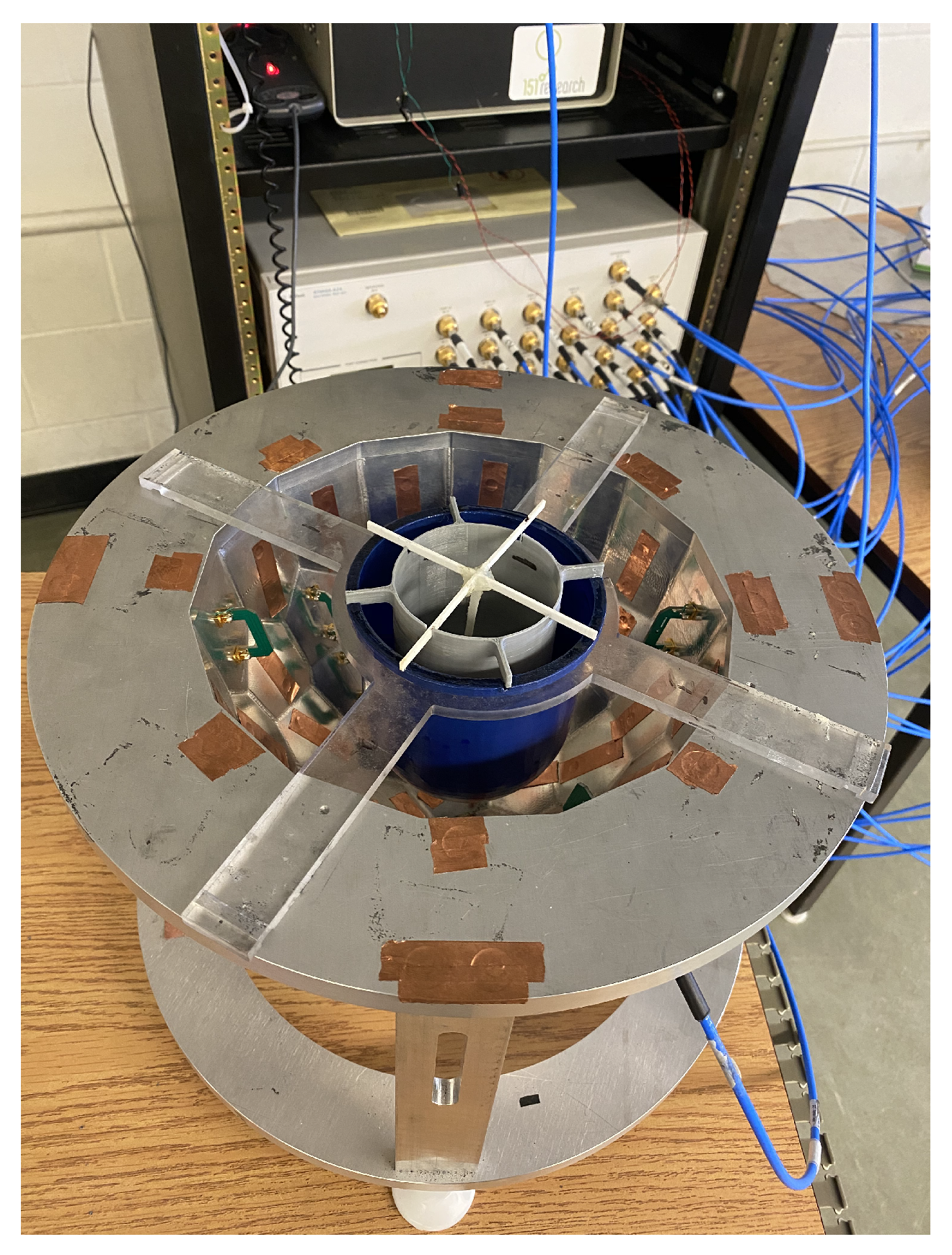
2. Faceted Air-Filled Chamber and Its Model for Microwave Breast Imaging

We have designed our bulk-parameter extraction network around a previously developed breast imaging system that consists of an air-filled quasi-resonant chamber [36]. This chamber is easy to model, available for data collection, and has been studied experimentally [13,37].

The imaging chamber consists of 24 magnetic field probes arranged on its 42 facets. Each field probe in the measurement system acts as a transceiver, resulting in a $24\times 24$ matrix of $S_{i,j}$ measurements, where i is the transmitter index and j is the receiver index. In this system, these S-parameters represent the $\varphi$ projections of the magnetic fields measured at the chamber walls.

We assume that the breast can be placed inside the chamber within a support that would fix the ROI boundary within the imaging chamber (Figure 1).

A full-wave 3-D model of this system is constructed using either of our in-house FEM [14] or DGM [12] solvers, the latter of which supports high-order geometry simplifying modeling of curved regions [38]. These models output H-fields at specified receiver points for each transmitter, where we can convert between S-parameters and H-fields through calibration (details of the transmitter and receiver probe numerical models can be found in [38].

The field data obtained from the system with a breast target is denoted $H_{breast}^{tot}$ (this notation is shared for both S and H). Assuming some prior information of the target, we denote the total-field data for the prior information as $H_{prior}^{tot}$. Scattered fields of the breast relative to the prior information are:

$$H_{target}^{sct}=H_{breast}^{tot}-H_{prior}^{tot}$$

(1)

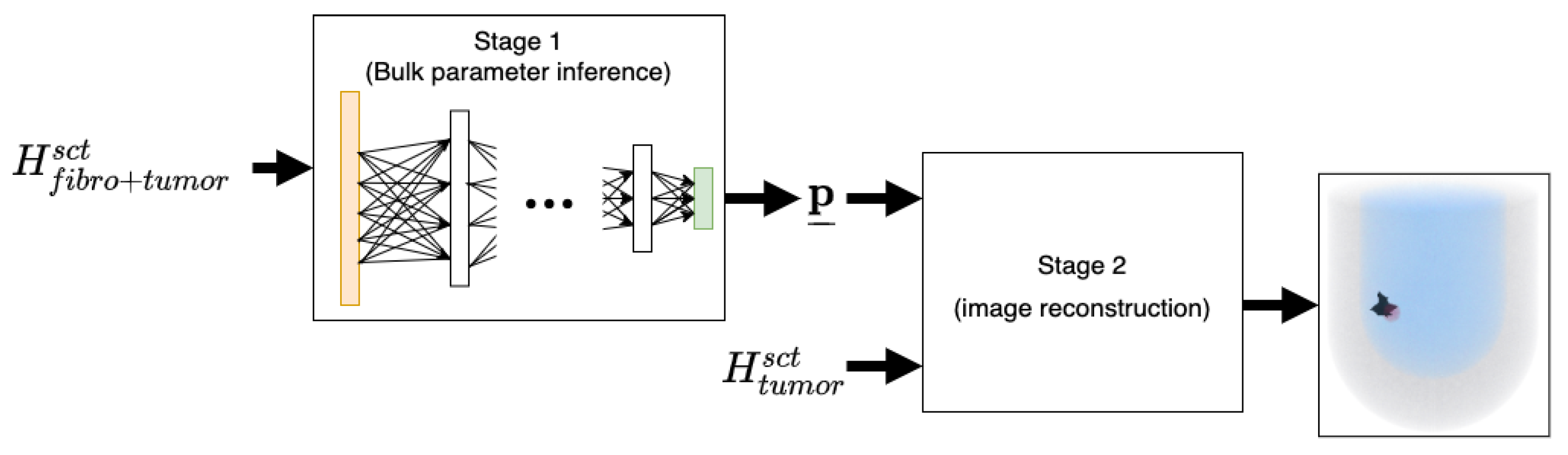
3. A Two-Stage Workflow for Prior Information Extraction and Data Inversion

Imaging multi-wavelength high-contrast targets, such as the human breast in air, is extremely difficult without the use of accurate background information to reduce the contrast in the non-linear imaging problem [4,16]. However, seeking bulk parameters using standard optimization techniques is computationally expensive [33]. As a result of these two facts, we propose a workflow for microwave breast imaging that consists of two distinct stages: Stage 1, bulk parameter (prior information) inference, and Stage 2, image reconstruction. The point is to allow the bulk parameters reconstructed in Stage 1 to serve as prior information for full image reconstruction in Stage 2 as shown in Figure 2. Regardless of the exact nature of the bulk parameters, Stage 1 outputs them as a vector $\underline{\mathbf{p}}$. Both stages of the workflow accept a form of the measurement data from the imaging system, and are described in the following subsections.

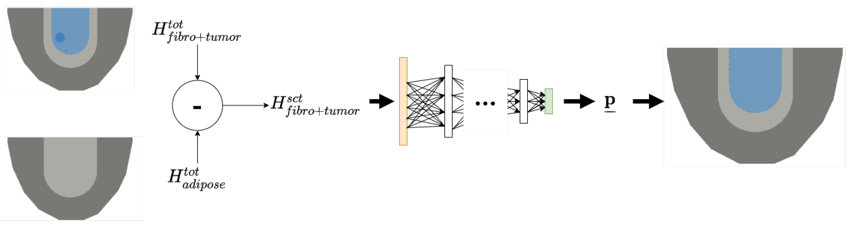
3.1. Stage 1: Bulk Parameter Inference using Neural Networks

The goal of Stage 1 of our two-stage workflow is to estimate bulk parameters of the breast for use as prior information in Stage 2. In this work we choose our bulk parameters to define only the fibroglandular region of the breast, namely its tissue radius, height, and complex-valued permittivity. Thus, our proof-of-concept machine learning model assumes an adipose region of fixed extent, within which exists a centered fibroglandular region of varying size (height and radius). We note that this assumption for the adipose region is not as limiting as it may at first appear as the imaging system can be setup to fix the breast surface and thus the ROI boundary. Future work will consider making this model more flexible. We have chosen to ignore the equivalent of skin in our model, as previous work has shown that inclusion of the skin layer is not critical when attempting to accurately reconstruct the adipose region [39]. However, as shown in [16,17], an approximate skin-layer can be introduced as required to improve the results.

Figure 3 shows renderings of the interior of the imaging chamber for two representative breast models.

For this stage of the workflow, the neural network accepts flattened matrices of data $H_{fibro+tumor}^{sct}$ as input. These fields, as defined in Equation (1), are obtained by taking the difference of total fields $H_{breast}^{tot}$ (which may or may not contain a tumor) and $H_{prior}^{tot}=H_{adipose}^{tot}$, i.e., total fields for the fixed adipose region without the fibroglandular region and without any tumor. The goal is to pass $H_{fibro+tumor}^{sct}$ as an input sample to a trained neural network and have it return the parameters $\underline{\mathbf{p}}$ as shown in Figure 4. By design this parameter extraction does not attempt to detect or localize any tumors, but seeks an approximation to the fibroglandular region that is sufficiently accurate to allow tumor detection in Stage 2 as described in Section 3.2.

3.1.1. Labelled Data

In order to facilitate supervised learning, a large dataset that is representative of data obtained using the experimental setup is required. It is not practical to obtain a large number of labelled experimental measurements from this system, and synthetically generated data must be used. We have previously shown that bulk-parameter networks can be trained on synthetic data and and successfully applied to uncalibrated experimental data [34]. Synthetic data should be chosen to cover a range of expected fibroglandular geometries and permittivities within the fixed adipose region.

When building the training data we can choose whether tumors should be included or excluded from the dataset. The approach taken herein is to exclude tumors from the training set altogether. This has the benefit of not requiring an extensive dataset representative of the many possible variations in tumor properties. Of course this approach necessitates demonstrating that the network is robust to the presence of tumors when predicting bulk parameters. That is, the network should accurately predict the $\underline{\mathbf{p}}$ parameters even from data obtained from phantoms containing tumors.

We have chosen to use single-frequency, phaseless data as Stage 1 input and to ignore back-scatter measurements, i.e., transmitter/receiver pair $(i,i)$. Thus, each labelled sample consists of $(|H_{fibro\left(\underline{\mathbf{p}}\right)}^{sct}|,\underline{\mathbf{p}})$, where $\left|H\right|$ represents the element-wise magnitude of the matrix H, and $H_{fibro\left(\underline{\mathbf{p}}\right)}^{sct}$ is the now $24\times 23$ matrix of scattered fields for the fibroglandular region parameterized by $\underline{\mathbf{p}}$, relative to the assumed known adipose background where the element-wise subtraction in Equation (1) is carried out in the complex domain. In this particular model, the parameter vector $\underline{\mathbf{p}}$ consists of four labels: the radius, height, as well as the real and imaginary parts of the complex-valued permittivity (respectively ${\epsilon }^{\prime }$ and ${\epsilon }^{″}$) for the fibroglandular region.

3.1.2. Stage 1 Network Architecture

The adopted network architecture is a fully-connected neural network. Each input sample, $|H_{fibro+tumor}^{sct}|$ consisting of $24\times 23$ real values, is flattened into a $552\times 1$ vector to be compatible with the network’s 552-node input layer. The rest of the network consists of 5 hidden layers, with a 4-parameter output vector. All layers in the network have rectified linear unit (ReLU) activation. The full network architecture is 552→2048→1024→512→256→64→4 (where the first (552) layer is the input layer and last (4) layer is the output layer). We use a residual sum of squares loss function:

$$\begin{array}{c}\hfill L\left(\underline{\mathbf{p}}\right)=\frac{{(\underline{\mathbf{p}}-{\underline{\mathbf{p}}}_{true})}^T(\underline{\mathbf{p}}-{\underline{\mathbf{p}}}_{true})}{{{\underline{\mathbf{p}}}_{true}}^T{\underline{\mathbf{p}}}_{true}}\end{array}$$

(2)

where ${\underline{\mathbf{p}}}_{true}$ represents the true labels and T denotes the transpose of a vector. To offset the difference in magnitude of the parameter labels and to ensure that each of the four parameters is weighted equally in the loss function, the labels are normalized to zero mean, and unit variance prior to training. Full details on the bulk parameter inference network are available in our previous work [35].

3.1.3. Sample Pre-Processing

Before being passed to the neural network data are passed through a pre-processing step, where the complex measurement data are converted to magnitudes, and normalized by the maximum value on a per-transmitter basis. All test examples are subjected to the same pre-processing steps as the training data (conversion to magnitude-only, and per-transmitter normalization).

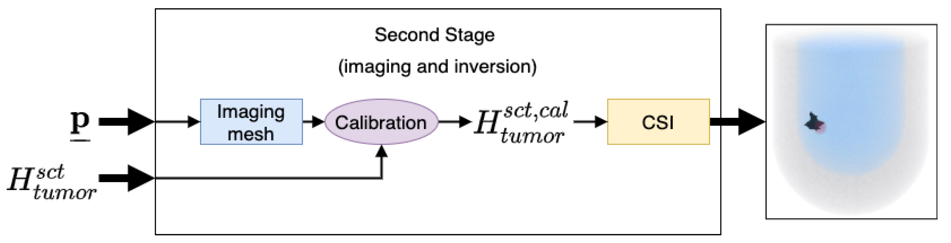
3.2. Stage 2: 3D Image Reconstruction and Tumour Detection

Once Stage 1 of the workflow has provided an estimate of $\underline{\mathbf{p}}$, Stage 2 is applied to detect and/or monitor tumors. In this inversion stage of the workflow, the inputs are the calibrated $H_{tumor}^{sct}=H_{breast}^{tot}-H_{fibro+adipose}^{tot}$. To calculate $H_{tumor}^{sct}$ we have effectively introduced the need for a registered baseline measurement $H_{baseline}^{tot}$, which we take to be $H_{baseline}^{tot}=H_{fibro+adipose}^{tot}$. An appropriate registered baseline measurement implies Stage 1 parameters $\underline{\mathbf{p}}$ that are the same for both $H_{breast}^{tot}$ and $H_{baseline}^{tot}$.

The overall two-stage workflow is summarized in Figure 2, and Figure 5 outlines the second stage of this workflow as presented in this work. The approach used here adopts the CSI algorithm in Stage 2. Previous work has demonstrated the ability of CSI to reconstruct the permittivity profile of the breast model from experimental data assuming accurate prior information is known [16]. Demonstrating that Stage 2 works with imperfect prior obtained from Stage 1 is a significant step towards practicality. Of course many other Stage 2 approaches are also possible, i.e., any other inversion algorithm or a machine learning approach.

Contrast Source Inversion

CSI is a well-known iterative approach to solving the non-linear inverse scattering problem [40]. Our implementation of CSI used for this work is based on a partial differential equation formulations of Maxwell’s equations namely the finite element method (FEM-CSI). This algorithm easily supports prior information in the form of inhomogeneous backgrounds, details can be found in [14,41]. The parameters obtained from the neural network, $\underline{\mathbf{p}}$, are used as prior information for the inversion where the fibroglandular region height and radius predictions are used to generate a new model for which a forward solver is called to generate $H_{fibro\left(\underline{\mathbf{p}}\right)+adipose}^{tot}$ data for this tissue geometry, where the permitivitty of the fibroglandular region used for the forward solver is the complex-valued permittivity prediction from $\underline{\mathbf{p}}$. The background physics for the CSI inversion are then taken to be the assumed known complex-valued permittivity for adipose tissue, and the $\underline{\mathbf{p}}$ predicted complex-valued permittivity for fibroglandular tissue. An imaging model is generated according to these parameters, whose discretization is intentionally different from that used to generate the forward data for the test examples.

CSI seeks to reconstruct regions of contrast with respect to the provided prior background.As discussed in Section 3.2 we currently assume that the background is characterized by the baseline measurement of the breast in which the field measurements of the adipose and fibroglandular regions of the breast are known. In this configuration, CSI should reconstruct the tumor.

3.3. Calibration

As forward model discretization can result in significant simulated field errors relative to the scattering signature of the target, it is necessary to calibrate the test data to the imaging model (CSI prior information) to eliminate errors arising from the use of different models. The calibrated scattered fields are computed as

$$H_{target}^{cal}=\frac{H_{prior}^{tot}}{H_{baseline}^{tot}}(H_{breast}^{tot}-H_{baseline}^{tot})$$

(3)

where $H_{prior}^{tot}=H_{fibro\left(\underline{\mathbf{p}}\right)+adipose}^{tot}$ is the total field forward data for the prior information (imaging) model, and $H_{breast}^{tot}$ and $H_{baseline}^{tot}=H_{fibro+adipose}^{tot}$.

4. Results

In what follows we demonstrate the proposed two-stage workflow on synthetic data. Initial testing on experimental data shows that Stage 1 is capable of recovering the geometry of the fibroglandular region.

4.1. Data Generation

A synthetic model of the air-filled chamber described in Section 2 was created. To simplify the model and speed up synthetic data generation, we elected to set the top plane of the system to a perfect electric conductor (PEC). We note that in practice an impedance boundary condition may be more appropriate for modelling the patient chest wall across the top surface of the chamber. In the model, the 24 magnetic field probes, when transmitting, are approximated as 24 magnetic dipole sources placed tangential to the appropriate chamber facet that correspond to their location in the experimental system.

The synthetic data used for training and evaluating the network was generated using a high-order Discontinuous Galerkin Method (DGM) forward solver [12,38]. In all cases, second-order mesh geometry and third-order field solutions were used.

Data was generated at 1.1 GHz, corresponding to a freespace wavelength of around 27 cm or roughly 1.2 times the radius at the top of the chamber. Each of the tissue types considered in this model were characterized based on an approximation of their complex-valued permittivity at 1.1 GHz: in all cases adipose was assigned a permittivity of $3-j0.6$, and tumors were assigned a permittivity of $56.3-j30$ [32]. As we have previously assumed that the experimental imaging system can be designed with a support that would fix the overall size and shape of the target to known geometry, for all synthetic training examples the size of the adipose region was fixed with a height of 10.9 cm and a radius of 4.8 cm.

To create a labelled dataset, synthetic breast models were generated for varying fibroglandular region heights and radii ranging from 5.30 to 9.80 cm and 2.85 to 4.10 cm, and for a wide range of complex-valued bulk permittivities for the fibroglandular tissue: the real part of the permittivity ranged from 15 to 25 and the imaginary part of the permittivity ranged from −25 to −15. The range of values used to generate the labelled dataset are summarized in

Table 1. Summary of fibroglandular region variations in the labelled dataset.

Radius Range [cm]	Height Range [cm]	${\mathit{\epsilon }}^{\prime }$ Range	${\mathit{\epsilon }}^{\prime \prime }$ Range
[2.85, 4.10]	[5.30, 9.80]	[15, 25]	[−25, −15]

.

The labelled dataset consists of a total of 7116 tumor-free examples, which are partitioned into training, validation and reserved test sets of 85%, 10%, and 5% of the set, respectively. Tumors were intentionally omitted from all training examples so that we could later evaluate the robustness of the Stage 1 network to the presence of tumors.

Table 2. Summary of error in predictions for the noise-free synthetic test set.

Metric	Error in	Error in	Error in	Error in
	Radius [mm]	Height [mm]	${\mathit{\epsilon }}^{\prime }$	${\mathit{\epsilon }}^{\prime \prime }$
Average absolute error	0.0280	0.0248	0.0866	0.0963
Average absolute error (%)	0.97%	0.83%	0.58%	0.39%
Standard deviation	0.0204	0.0194	0.0670	0.0765

shows the average absolute error and standard deviation in each parameter for the testing set comprised of 5% of the noise-free synthetic examples described above.

4.2. Tumor Detection Test Samples

In addition to the tumor-free labelled dataset described above, synthetic data was generated for three unique geometries representing small, medium, and large fibroglandular regions. For these unique geometries, one baseline (tumor-free), and two tumor-containing examples were generated, where the tumor is a spherical target with a radius of 9 mm. In each tumor-containing example, the target was placed at one of two different locations within the fibroglandular region. For the medium fibroglandular case, data was also generated for a 4.5 mm radius tumor. In all cases the complex-valued permittivity of the fibroglandular region was set to be $20-j21.6$ [32]. A single fibroglandular permittivity was chosen to reduce the problem size for this proof of concept workflow, and the particular value was selected to correspond to an existing experimental phantom. This data corresponds to different examples of $H_{breast}^{tot}$. To simulate measurement noise, white Gaussian noise between. $\pm {10}^{-4}\ast \max real\left(\right|H_{breast}^{tot}\left|\right)$ and $\pm {10}^{-4}\ast \max imag\left(\right|H_{breast}^{tot}\left|\right)$ was applied to the real and imaginary parts of the data, respectively, where ${10}^{-4}$ represents −80 dB noise for the total field data.

4.3. Parametric Inference of Fibroglandular Region Parameters

Using the training set, a single frequency, magnitude-only (phaseless) neural network, described in Section 3.1.2 was trained to perform bulk parameter inference. The model was generated using Python and TensorFlow Keras. This neural network was trained with a batch size of 100, for a maximum of 150 epochs with an early stopping patience of 30 iterations.

The ability of the neural network to predict the geometry and complex permittivity of the fibroglandular region was evaluated for synthetic cases with and without a tumour. In all cases the output of the network, $\underline{\mathbf{p}}$, describes only the fibroglandular region, and does not directly provide any information on the presence, size, or location of the tumor.

Table 3. Summary of fibroglandular parameter predictions for synthetic examples with −80 dB noise.

Position	Tumor Radius	Radius	Height	${\mathit{\epsilon }}^{\prime }$	${\mathit{\epsilon }}^{\prime \prime }$
	[mm]	[cm]	[cm]
Small fibroglandular case:
True values: ${\underline{\mathbf{p}}}_{true}$		2.90	5.35	20.0	−21.6
No tumor	-	3.06	6.04	16.02	−21.85
T1	9	3.05	6.09	16.66	−22.08
T2	9	3.06	6.13	16.03	−22.07
Medium fibroglandular case:
True values: ${\underline{\mathbf{p}}}_{true}$		3.40	8.50	20.0	−21.6
No tumor	-	3.39	8.46	19.90	−21.60
T1	9	3.39	8.47	19.71	−21.72
T1	4.5	3.40	8.44	20.03	−21.57
T2	9	3.39	8.45	20.48	−21.58
Large fibroglandular case:
True values: ${\underline{\mathbf{p}}}_{true}$		4.05	9.75	20.0	−21.6
No tumor	-	4.07	9.71	19.81	−21.55
T1	9	4.07	9.73	19.74	−21.36
T2	9	4.06	9.72	19.79	−21.58

presents the output of the neural network for three different fibroglandular region sizes, each with two different tumor positions. The true value of the parameters is provided for reference. For the medium fibroglandular case, two different sized tumors were tested at position one. All tumors are spherical, with radius as specified in column two of the table.

The results in Table 3 suggest that the neural network may be capable of accurately predicting the prior information needed for CSI. It also shows that the network is robust to the presence of tumors of different sizes and locations for the medium and large fibroglandular regions. The neural network is not as successful in reconstructing the bulk parameters when the fibroglandular region is small relative to the size of the fat region.

To further evaluate the impacts of noise on the parameter predictions from Stage 1, each of the test cases in Table 3 was evaluated for −40 dB and −60 dB noise (in addition to the −80 dB noise presented above).

Table 4. Summary of error in predictions for the noisy, tumor-containing test cases.

Noise	Metric	Error in	Error in	Error in	Error in
		Radius [mm]	Height [mm]	${\mathit{\epsilon }}^{\prime }$	${\mathit{\epsilon }}^{\prime \prime }$
${10}^{-4}$	Average	0.0545	0.0251	1.28	0.167
(−80 dB)	Max	0.161	0.775	3.98	0.478
${10}^{-3}$	Average	0.0549	0.0250	1.41	0.283
(−60 dB)	Max	0.180	0.779	4.56	0.679
${10}^{-2}$	Average	0.115	0.444	4.06	2.92
(−40 dB)	Max	0.233	1.31	7.47	10.1

shows the average and maximum absolute error for each parameter across the 10 tumor-containing, noisy test cases. These results demonstrate that the network remains robust to noise when the noise applied is increased from −80 dB to −60 dB. For −40 dB noise the network still gives reasonable results, but the prediction error begins to increase and in the case of the complex-valued permittivity predictions, the maximum error is nearly half of the true value.

Figure 6 shows the neural network prediction versus true prior information for the 9 mm tumor in position T1 for each fibroglandular size.

4.4. CSI-Based Tumor Detection from Predicted Prior Information

To demonstrate that the output of the Stage 1 network is accurate enough to be used as prior information for CSI, the parameters, $\underline{\mathbf{p}}$, extracted by the network for the tumor detection test samples were used as prior information for CSI reconstructions of the fibroglandular region, where the goal is to detect and localize the tumor. For each test example, CSI was run to recover the tumor (high contrast region). The test sample data was calibrated according to the procedure outlined in Section 3.3. The synthetic test data is generated using a completely independent forward solver that was used to create the training set data. Therefore, although counter-intuitive, the calibration procedure, which is typically used to calibrate experimental data to the numerical inverse model, must also be applied to the synthetic test data set. This effectively calibrates data obtained from one modelling engine (the DGM forward solver in this case), with it’s own inherent systematic errors (such as mesh error), to the training set data obtained via a different modelling engine (the FEM forward solver in the present case). Figure 7 shows the reconstruction of the tumor in two different positions within each size of fibroglandular region superimposed on the true prior. To visualize the tumor, the real part of the recovered contrast, $\chi$, was thresholded at 85% of the maximum reconstructed contrast for the given test example, these thresholded regions are superimposed on the true real permittivity map of the model (Figure 7). This result shows that when using prior information obtained from the Stage 1 neural network, the approximate location of a tumor within the breast model can be determined.

As the intent of this work is to demonstrate the ability to distinguish the tumor tissue from the background, and not necessarily to accurately determine the permittivity, CSI was terminated after relatively few (200) iterations. A consequence of this choice is that permittivity reconstruction is consistently lower than expected. Running CSI for more iterations, and applying post-processing to the images using deep learning has been shown to improve the artifact prone, low contrast inversions shown in Figure 7 [32].

4.5. Monitoring Response to Tumor Treatment

Figure 8 shows the imaging results for the T1 tumor (fixed position) with two different tumor sizes, compared with the imaging result for the tumor-free case. The CSI reconstruction of the data for these two different tumor sizes shows a decrease in the size and recovered contrast of the region identified as a tumor with a decrease in tumor size in the forward problem. This result suggests that the proposed workflow may be useful in monitoring tumor response to treatment, where the most recent image of the tumor is used as baseline prior information.

4.6. Preliminary Bulk Parameter Inference Results on Experimental Data

A limited set of experimental data obtained from the system as described in [13] was evaluated using a similar bulk parameter inference network. The experimental breast phantom consisted of a phantom that fits our general description of fibroglandular and adipose tissues (e.g., Figure 3), with tissue mimicking fluids filling each region in thin-walled containers (see Figure 1). Two measurements were taken with only adipose and fibroglandular regions and two measurements were taken with a tumor in the fibroglandular region in two different locations.

Forward data was generated for the same parameters and ranges as outlined in Table 1. The experimental data was collected with an open top, and thus the flat PEC top model used for the synthetic results presented above is unsuitable. Instead, to model the experimental setup, the imaging system model was modified such that the region above the top surface of the chamber is air, where an absorbing boundary condition is applied. In order to keep the model discretization manageable for timely labelled dataset generation, the absorbing boundary condition was left in relative close proximity to the chamber’s PEC surfaces limiting the model’s accuracy. New data was generated according to this model to train a neural network of the same architecture described in Section 3.1.2. The new synthetic dataset consists of 25,409 labelled examples (partitioned 85%, 10%, 5% into training, validation, and test sets, respectively). Prior to being passed as inputs to the neural network, the experimental measurements were calibrated to the synthetic data as scattered fields relative to a measured adipose model background. For experimental data, these background measurements were obtained by filling the phantoms with canola oil. The full process for experimental data collection is described in [13].

Table 5. Summary of fibroglandular region parameter predictions for calibrated experimental examples.

Position	Tumor Radius	Radius	Height	${\mathit{\epsilon }}^{\prime }$	${\mathit{\epsilon }}^{\prime \prime }$
	[mm]	[cm]	[cm]
True values: ${\underline{\mathbf{p}}}_{true}$		3.40	8.50	20.0	−21.6
No tumor 1	-	3.50	8.39	13.37	−14.24
No tumor 2	-	3.47	8.29	13.38	−14.85
T1	9	3.56	8.56	11.83	−15.38
T2	9	3.55	8.25	11.61	−16.35

provides preliminary predictions of $\underline{\mathbf{p}}$ for experimental data.

These results show that, for the appropriate synthetic training set, the Stage 1 network architecture outlined in this work is capable of recovering the fibroglandular geometry information with reasonable accuracy. In these preliminary results, the neural network undershoots the complex-valued permittivity predictions, which may be due to the accuracy of the absorbing boundary condition used when generating the training set. Further research is ongoing to determine ways to improve the results for experimental data.

5. Conclusions

We have presented a framework for microwave imaging that is capable of detecting the presence of, and monitoring the size of tumors in a model of the human breast. This framework can accept electromagnetic field measurements and through a two-stage process can predict the bulk parameters of the fibroglandular region within the breast and use that as prior information for a 3D inversion of the field data to reconstruct regions of high complex-valued permittivity compared to some known tissue background within the breast. Although the bulk parameter predictions from the Stage 1 neural network do not represent perfect prior information, the results presented in this work show that an inversion algorithm is still capable of detecting the presence of a tumor and determining its approximate size and location within the fibroglandular region of the breast based on the predicted (imperfect) prior information.

While we have demonstrated the success of a two-stage workflow for obtaining prior information and performing inversion on microwave breast imaging data, further research is required to assess the success of this framework, and particularly the bulk parameter inference neural network, for experimental data. The breast model presented in this work is relatively simple, assuming uniformly shaped tissue regions and considering only a single tumor case. An interesting focus of future work would be to investigate the performance of this framework for a more complicated model of the breast, or one with multiple tumors. A limitation of this work is that the permittivity reconstructions obtained through 200 iterations of CSI are consistently low. Our current focus is to try and improve the permittivity reconstruction accuracy through more iterations of CSI combined with a deep-learning post-processing step [32] to improve the overall quality of the output image.

References

1. Conceição, R.C.; Mohr, J.J.; O’Halloran, M. An Introduction to Microwave Imaging for Breast Cancer Detection; Springer: Berlin/Heidelberg, Germany, 2016. [Google Scholar]
2. Nikolova, N.K. Microwave imaging for breast cancer. IEEE Microw. Mag. 2011, 12, 78–94. [Google Scholar] [CrossRef]
3. Omer, M.; Mojabi, P.; Kurrant, D.; LoVetri, J.; Fear, E. Proof-of-concept of the incorporation of ultrasound-derived structural information into microwave radar imaging. IEEE J. Multiscale Multiphys. Comput. Tech. 2018, 3, 129–139. [Google Scholar] [CrossRef]
4. Neira, L.M.; Van Veen, B.D.; Hagness, S.C. High-resolution microwave breast imaging using a 3-D inverse scattering algorithm with a variable-strength spatial prior constraint. IEEE Trans. Antennas Propag. 2017, 65, 6002–6014. [Google Scholar] [CrossRef]
5. Poplack, S.P.; Tosteson, T.D.; Wells, W.A.; Pogue, B.W.; Meaney, P.M.; Hartov, A.; Kogel, C.A.; Soho, S.K.; Gibson, J.J.; Paulsen, K.D. Electromagnetic breast imaging: Results of a pilot study in women with abnormal mammograms. Radiology 2007, 243, 350–359. [Google Scholar] [CrossRef] [Green Version]
6. Catapano, I.; Di Donato, L.; Crocco, L.; Bucci, O.M.; Morabito, A.F.; Isernia, T.; Massa, R. On quantitative microwave tomography of female breast. Prog. Electromagn. Res. 2009, 97, 75–93. [Google Scholar] [CrossRef] [Green Version]
7. Abdollahi, N.; Kurrant, D.; Mojabi, P.; Omer, M.; Fear, E.; LoVetri, J. Incorporation of ultrasonic prior information for improving quantitative microwave imaging of breast. IEEE J. Multiscale Multiphys. Comput. Tech. 2019, 4, 98–110. [Google Scholar] [CrossRef]
8. Ambrosanio, M.; Kosmas, P.; Pascazio, V. A Multithreshold Iterative DBIM-Based Algorithm for the Imaging of Heterogeneous Breast Tissues. IEEE Trans. Biomed. Eng. 2019, 66, 509–520. [Google Scholar] [CrossRef]
9. Benny, R.; Anjit, T.A.; Mythili, P. An overview of microwave imaging for breast tumor detection. Prog. Electromagn. Res. 2020, 87, 61–91. [Google Scholar] [CrossRef]
10. Lazebnik, M.; Popovic, D.; McCartney, L.; Watkins, C.B.; Lindstrom, M.J.; Harter, J.; Sewall, S.; Ogilvie, T.; Magliocco, A.; Breslin, T.M.; et al. A large-scale study of the ultrawideband microwave dielectric properties of normal, benign and malignant breast tissues obtained from cancer surgeries. Phys. Med. Biol. 2007, 52, 6093. [Google Scholar] [CrossRef]
11. Shea, J.D.; Kosmas, P.; Hagness, S.C.; Van Veen, B.D. Three-dimensional microwave imaging of realistic numerical breast phantoms via a multiple-frequency inverse scattering technique. Med. Phys. (Lancaster) 2010, 37, 4210–4226. [Google Scholar] [CrossRef]
12. Brown, K.G.; Geddert, N.; Asefi, M.; LoVetri, J.; Jeffrey, I. Hybridizable discontinuous Galerkin method contrast source inversion of 2-D and 3-D dielectric and magnetic targets. IEEE Trans. Microw. Theory Tech. 2019, 67, 1766–1777. [Google Scholar] [CrossRef]
13. Asefi, M.; Baran, A.; LoVetri, J. An Experimental Phantom Study for Air-Based Quasi-Resonant Microwave Breast Imaging. IEEE Trans. Microw. Theory Tech. 2019, 67, 3946–3954. [Google Scholar] [CrossRef]
14. Zakaria, A.; Jeffrey, I.; LoVetri, J.; Zakaria, A. Full-vectorial parallel finite-element contrast source inversion method. Prog. Electromagn. Res. 2013, 142, 463–483. [Google Scholar] [CrossRef] [Green Version]
15. Tournier, P.H.; Bonazzoli, M.; Dolean, V.; Rapetti, F.; Hecht, F.; Nataf, F.; Aliferis, I.; El Kanfoud, I.; Migliaccio, C.; De Buhan, M.; et al. Numerical Modeling and High-Speed Parallel Computing: New Perspectives on Tomographic Microwave Imaging for Brain Stroke Detection and Monitoring. IEEE Antennas Propag. Mag. 2017, 59, 98–110. [Google Scholar] [CrossRef] [Green Version]
16. Kurrant, D.; Baran, A.; LoVetri, J.; Fear, E. Integrating prior information into microwave tomography Part 1: Impact of detail on image quality. Med. Phys. 2017, 44, 6461–6481. [Google Scholar] [CrossRef]
17. Kurrant, D.; Fear, E.; Baran, A.; LoVetri, J. Integrating prior information into microwave tomography part 2: Impact of errors in prior information on microwave tomography image quality. Med. Phys. (Lancaster) 2017, 44, 6482–6503. [Google Scholar] [CrossRef]
18. Golnabi, A.H.; Meaney, P.M.; Paulsen, K.D. Tomographic microwave imaging with incorporated prior spatial information. IEEE Trans. Microw. Theory Tech. 2013, 61, 2129–2136. [Google Scholar] [CrossRef]
19. Bevacqua, M.T.; Bellizzi, G.G.; Isernia, T.; Crocco, L. A method for effective permittivity and conductivity mapping of biological scenarios via segmented contrast source inversion. Prog. Electromagn. Res. 2019, 164, 1–15. [Google Scholar] [CrossRef] [Green Version]
20. Abdollahi, N.; Jeffrey, I.; LoVetri, J. Improved Tumor Detection via Quantitative Microwave Breast Imaging Using Eigenfunction-Based Prior. IEEE Trans. Comput. Imaging 2020, 6, 1194–1202. [Google Scholar] [CrossRef]
21. Hughson, M.; Jeffrey, I.; LoVetri, J. Ultrasound and Microwave Imaging with Prior Property Dependencies. In Proceedings of the 2019 IEEE MTT-S International Conference on Numerical Electromagnetic and Multiphysics Modeling and Optimization (NEMO), Boston, MA, USA, 29–31 May 2019; pp. 1–4. [Google Scholar]
22. Obermeier, R.; Martinez-Lorenzo, J.A. Compressive sensing unmixing algorithm for breast cancer detection. IET Microw. Antennas Propag. 2018, 12, 533–541. [Google Scholar] [CrossRef]
23. Chen, X. Computational Methods for Electromagnetic Inverse Scattering; John Wiley & Sons Pte. Ltd.: Singapore, 2018. [Google Scholar]
24. Wei, Z.; Chen, X. Deep-learning schemes for full-wave nonlinear inverse scattering problems. IEEE Trans. Geosci. Remote Sens. 2018, 57, 1849–1860. [Google Scholar] [CrossRef]
25. Li, L.; Wang, L.; Teixeira, F.; Che, L.; Cui, T. DeepNIS: Deep Neural Network for Nonlinear Electromagnetic Inverse Scattering. IEEE Trans. Antennas Propag. 2018. [Google Scholar] [CrossRef] [Green Version]
26. Guo, R.; Song, X.; Li, M.; Yang, F.; Xu, S.; Abubakar, A. Supervised descent learning technique for 2-D microwave imaging. IEEE Trans. Antennas Propag. 2019, 67, 3550–3554. [Google Scholar] [CrossRef]
27. Oktay, O.; Ferrante, E.; Kamnitsas, K.; Heinrich, M.P.; Bai, W.; Caballero, J.; Guerrero, R.; Cook, S.A.; de Marvao, A.; Dawes, T.; et al. Anatomically Constrained Neural Networks (ACNN): Application to Cardiac Image Enhancement and Segmentation. IEEE Trans. Med. Imaging 2017, 37, 384–395. [Google Scholar] [CrossRef] [Green Version]
28. Shao, W.; Du, Y. Microwave Imaging by Deep Learning Network: Feasibility and Training Method. IEEE Trans. Antennas Propag. 2020, 68, 5626–5635. [Google Scholar] [CrossRef]
29. Chen, X.; Wei, Z.; Li, M.; Rocca, P. A Review of Deep Learning Approaches for Inverse Scattering Problems (Invited Review). Prog. Electromagn. Res. 2020, 167, 67–81. [Google Scholar] [CrossRef]
30. Khoshdel, V.; Ashraf, A.; LoVetri, J. Enhancement of Multimodal Microwave-Ultrasound Breast Imaging Using a Deep-Learning Technique. Sensors 2019, 19, 4050. [Google Scholar] [CrossRef] [Green Version]
31. Mojabi, P.; Khoshdel, V.; LoVetri, J. Tissue-Type Classification With Uncertainty Quantification of Microwave and Ultrasound Breast Imaging: A Deep Learning Approach. IEEE Access 2020, 8, 182092–182104. [Google Scholar] [CrossRef]
32. Khoshdel, V.; Asefi, M.; Ashraf, A.; LoVetri, J. Full 3D Microwave Breast Imaging Using a Deep-Learning Technique. J. Imaging 2020, 6, 80. [Google Scholar] [CrossRef]
33. Gilmore, C.; Jeffrey, I.; Asefi, M.; Geddert, N.T.; Brown, K.G.; LoVetri, J. Phaseless Parametric Inversion for System Calibration and Obtaining Prior Information. IEEE Access 2019, 7, 128735–128745. [Google Scholar] [CrossRef]
34. Edwards, K.; Krakalovich, K.; Kruk, R.; Khoshdel, V.; LoVetri, J.; Gilmore, C.; Jeffrey, I. The implementation of neural networks for phaseless parametric inversion. In Proceedings of the 2020 XXXIIIrd General Assembly and Scientific Symposium of the International Union of Radio Science, Rome, Italy, 29 August–5 September 2020; pp. 1–3. [Google Scholar]
35. Edwards, K.; Geddert, N.; Krakalovich, K.; Kruk, R.; Asefi, M.; Lovetri, J.; Gilmore, C.; Jeffrey, I. Stored Grain Inventory Management Using Neural-Network-Based Parametric Electromagnetic Inversion. IEEE Access 2020, 8, 207182–207192. [Google Scholar] [CrossRef]
36. Nemez, K.; Asefi, M.; Baran, A.; LoVetri, J. A faceted magnetic field probe resonant chamber for 3D breast MWI: A synthetic study. In Proceedings of the 2016 17th International Symposium on Antenna Technology and Applied Electromagnetics (ANTEM), Montreal, QC, Canada, 10–13 July 2016; pp. 1–3. [Google Scholar]
37. Nemez, K.; Baran, A.; Asefi, M.; LoVetri, J. Modeling error and calibration techniques for a faceted metallic chamber for magnetic field microwave imaging. IEEE Trans. Microw. Theory Tech. 2017, 65, 4347–4356. [Google Scholar] [CrossRef]
38. Geddert, N. An electromagnetic hybridizable discontinuous Galerkin method forward solver with high-order geometry for inverse problems. Master’s Thesis, Department of Electrical and Computer Engineering, University of Manitoba, Winnipeg, MB, Canada, 2020. [Google Scholar]
39. Gilmore, C.; Zakaria, A.; Pistorius, S.; LoVetri, J. Microwave imaging of human forearms: Pilot study and image enhancement. Int. J. Biomed. Imaging 2013, 2013, 673027. [Google Scholar] [CrossRef]
40. Van Den Berg, P.M.; Kleinman, R.E. A contrast source inversion method. Inverse Probl. 1997, 13, 1607. [Google Scholar] [CrossRef]
41. Zakaria, A.; Gilmore, C.; LoVetri, J. Finite-element contrast source inversion method for microwave imaging. Inverse Probl. 2010, 26, 115010. [Google Scholar] [CrossRef] [Green Version]
Figure 1. Photograph of the experimental setup with breast phantoms.
Electronics 10 00674 g001
Figure 2. Bulk parametric inversion of scattered-field data to recover prior information (our vector of parameters p ̲ ), followed by data-to-image reconstruction using neural network recovered prior information.
Electronics 10 00674 g002
Figure 3. Renderings of interior of faceted air-filled chamber (a,b) and cross-section (c,d) showing the three regions: air (grey), fat (dark blue), fibroglandular (light blue), for a medium (left) and small (right) fibroglandular region.
Electronics 10 00674 g003
Figure 4. The Stage 1 bulk parameter inference network accepts breast-target data which may include a tumor, and outputs the bulk fibroglandular parameters.
Electronics 10 00674 g004
Figure 5. Workflow stage 2 employing CSI, where p ̲ is obtained from the bulk parameter inference network (first stage), and specifies the fibroglandular region in the imaging mesh.
Electronics 10 00674 g005
Figure 6. True values (left) versus neural network predictions (right) for the fibroglandular region for the T1 test examples for the (a) small fibroglandular case, (b) medium fibroglandular case, and (c) large fibroglandular case. The associated differences in the predicted complex-valued permittivity are provided in Table 3.
Electronics 10 00674 g006
Figure 7. CSI reconstructions for two different tumor positions, when prior information has been generated by our neural network. +z projection (left) and +x projection (right) are shown. (a,b) show T1 and T2 for the small fibroglandular case; (ce) show T1 (9 mm), T2, and the T1 (4.5 mm) for the medium fibroglandular case; (f,g) show T1 and T2 for the large fibroglandular case. Adipose (grey), fibroglandular (blue), and tumor (red) show the true geometry of the breast model tissues. The 85% thresholded contrast representing the reconstructed tumor is shown in black.
Electronics 10 00674 g007
Figure 8. Point cloud representation of the CSI reconstruction of the real and imaginary parts of the complex contrast for the fibroglandular region for the T1 test examples with (a,d) a 9 mm tumor at position T1, (b,e) a 4.5 mm tumor at position T1, and (c,f) no tumor.
Electronics 10 00674 g008