Article

Design and Evaluation of a New Machine Learning Framework for IoT and Embedded Devices

by
Gianluca Cornetta
1,* and
Abdellah Touhafi
2
1
Department of Information Engineering, San Pablo-CEU University, Boadilla del Monte, 28668 Madrid, Spain
2
Department of Engineering Technology (INDI), Vrije Universiteit Brussel, 1050 Brussels, Belgium
*
Author to whom correspondence should be addressed.
Electronics 2021, 10(5), 600; https://doi.org/10.3390/electronics10050600
Submission received: 4 January 2021 / Revised: 26 February 2021 / Accepted: 26 February 2021 / Published: 4 March 2021
(This article belongs to the Special Issue Embedded IoT: System Design and Applications)

Abstract

:
Low-cost, high-performance embedded devices are proliferating and a plethora of new platforms are available on the market. Some of them either have embedded GPUs or the possibility to be connected to external Machine Learning (ML) algorithm hardware accelerators. These enhanced hardware features enable new applications in which AI-powered smart objects can effectively and pervasively run in real-time distributed ML algorithms, shifting part of the raw data analysis and processing from cloud or edge to the device itself. In such context, Artificial Intelligence (AI) can be considered as the backbone of the next generation of Internet of the Things (IoT) devices, which will no longer merely be data collectors and forwarders, but really “smart” devices with built-in data wrangling and data analysis features that leverage lightweight machine learning algorithms to make autonomous decisions on the field. This work thoroughly reviews and analyses the most popular ML algorithms, with particular emphasis on those that are more suitable to run on resource-constrained embedded devices. In addition, several machine learning algorithms have been built on top of a custom multi-dimensional array library. The designed framework has been evaluated and its performance stressed on Raspberry Pi III- and IV-embedded computers.

1. Introduction

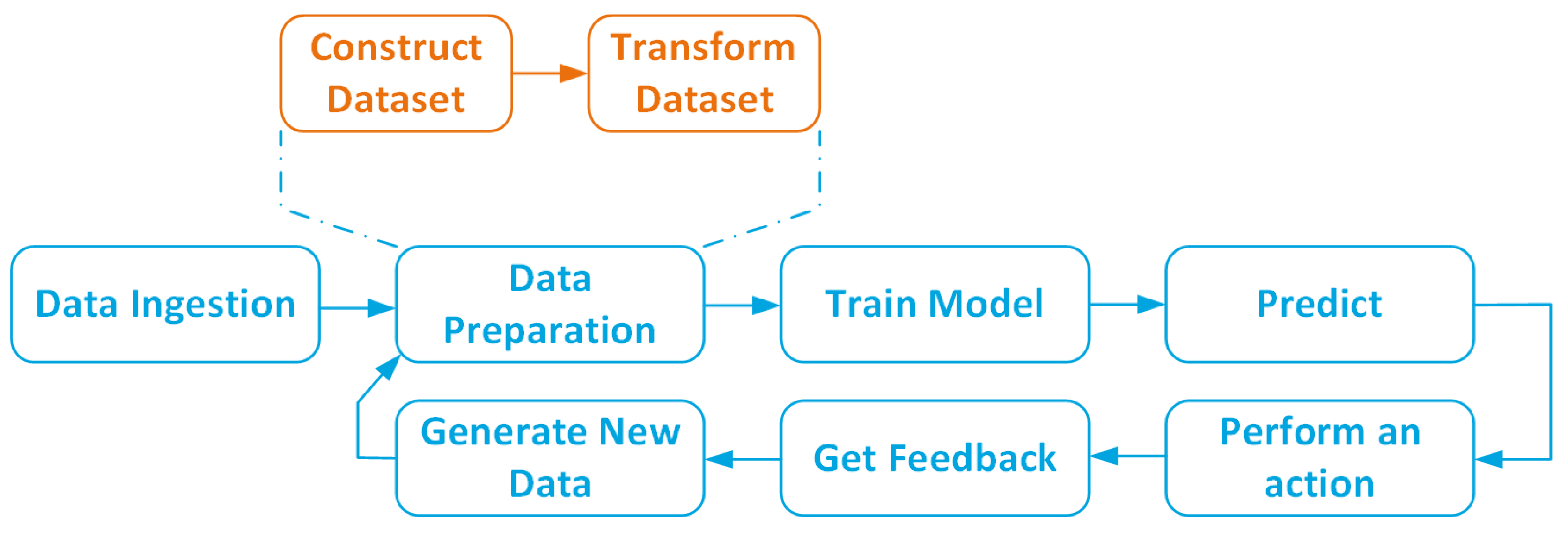
The Internet of Things (IoT) and Artificial Intelligence (AI) are probably two of the most popular research topics at present, driving the interest of both the academic and industrial sectors. The reason for this is their transversality, which makes them suitable for almost every existing application. IoT and AI have been successfully applied to several research and industrial fields, including health  [1], life science [2], smart cities [3,4], environmental monitoring [5,6], precision agriculture [7,8], and education [4,9]. Figure 1 depicts the Machine Learning (ML) adoption process, used to target several kinds of problem or application. Machine learning can be effectively used to:
  • Perform an a posteriori analysis of a given problem in order to detect business process issues and perform optimisation tasks;
  • Gain more insight into a given problem or improve business processes by automating simple and repetitive tasks and assisting the end user in the decision-making process;
  • Perform long-term optimisation by fully automating all the business processes and applying complex predictive techniques.
Both IoT and AI can be considered empowering technologies and, as such, they can converge into a unique framework that leverages their symbiotic relationship to improve, optimise and automate almost every business process.
Moreover, the rapid development of new hardware, software and communication technologies experienced in recent years has fostered the proliferation of low-cost devices and asynchronous communication protocols based on publish/subscribe mechanisms such as Message Queue Telemetry Transport (MQTT) and Constrained Application Protocol (CoAP), which are particularly suitable for IoT applications.
The new sensory boards available on the market now have enough computing power to run locally complex tasks, thus extending the dew computing paradigm to smart objects [11] and allowing for local processing and storage of the measured data before making them available to edge or cloud infrastructure for further processing and analysis.
According to a recent forecast (Source International Data Corporation (IDC), report available on-line at https://www.idc.com/getdoc.jsp?containerId=prUS45213219 (accessed on 10 February 2021)), by 2025, there will be 41.6 billion connected IoT devices generating 79.4 zettabytes (ZB) of data. Thus, IoT will be among the most significant data sources in the upcoming years. However, the effective management of data generated by IoT is not the only concern; besides data volume, IoT is also characterised by the extremely dynamic nature of its data. More specifically, IoT generates time-dependent geolocalised data with a variety of formats, modalities and amounts. Extracting knowledge from such a large amount of time-dependent and heterogeneous data is a challenging task. In this new, data-centric context, data science and AI will play a crucial role.
Data science is the combination of several scientific fields relying on data-mining, big data, machine learning and statistical techniques, aimed at making meaningful raw data through pattern matching.
Data analysis is the process of inspecting, cleansing and modelling data, and involves several steps, from data wrangling (namely, remapping raw data into another format more suitable for analysis), identification of the data attributes (either categorical or quantitative) and choice of a suitable data model (such as, for example, classification, clustering or neural networks), to applying efficient algorithms to match data characteristics.
Machine learning (ML) and IoT are converging [12,13] and the availability of high-performance embedded computing boards on the market is fostering the development of the embedded AI concept. In this new paradigm, data analysis and ML algorithms run in a distributed fashion across the complete IoT stack from device to cloud. In such a context, edge devices are not only a data source, since they must also perform simple data analysis on the raw data, provided they have enough computing power to carry out this task.
Some possible approaches to enabling embedded AI on edge devices may consist of either developing dedicated hardware [14,15] or of leveraging low-, mid- and high-end embedded computing boards to execute ad hoc frameworks that implement a classification or a prediction algorithm targeting a specific application [16,17,18,19]. Other solutions rely either on architectures where the edge/fog layer is in charge to run ML and sensor fusion algorithms on the data collected from the edge devices [20,21,22,23,24], or on cloud services that automatically compile pre-trained ML inference models into representations which are more suitable for running in resource-constrained edge devices [25].
There are several open-source ML frameworks available, with Tensorflow (https://www.tensorflow.org (accessed on 10 February 2021)) being the one with the largest community and user base [26]. The Tensorflow suite also includes a lite version called Tensorflow Lite (TfLite). However, unlike a full-fledged ML framework such as Tensorflow, TfLite is rather a strongly opinionated ML platform that includes a runtime environment and a set of tools to convert complex Tensforflow models into simplified ones that can run on edge devices using the platform’s built-in algorithms [23]. A flexible approach to embedding AI into edge devices requires the features of a full-fledged framework; unfortunately, the available ML frameworks cannot run on constrained devices and the complexity can be managed either at the cloud layer by leveraging a model compilation process to match the hardware requirements of the target platform [25], or at the edge layer by running the heavy tasks of an ML framework on an edge server [23].
To the authors’ knowledge, no attempt has been made to date to design and implement a lightweight and general purpose cross-platform ML framework suitable for running on edge devices. The implementation presented in this work leverages Node.js (https://nodejs.org/ (accessed on 10 February 2021)) and JavaScript to run seamlessly on a wide range of hardware platforms and operating systems, including extremely resource-constrained boards such as Tessel 2 (https://tessel.io (accessed on 10 February 2021)) and Neonious One (https://www.neonious.com/neoniousOne (accessed on 10 February 2021)). The framework architecture is loosely coupled and comprises several independent modules that implement core features for tensor and matrix manipulation, data wrangling, data analysis, etc., allowing the execution of the ML flow depicted in Figure 2 on the device. Each module exposes its own APIs and can operate both jointly with the other modules, wrapped by a common middleware layer, and alone. This approach allows the implementation of scenarios in which each module can be containerized, orchestrated and scaled independently as a microservice using Kubernete releases, such as as MicroKubernets (https://microk8s.io (accessed on 10 February 2021)) or K3s (https://k3s.io (accessed on 10 February 2021)), suitable for running on edge devices [27,28].
Data science offers a rich set of algorithms to deal with classification, prediction and analysis; however, not all of them are suitable to run in constrained devices, as is required in IoT scenarios. In such a context, the objectives of this work are:
  • Evaluate the features and requirements that are desirable in a modern ML framework targeted to IoT applications;
  • Evaluate the impact of the ML software infrastructure on embedded hardware commonly used for IoT applications;
  • Identify the constraints imposed by the underlying hardware on the ML algorithms used in the proposed framework.
The rest of the paper is organised as follows. Section 2 reviews the most common machine learning techniques and algorithms, putting particular emphasis on those that are more suitable for IoT and embedded applications, and that should be implemented as a library in the framework described in this work. Section 3 deals with the requirements and the features that are desirable in a modern ML framework targeted to embedded devices and introduces the software architecture of a novel ML engine targeted to IoT and embedded applications. Section 4 describes the test set up deployed to evaluate the performance of the ML introduced in this work and briefly reviews the hardware characteristics of the embedded microcontroller boards used in the experiments. Section 5 delves into the analysis of the experimental results, evaluating pros and cons of the proposed solution and proposing possible improvements to be targeted in future research. Finally, Section 6 summarises the key aspects of this work.

2. A Review of Machine Learning Algorithms and Applications

The term Machine Learning (ML) refers to algorithms with the ability to learn and autonomously perform a specific task, relying on pattern-matching and data inference. More specifically, an ML algorithm is designed to build a mathematical and statistical model based on a training dataset. This model is then used to perform either autonomous predictions or make decisions without human intervention. Machine learning algorithms are used in a plethora of applications including spam detection, fraud detection, precision agriculture, weather forecasting, banking, computer vision, handwriting recognition, speech recognition etc. Although machine learning in not a new research field, it is now experiencing a resurgence of interest in the scientific community and can be considered one of the fastest-growing fields in computer science. Often, the terms “artificial intelligence” and “machine learning” are used interchangeably; however, they are not the same thing. Machine learning can be considered a sub-field of artificial intelligence, in which the machines have the ability to learn from the experience they acquire by using statistical methods to analyse a dataset and infer a given behaviour for a certain problem.
Figure 2 depicts the typical workflow followed when defining a machine learning problem and proposing a solution.
The ML algorithm generates a mathematical model from the ingested data. The learning process is iterative. At the first iteration, the model is trained using historic data; however, when the model is deployed in a production environment, new data are ingested and used to train the model on a regular basis. The training operation depends on the size of the dataset and can be very time-consuming. For this reason, especially in resource-constrained environments, it is not advisable to start the training process from scratch at each iteration. Luckily, there are ML algorithms that are able to train the model incrementally, significantly reducing the training time [29]. The quality of predictions can be improved with a feedback data ingestion loop, in which real and predicted data can be used to improve the reliability and efficiency of the prediction model in the next iteration.
When the full process steps depicted in Figure 2 can be completely automated, if the machine is fast enough and the system feedback is available and ingested before a new prediction is performed, it is possible to train the ML algorithm at each new iteration. Machine learning devices using this method are called an online learning machine.
Two major issues must be addressed properly when defining an ML model: overfitting, and data preparation. Overfitting [30] occurs when the ML model matches the training data too closely, and hence lacks generality and has a negative impact on performance when analysing new data. The interested reader may refer to Appendix A for a brief discussion on overfitting and possible solutions. Data preparation and feature engineering [31] are of paramount importance in the machine learning pipeline. ML algorithms generate mathematical models that fit the training data in order to perform predictions. Features are the inputs of these mathematical models. A feature is a measurable property of the observed phenomenon; thus, feature engineering is the process of extracting measurable properties from the raw data and transforming them into a format that is more suitable for the ML model.
Constructing a valid dataset is a complex process that must go through several steps: first of all, collected raw data must be analysed and key features identified; if the data amount is too large, an adequate sampling strategy must be chosen to extract meaningful samples from the selected features. Sampling must be carefully performed and account for possible data unbalances that could eventually lead to skewed datasets that could bias the prediction. Finally, sampled data must be randomized and split into training, validation and testing sets for the ML model. The selected data must also undergo a mandatory transformation process (e.g., converting a non-numeric feature into a numeric one and resizing inputs to a fixed size). Optionally, quality transformations can also be applied to the dataset. Quality transformations are not mandatory but, in some cases, can help to improve the quality of a prediction, and may include tokenization, normalization of the numeric features, and introducing non-linearities into the feature space.
There are four main categories of machine learning algorithms: supervised learning, unsupervised learning, semi-supervised learning, and reinforcement learning. All of them will be thoroughly reviewed in the following sections.

2.1. Supervised Learning

In supervised learning [32], the dataset D is a finite set of feature vectors x i ; namely
D = { x 1 , x 2 , , x n } | x i R k
Each feature vector x i contains a set of properties x i j (with j = 1 , , k ) that describes an element of the dataset. For example, if each element of the dataset represents a house, the x i j ’s could represent the location, the number of rooms, the square meters, etc. A label y i is assigned to each element of the dataset, which leads to a a set of examples E formed by pairs of feature vectors and labels, namely
E = { ( x i , y i ) } i = 1 N
The label y i can be considered as the output associated to a given example. The output can either be numerical or categorical. In the former case, the learning process is called a regression in the latter case, the learning process is called a classification.
The objective of a regression problem is to predict the value of label y j R + (also called a target), given an unlabelled example x j . Conversely, the objective of a classification problem is to automatically assign a class to a label y j , given an unlabelled example x j . In this case, y j { c 1 , c 2 , , c n } , where each c i represents a class or category to which an example may belong.

2.2. Unsupervised Learning

In supervised learning, a training dataset (i.e., a set of examples used for learning, whose correct outputs are known) is used to train a mathematical model that infers the relationship between system inputs and outputs. Conversely, in unsupervised learning, a set of unlabelled examples, { x i } i = 1 N , is used to gain a deeper understanding about the inherent data distribution and properties. In general, unsupervised learning is used for data exploratory analysis and dimensionality reduction. Dimensionality reduction refers to the methods used to reduce the number of features of a given example in order to ease further data processing (generally to pre-train supervised algorithms).
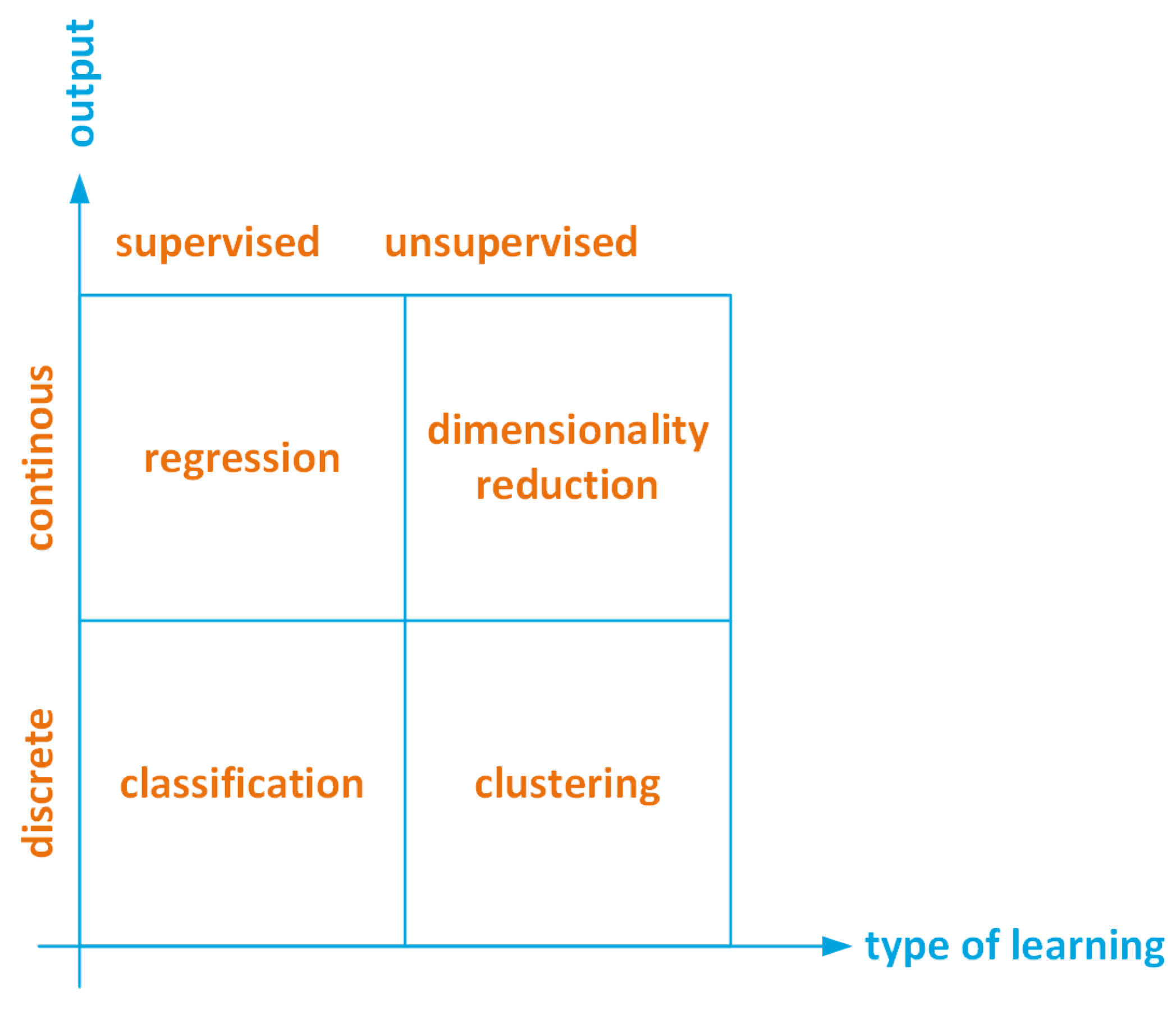
Figure 3, summarizes the four major classes of ML algorithms. The algorithms are classified according the type of output (either continuous or discrete) and the type of learning (either supervised or unsupervised).

2.3. Semi-Supervised Learning

Semi-supervised learning algorithms [33] are a class of algorithms able to learn from a partially labelled dataset. This approach is particularly beneficial when manipulating large datasets, since labelling is an expensive operation. Semi-supervised algorithms can be used when it is necessary to categorize large amounts of data, relying only on a few labelled examples. Typical applications include object segmentation, similarity detection and automatic labelling.

2.4. Reinforcement Learning

Reinforcement learning algorithms [34,35] rely on a decision-making agent that supervises the learning process. The learning algorithm samples the environment state (i.e., a vector of unlabelled features) and makes a decision according to the sampled data in a trial-and-error fashion. The decision leads to an action, and to a reward from the environment. The better the action, the higher the reward. The action to take is decided by a policy function f ( x i ) of the feature vector x i . The policy function is a mapping from R k to a finite set of actions A = { a 1 , a 2 , , a m } , namely
f ( x i ) : x i R k A .
The reinforcement learning algorithm can either be model-based [36,37] or model-free [38]. Model-free algorithms are more popular at present, as they are easier to implement and able to converge faster to an optimal solution for large-scale Markov Decision Processes (MDPs).

2.5. Machine Learning for IoT

IoT technology can leverage machine learning algorithms as the enabling technology for a wide number of applications [15,39,40,41,42,43]. The choice of the right machine learning (ML) algorithm basically depends on the use one wants to make of the collected data, and on the design requirements in terms of accuracy, linearity, number of parameters and hyperparameters, number of features and training time. These requirements can be even more stringent if the algorithm is supposed to run in hardware-constrained embedded devices or smart objects.
ML algorithms are often categorized either by learning style (supervised, unsupervised, etc.) or by similarities (regression algorithms, instance-based algorithms, regularization algorithms, etc.); however, in the context of IoT, a classification based on the application domain and the ML technique used can help to gain a much deeper insight into ML learning’s role in the IoT echosystem as an empowering technology.
Table 1 categorizes several ML algorithms that are suitable for execution on embedded devices according to their application domain and the ML technique (i.e., classification, prediction or learning agent). This classification does not pretend to be exhaustive and for more comprehensive treatment, the interested reader may refer to [43,44,45]. In particular, Ref. [45] is a comprehensive survey that explores the applications of ML algorithms to the whole IoT stack, including Cloud and Edge layers. To date, ML algorithms have mainly been used in the IoT device context for classification, prediction and device management purposes. Classification and prediction tasks rely, almost exclusively, on supervised and deep learning algorithms, whereas device management tasks rely on reinforcement learning techniques (both model-free and model-based). The supervised algorithms used more at the device level are: Support Vector Machine (SVM), K-Nearest Neighbour (KNN), Decision Tree (DT), Naive Bayes (NB), Hierarchical Mixture of Naive Bayes (HMNB), Regression Tree (RT) and Multiple Linear Regression (MLR). Unsupervised techniques such as Hidden Markov Model (HMM) and K-Means have also been reported, as well as ensemble learning techniques such as Random Forest (RF).
The deep learning techniques used in the IoT devices rely on Artificial Neural Networks (ANN) and Recurrent Neural Networks (RNN). Finally, the reinforcement learning techniques rely on Q-learning [38], Upper Confidence Bound (UCB) [61], Post-Decision State (PDS) [62], and Dyna [36,37].
ANNs can also be used to improve the quality of a prediction by tackling the problem of missing data. Techniques based on General Regression Neural Network (GRNN) networks and Successive Geometric Transformation Models (SGTM) [63,64] have been proven to be be very effective when dealing with the missing data problem.
The data collected can be used to predict a value or an outcome, to choose between two or more categories, to classify data or images, to analyse a text, to generate recommendations or find unusual occurrences such as in fraud detection, and to analyse and discover data structure. However, regardless of the target application, a trade-off must be found among the design constraints in order to match the expected results. Key requirements for ML models are reviewed in Appendix B.

3. Software Architecture

Machine learning is a very active field of research in both industrial and academic environments; consequently, there is a plethora of tools and libraries for ML and deep learning available [65]. However, all of them have been designed to manage huge amounts of data and rely on expensive hardware infrastructure to reduce the computation time by either increasing the parallelism (using, for example, computational models based on MapReduce [66]) or using GPUs as hardware accelerators.
The number of interconnected smart devices in the new IoT paradigm is increasing rapidly and there is a serious risk of saturating the network connection with the traffic between smart objects and the cloud infrastructure that has to process and analyse the sensed data. Consequently, part of the computational complexity must be shifted from cloud-to-edge infrastructure and end devices disclosing the path to a new computational paradigm for IoT. In the new computational model envisaged, raw data processing is mainly performed locally and in a hierarchical fashion from device to cloud, offloading the computation to the next level only when necessary [24,67]. However, to the authors’ knowledge, too little effort has been made to develop ML frameworks suitable for embedded devices to date.
Solutions based on Tensorflow lite are still not fully implementable in resource-constrained embedded devices [24]. In addition, Tensorflow lite is not a framework but a runtime environment that allows the running of pre-trained deep-learning models on mobile devices and microcontroller boards; thus, it lacks the flexibility of a full-fledged development framework and forces the programmers to develop applications only in Python or C/C++.
In recent years, Node.js has become a de facto industrial standard for the development of real-time distributed embedded systems and IoT applications [68,69,70,71] due to its suitability for running in embedded devices, its ability to implement both server and client applications, its low memory footprint and its asynchronous nature, which all make it very appealing for real-time applications. Despite all these advantages, there is still a widespread misconception that JavaScript (and hence Node.js) is not suitable for computation-intensive applications such as machine and deep learning, and Python is still the preferred language. Tensorflow.js (https://www.tensorflow.org/js (accessed on 10 February 2021)) is a first attempt to provide the JavaScript programming community with an industrial-proof tool to develop ML-based applications in JavaScript. Nonetheless, Tensorflow.js suffers the same limitations as its Python counterpart; namely, it is not a framework targeted towards embedded and resource constrained devices.
The dominant position of Node.js and JavaScript in the IoT panorama, and the necessity of shifting the computation from cloud to edge devices requires the development of a lightweight JavaScript ML framework that is able to run on embedded devices.
This section comprehensively targets the requirements and the architecture of such a framework. The rest of this section is devoted to the description of all the modules that form and integrate into the ML engine.

3.1. Overall Architecture

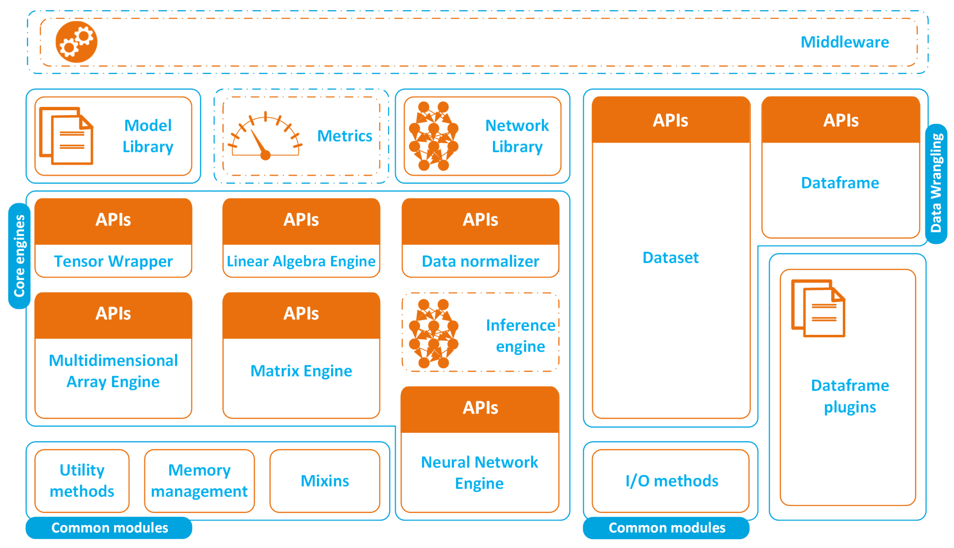
Figure 4 depicts the architecture of the ML framework described in this work. The software comprises several independent modules that expose Application Programming Interfaces (APIs). The core engine implements methods to manipulate multidimensional arrays, tensors and matrices, as well as first- and second-order Artificial Neural Networks [72].
The framework also provides a small library of common ML algorithms and a neural network. This library is an abstraction layer that sits on top of the core engines and provides the programmer with an abstraction layer that allows the development of applications without directly accessing the core APIs.
A typical ML pipeline, like the one depicted in Figure 2, also includes a data preparation step prior to the execution of the machine learning algorithm. Data preparation comprises several tasks that have to be performed on raw data in order to extract meaningful information. These include data normalization, data structuring and data aggregation. The framework provides APIs to manage datasets (basically, import and export data) and to manipulate data in tabular form through the Dataframe module.

3.2. Multidimensional Array Engine

The multidimensional array engine is inspired by the NumPy package and provides primitives to efficiently manipulate large multidimensional arrays of any size. The engine provides getter and setter methods as well as methods for array slicing. In order to maximise the efficiency and the flexibility of the implementation, the engine has been built on top of JavaScript typed arrays. Typed arrays provide high-level views on top of a binary raw-data buffer of fixed size, and allow JavaScript to manage data in multiple integer (both signed and unsigned) and floating point (both single- and double-precision) formats, as depicted in Figure 5.
A multidimensional array of k dimensions is characterised by its shape s = ( s 0 , s 1 , , s k 1 ) ; namely, a t-uple with the number of array elements along a given axis (or dimension). More specifically, s j (with j Z 0 + and s j N ) represents the number of elements along the axis j.
Array data are stored internally in row major format. The smaller indices represent the higher dimensions; thus, referring to the previous array shape definition, the pair ( s k 2 , s k 1 ) represents, respectively, the number of rows and columns of a matrix.
The engine performs a mapping f from a multidimensional array with a given shape s = ( s 0 , s 1 , , s k 1 ) to a one-dimensional strided array, namely
f : A i 0 , i 1 , , i k 1 R s 0 × s 1 × × s k 1 A j R n
where 0 i m s m 1 (with 0 m k 1 ) and 0 j n 1 = s 0 × s 1 × × s k 1 1 . In other words, the multidimensional array and its 1-D mapping have different shapes but the same number of elements.
The stride property is a t-uple s = ( s 0 , s 1 , , s k 1 ) that shows how many elements must be skipped in memory to move to the next position when traversing the array. The number of bytes to move in memory is automatically inferred by the engine from the stride and the type of array.
The index j of the mapping described by Equation (4), is a function g ( . ) of the stride s , the indices i 0 , i 1 , , i k 1 of the element of the multidimensional array, and of an offset x that denotes the position of the first element of the array within the ArrayBuffer data structure, namely
j = g ( s 0 , s 1 , , s k 1 , i 0 , i 1 , , i k 1 , x ) = x + m = 0 k 1 ( s m × i m )
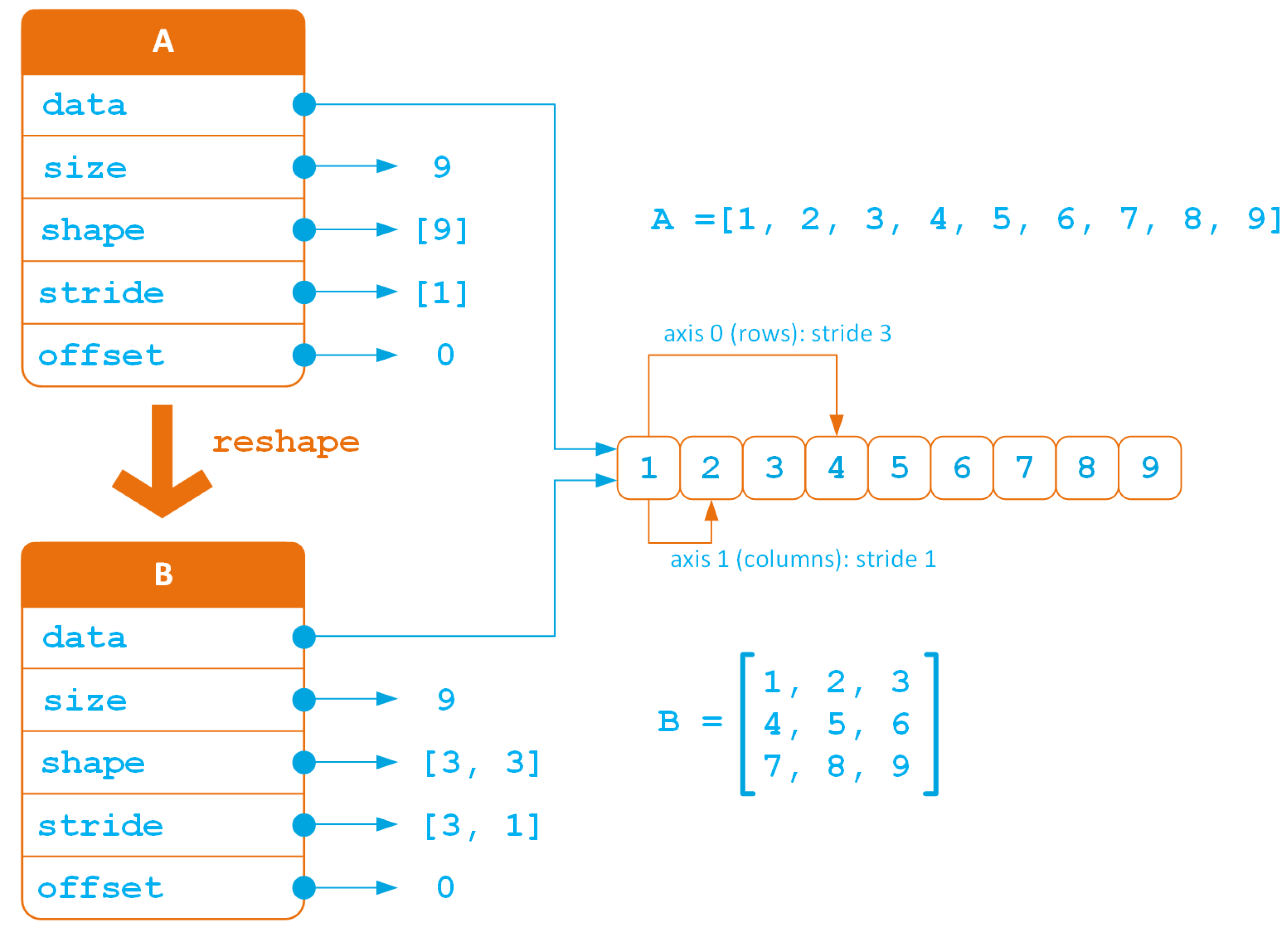
Defining an array through its shape, stride and offset leads to a more efficient internal representation, in which every transformation carried out on a given array A does not imply either duplication or reordering of the array elements, as shown in Figure 6, in the case of a reshape operation.
The reshape operation depicted in Figure 6 transforms a 1D array of nine elements into a three-by-three matrix. This operation implies a recomputation of the array strides. Observing that sizes and strides are given as number of array items, the engine automatically translates them into the right number of bytes according to the type of array element.
The multidimensional array engine allows for the represention of tensors with rank ρ 1 . In order to also represent scalar types (i.e., rank 0 tensors), the core engine is wrapped into a Tensor class that also provides a rich set of APIs to perform arithmetic operations on tensors. The Tensor Wrapper is compatible at API level with Tensorflow.js engine; thus, an application relying on the Tensorflow.js engine can be ported to our framework with very little effort, considering some slight differences that exist between the two frameworks. Table 2 summarises the API compatibility with Tensorflow.js. The implemented subset limits the compatibility only to ML learning algorithms, since Tensorflow.js wrappers for deep learning APIs relying on neural networks are still under development. In order to ensure software compatibility, coherent data types must be used. The multidimensional array engine supports all the JavaScript typed arrays (8, 16, 32 and 64 bits), whereas the Tensor wrapper also adds support to multidimensional arrays of Booleans and Strings. Conversely, Tensorflow.js only supports 32 bit data types, complex numbers encoded over 64 bit, Booleans and Strings.
Finally, the framework also supports broadcasting. Broadcasting consists of applying a given function to multidimensional arrays of different shapes, provided the shapes are compatible. For example, broadcasting allows for the addition of a multidimensional array to a scalar: the sum operation is broadcasted to all the individual elements of the array, adding them to the scalar term.
The multidimensional array engine is the core module used to build an ML model library, as depicted in Figure 4. The model library implements a set of prediction and classification algorithms that have been proven to be effective for IoT applications, as reported in Table 1. Table 3 reports the classification and prediction algorithms that were implemented in the framework model library.

3.3. Linear Algebra Engine

Linear algebra is intensively used in machine learning [73] when working with datasets and data preparation (for example, for  hot encoding and dimensionality reduction). Linear algebra is also used, for example, to solve linear regression problems and in Principal Component Analysis (PCA). Principal Component Analysis is an analysis method of multidimensional datasets that, generally, simplifies data analysis by projecting the high-dimensional data space onto a two-dimensional plane using the first two principal components. When the first two components fail to capture enough data variance, a 3D representation using the first three principal components should be considered in order to avoid loosing information. The structure of the projected data depends on the projection axis. Finding the information associated with a given projection is an eigenvalue problem. The eigenvectors of the covariance matrix represent the principal components, whereas the corresponding eigenvalues give an estimation of how much information is contained in each individual component. For this reason, the ML framework presented in this work also includes a set of advanced linear algebra features that can be used for data analysis and manipulation.
The Linear Algebra Engine (LAE) has been built on top of a Matrix Engine that provides all the basic matrix manipulation features (matrix transposition, basic matrix, rows and columns operations, Kroneker product, fast multiplication of large matrices using the Volker–Strassen algorithm, etc.) using the algorithms described in [73]. More specifically, the LAE implements the following features:
  • Eigenvalue decomposition (EVD);
  • LU decomposition;
  • QR decomposition;
  • Singular value decomposition (SVD);
  • Cholesky decomposition;
  • NIPALS algorithm;
  • Pseudo-inverse matrix computation;
  • Covariance matrix computation;
  • Determinant computation;
  • Linear dependencies computation.
Eigenvalue decomposition, a Nonlinear Iterative PArtial, Least Squares (NIPALS) algorithm [74] and a covariance matrix are used in machine learning for Principal Component Analysis. LU decomposition can be used to solve linear systems, compute determinants, invert a matrix and find a basis set of a vector space (i.e., finding linear independent rows of a matrix). The pseudo-inverse matrix can be used to compute a least-squares solution of a linear system.
Singular Value Decomposition (SVD) is a technique that is extensively used in machine learning and statistics for feature engineering, outlier detection, dimensionality reduction and noise removal. Cholesky decomposition is a special case of decomposition that can be applied to a symmetric and positive-definite matrix.

3.4. Artificial Neural Network Engine

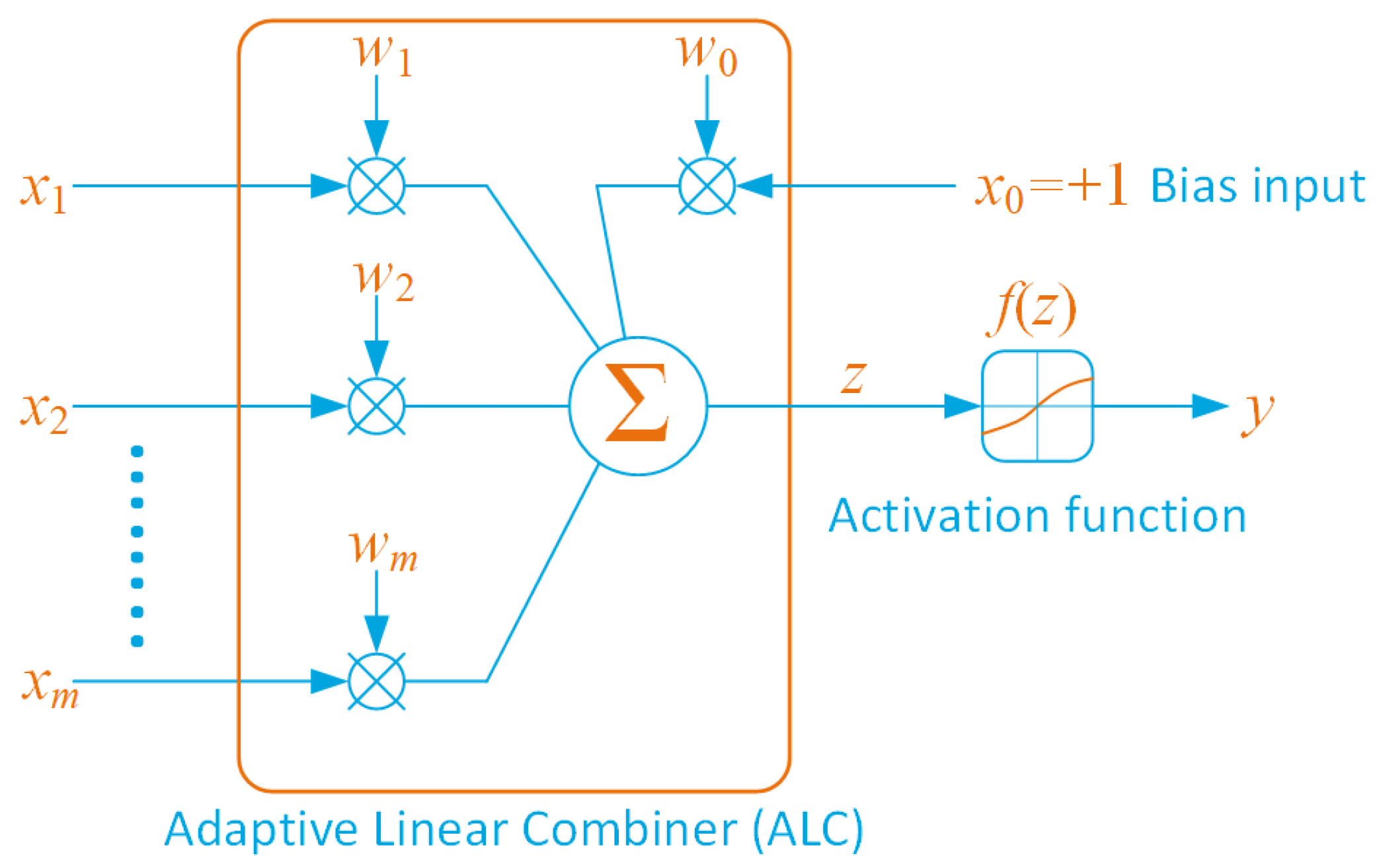
The Artificial Neural Network (ANN) engine, provides primitives to connect neurons in order to implement first- and second-order networks [72]. A Neural Network [75,76] is a collection of interconnected simple processing units, the neurons. The processing ability of the network lies in the weights associated to the neurons’ interconnections. The weights are obtained from a process of adaptation or learning in which the network is trained using specific data patterns. Figure 7 schematically depicts the operations performed by a neuron.
A neuron, i, of the network is formed by an Adaptive Linear Combiner (ALC) and by an activation function (or squashing function). The ALC performs the the sum of the weighted inputs x i j , namely
z i = b i + w i T x i
where
w i = ( w i 1 , , w i m ) x i = ( x i 1 , , x i m )
with b i = w i 0 being the bias and w i j being the weight of the j-th input of the i-th neuron of the network. The activation function f ( z ) is a function of the neuron activation potentialz and performs an output normalisation by returning a value y [ 0 , 1 ] . Several activation functions are available [77,78]; however, the ANN engine only implements the small subset reported in Table 4 that comprises both threshold, linear and non-linear activation functions.
The neural network learning process is implemented by combining gradient descent and backpropagation algorithms, as described in [76], on a training dataset whose true outcomes are known.
Several neural network topologies have been developed to date [79,80]; some of them have been implemented in the ANN engine and are available as library components that expose a simple API which provides primitives for creating and training the network. The following subsections briefly review the implemented networks.

3.4.1. Perceptron

The perceptron is a linear binary classifier that implements the neuron depicted in Figure 7. Since it is used for binary classification, the activation function f ( z ) is a simple hard limiter; thus, for a vector x R k of inputs, the results are
f ( x ) = 1 , if w · x + b > 0 0 , otherwise
where w is the vector of weights and w · x = i = 1 k w i x i is the dot product. The bias b is used to shift the decision boundary away from the origin and does not depend on the input values.

3.4.2. Long Short-Term Memory Network

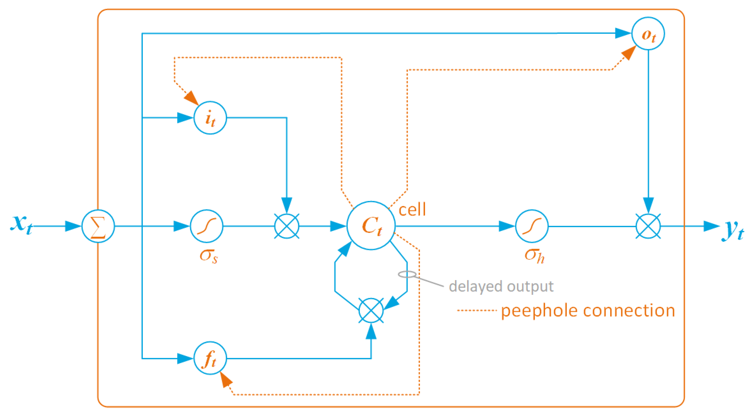
Long short-term memory (LSTM) is an artificial recurrent neural network (RNN) architecture, suitable for performing regression and classification based on a time series. It deals with the vanishing gradient problem (namely, an excessively low gradient that can prevent weights from changing during the training process and that, in the worst case, can completely stop the network training) that can occur when training recurrent neural networks. Several variants have been proposed [81]; however, the framework implements the most commonly used set-up, depicted in Figure 8.
In its basic implementation, the LSTM is formed by three gates (the input gate i t , the forget gate f t , and the output gate o t ), a block input activation function σ s , an output activation function σ h and a single cell C t (the Constant Error Carousel (CEC)). Function σ s is a sigmoid, whereas σ h is usually a hyperbolic tangent. Moreover, cell C t has a hyperbolic tangent activation function denoted with σ c .
Subindex t denotes the time-step. At  t = 0 , the initial cell values are C 0 = 0 and y 0 = 0 , respectively. Referring to Figure 8, x t R n is the input vector, C t R m is the cell state vector, i t R m the input gate activation vector, f t R m the forget gate activation vector, and  o t R m the output gate activation vector.
The LSTM network implements the following functions:
f t = σ s ( W f x t + W f p C t 1 + b f ) i t = σ s ( W i x t + W i p C t 1 + b i ) o t = σ s ( W o x t + W o p C t 1 + b o ) C t = f t × C t 1 + i t × σ c ( W c x t + b c ) y t = o t × σ h ( C t )
where W R m × n is the weight matrix for the CEC, input, forget and output cells; W p R m × m is the weight matrix for the peephole connections of the input, forget and output cells. Vector b R m is the bias vector of the CEC, input, forget and output cells. Finally, operator × denotes matrix element-wise multiplication (i.e., the Hadamard product).

3.5. Data Frame and Data Wrangling

The framework presented in this work also provides APIs for data acquisition, exploration, cleaning and manipulation, as depicted in Figure 4. Data wrangling is essential to transform raw data into a format that can be processed more efficiently by the machine learning engine.
The framework allows for the importation and exportation of large data files in several text formats (namely, CSV, TSV, PSV, JSON) and mapping the data onto a dataframe. A dataframe is a simple, two-dimensional schema of heterogeneous data with labelled axes. Primitives are available to manipulate rows and columns of a dataframe, which include filtering, selection, and joining. The core functionalities can be easily extended through a plugin system. Plugins that allow for the performance of statistical and matrix operations on a dataframe are available. Table 5 summarises the core features implemented by the data-wrangling engine of the framework.

4. Hardware Platforms and Framework Performance

A plethora of embedded computing platforms are available on the market [82,83]. Some new high-end embedded boards, such as Google Coral and NVIDIA Jetson Nano, also offer GPU acceleration. However, while an embedded GPU may be appealing for the acceleration of many machine learning algorithms, the increased cost of these platforms is a potential barrier for their adoption in many IoT applications, where the design is mainly cost-driven. In addition, server-side JavaScript GPU support is still at a very early stage, which limits the adoption of these boards for only Python and C/C++ applications.
Among all the boards available on the market, Raspberry Pis are the ones that probably offer the best trade-off between cost and performance. For this reason, the performance of the framework described in this work are stressed on a Raspberry Pi III (model B+) and a Raspberry Pi IV boards. Table 6 summarises the main features of the embedded computing boards used to evaluate the performance of the developed ML framework.
Observe that, although both boards rely on a 64-bit ARMv8 architecture, Raspberry Pi III B+ runs a 32-bit operating system (Raspbian v10), since it has only 1 GB memory and running a 64-bit operating system would not lead to any significant performance improvement. Conversely, in the proposed test set-up, Raspberry Pi IV runs a 64-bit operating system (Ubuntu 20.04).

4.1. Set-Up of the Benchmarking Environment

The performances of the embedded development boards have been stressed using a set of ad-hoc benchmarks to determine their suitability to run embedded machine learning algorithms. The main goal is stressing the performance of the underlying mathematical core rather than the execution speed of a ML algorithm; thus, the benchmarks are focused on analysing the performance of those operations that are more likely to be used in an ML algorithm.
The benchmark suite used to evaluate the performance of the ML framework runs on Node.js v14.4 and is formed of 29 typical operations applied to rank 1 and rank 2 tensors: vectors and matrices. Table 7 reports the operations that form the benchmark suite. Appendix C describes the architecture and the implementation of the benchmarking tool used to evaluate the performances of the ML framework in detail.

4.2. Performance Evaluation

Each benchmark operation is executed a variable number of times during a maximum timeframe of 5 s. The delay between consecutive test cycles is 5 ms, and the minimum number of samples measured during each cycle is 5. Test times and statistics are generated for each benchmark of the test suite. More specifically, the following timing metrics are calculated:
  • The time (in seconds) taken to complete the last cycle (cycle);
  • The elapsed time (in seconds) taken to complete the benchmark;
  • The time (in seconds) taken to execute a test once (period).
Moreover, the following test statistics are computed:
  • The number of samples acquired during the test;
  • The sample standard deviation σ ;
  • The sample variance σ 2 ;
  • The sample arithmetic mean m (i.e., the average execution time of the benchmark in seconds);
  • The standard error of the mean (SEM) computed as σ 2 n , where n denotes the number of samples;
  • The Margin of Error (MOE) computed over a confidence interval of 95%; namely, M O E γ = z γ × σ 2 n , where z γ denotes the quantile computed for a confidence level γ = 0.95 ;
  • The Relative Margin of Error (RME) expressed as percentage of the mean, namely, R M E = M O E γ m × 100 .
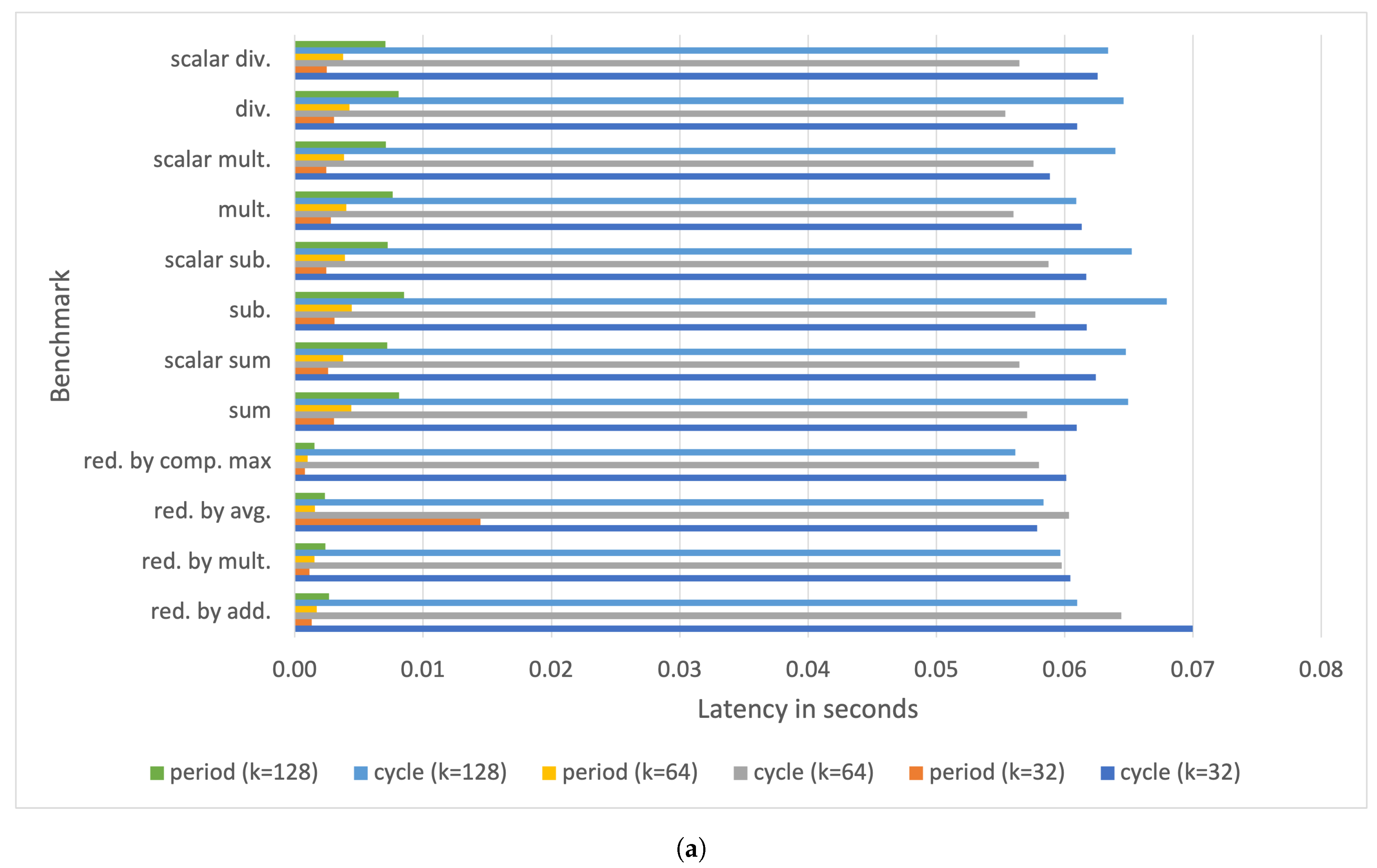
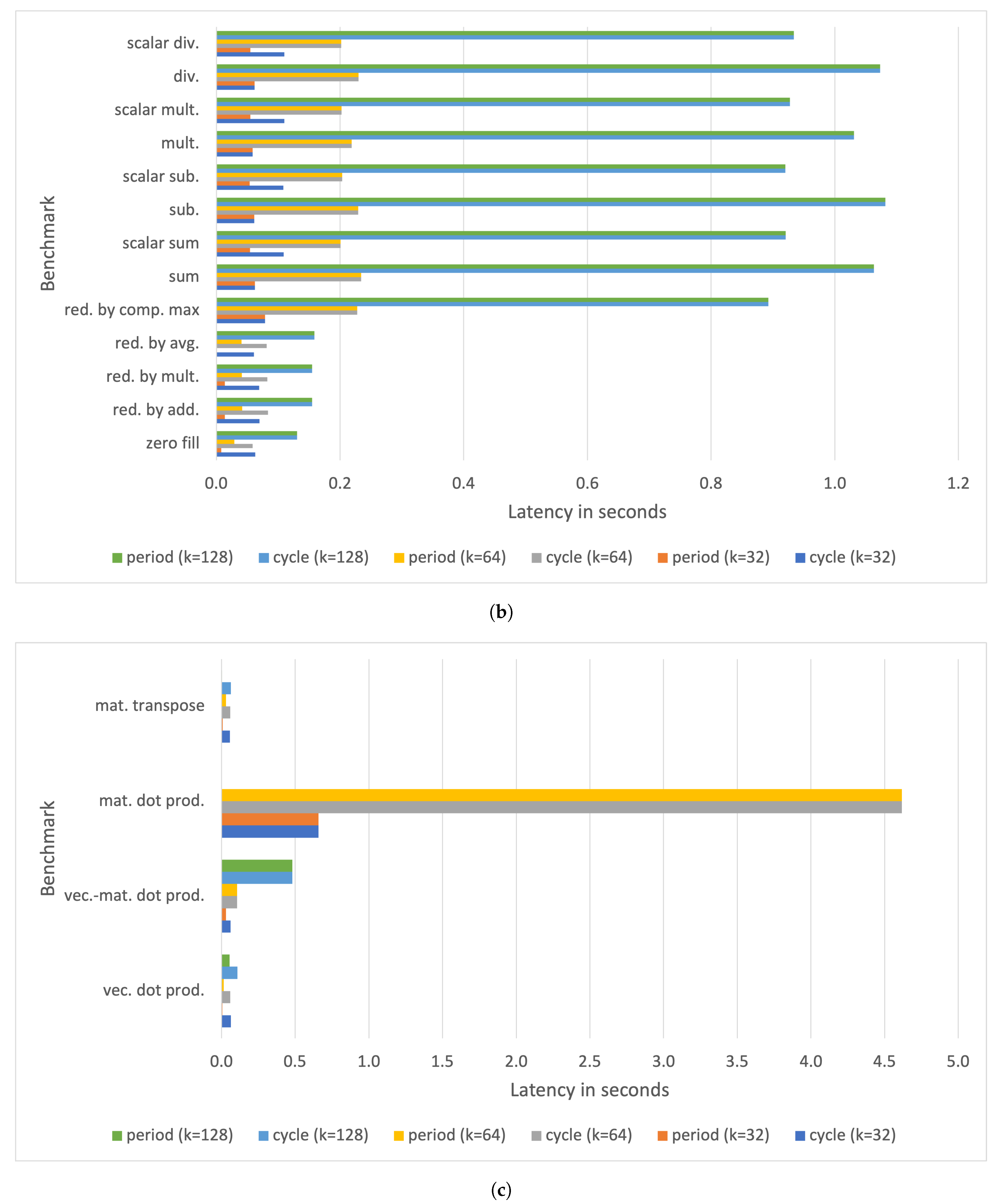
Performances have been evaluated for rank 1 tensors and vectors of dimension k and rank 2 tensors and matrices of dimension k × k , where k { 32 , 64 , 128 } . Figure 9 shows the cycle and period latencies for a Raspberry Pi III B+ board measured after running the benchmarking tool. The delay of rank 1 tensor operations ranges from few ms (for k = 32 ) to roughly 70 ms for (for k = 128 ). The latency increases to up 1.1  s for some rank 2 tensor operations (see Figure 9b).
The most time-consuming operation is the matrix dot product, whose latency exceeds 4.5  s for square matrices with k = 64 . Observe that the delay for a square matrix dot product with k = 128 is not reported since it exceeds 5 s, namely, the maximum time frame allocated for execution by the benchmarking tool.
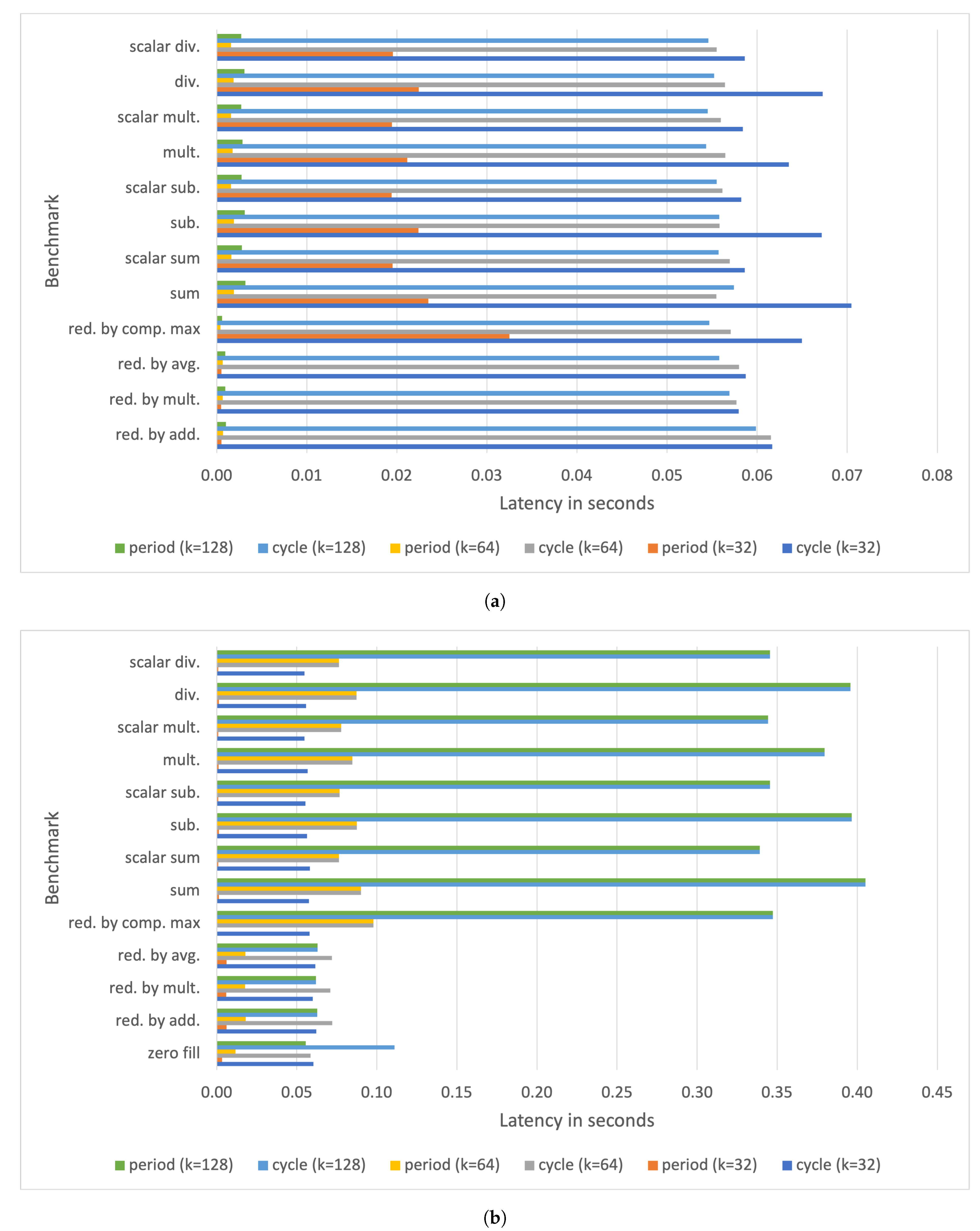
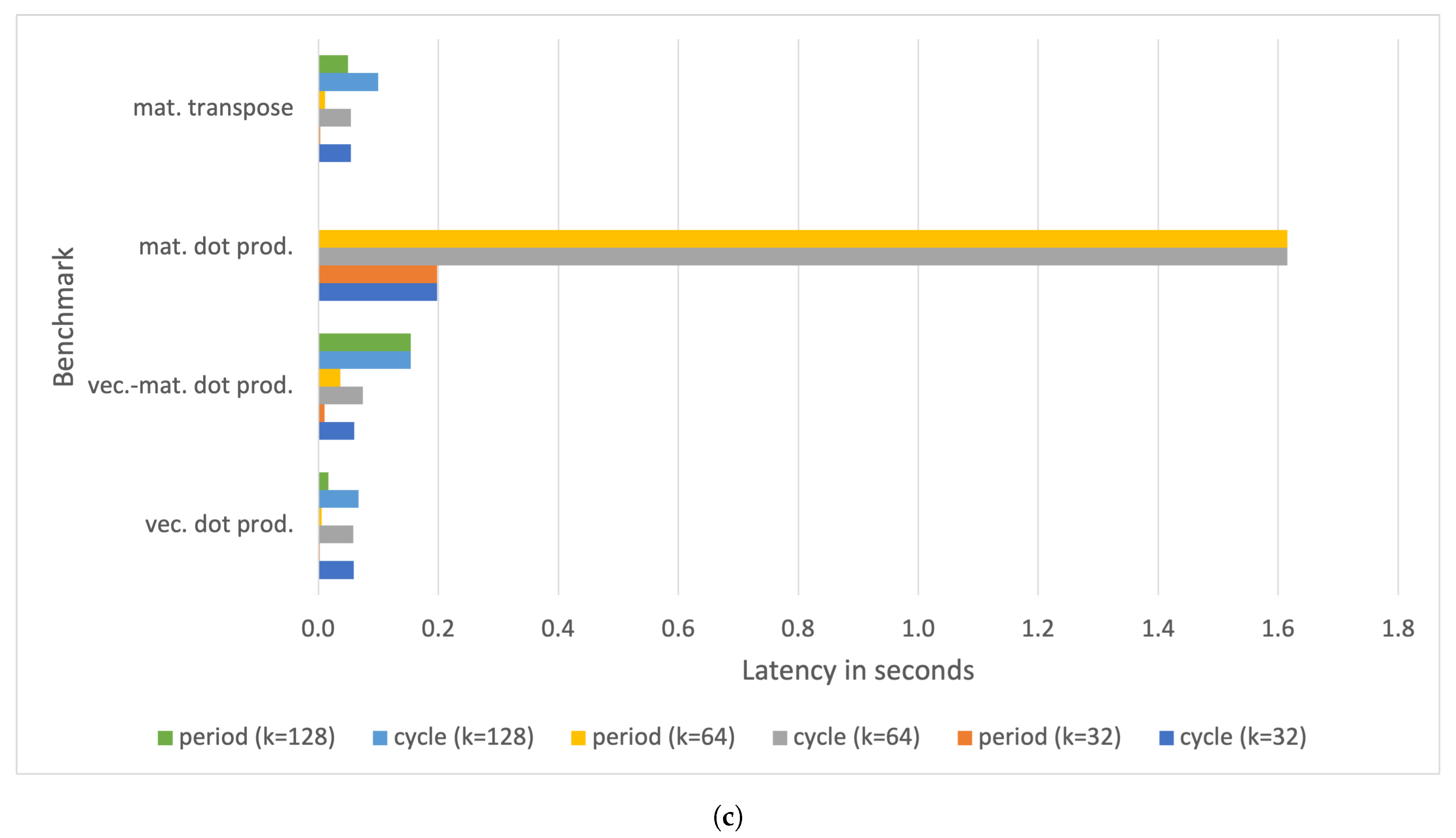
Figure 10 shows the cycle and period latencies for a Raspberry Pi IV board. Observe that for rank 1 tensor operations, the speedup with respect to the execution latencies measured for a Raspberry Pi III B+ board is roughly 2.
However, the improvement is even more significant for higher-order tensor and matrix operations, with speed-ups of up to 3.3 with respect to the benchmark execution times on a Raspberry Pi III B+. Nonetheless, for the Raspberry Pi IV, the latency of the square matrix dot product with k = 128 exceeds 5 s (the average delay is roughly 12.6  s), and it is not reported in the plots.

4.2.1. Summary of Raspberry Pi III measurements

Table 8, Table 9, Table 10, Table 11, Table 12, Table 13, Table 14, Table 15 and Table 16 report the detailed benchmark statistics for rank 1 and rank 2 tensor operations, and for vector and matrix operations.
Observe that the latency of matrix dot product for k = 128 is not reported, since it exceeds the maximum time allocated for the execution of a benchmark (namely, 5 s).
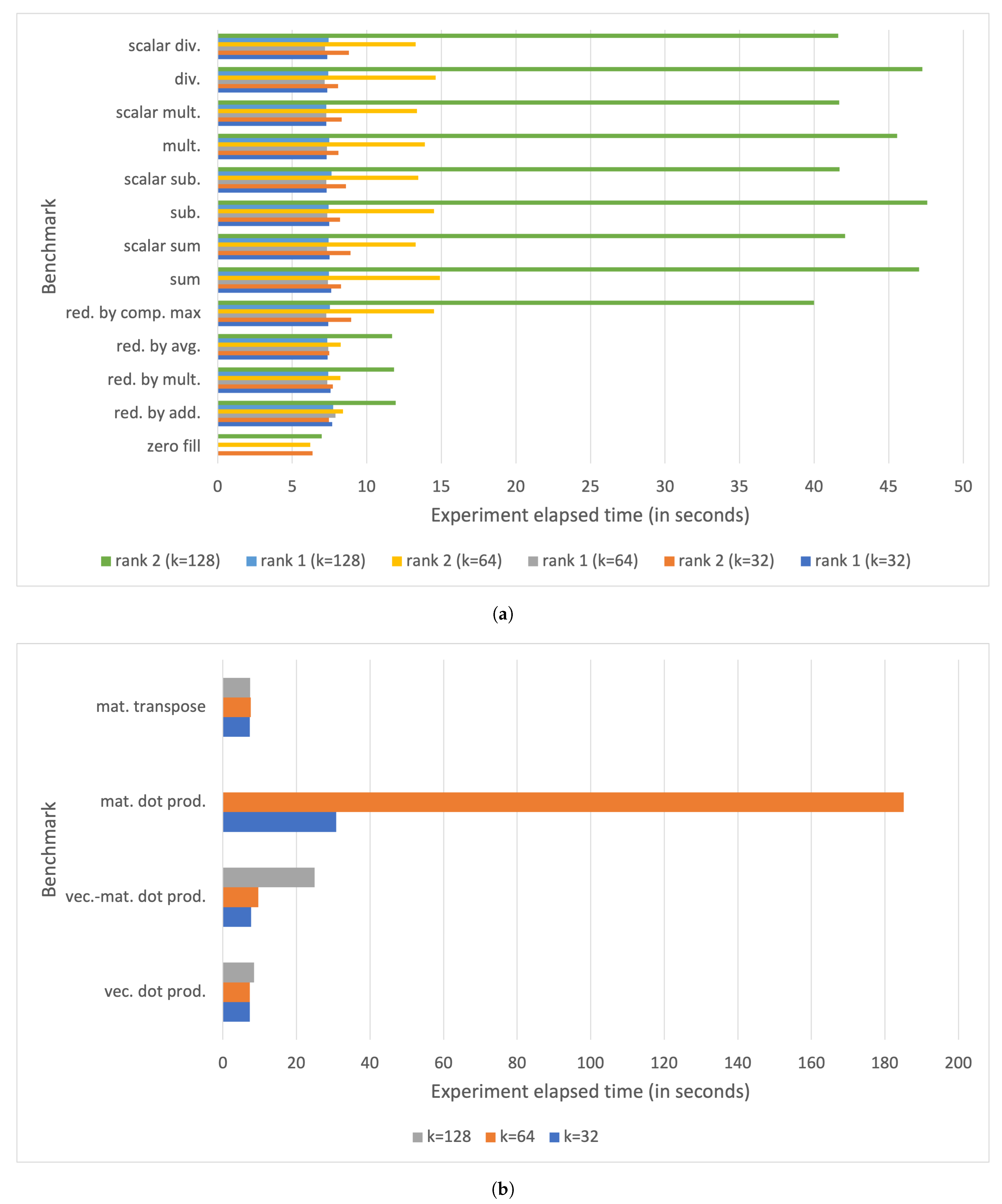
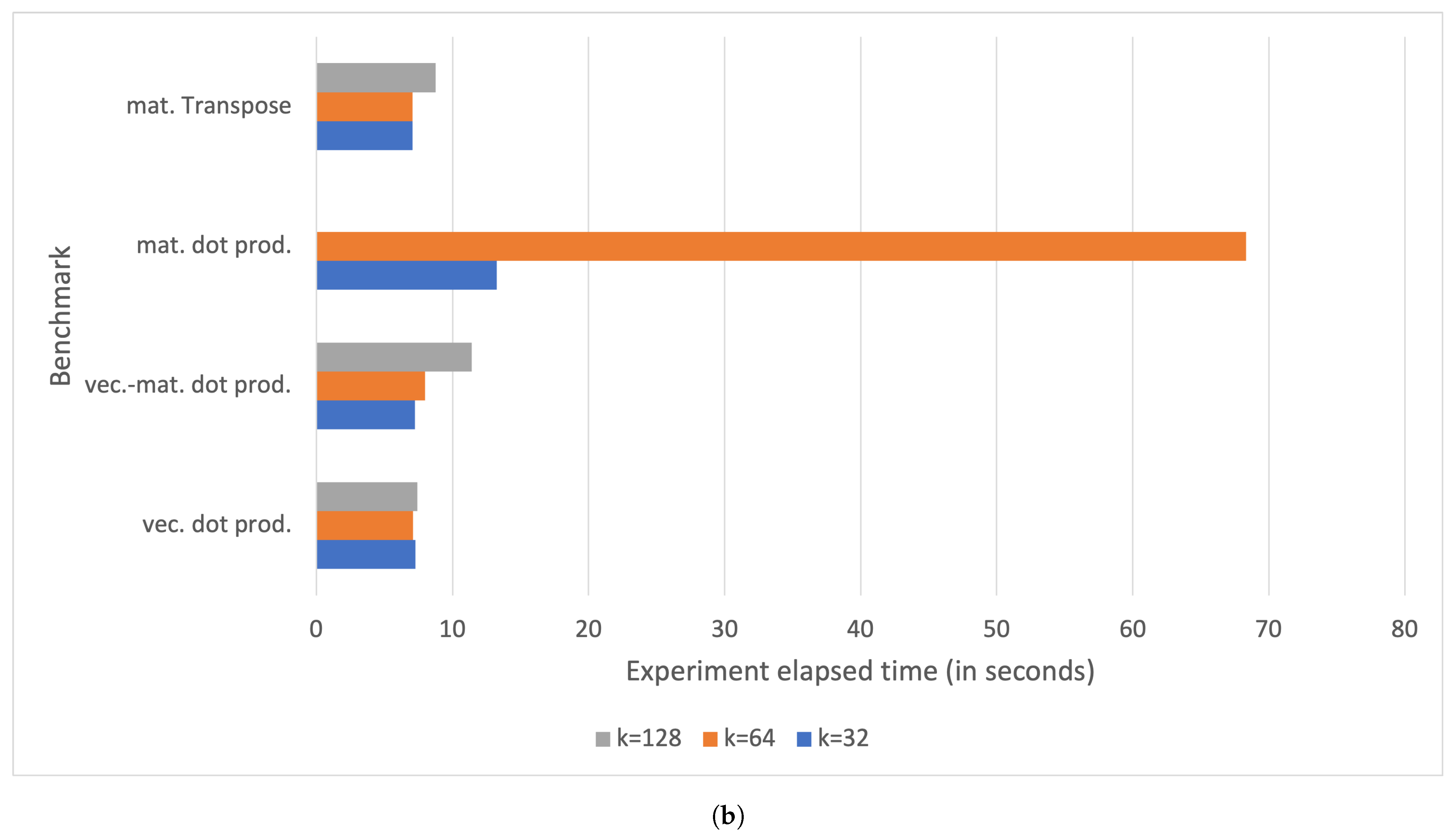
Finally, Figure 11 shows the elapsed times to compute the statistics for each benchmark on a Raspberry Pi III B+ board.
The overall time spent by the benchmarking tool performing all the measurements for a given benchmark ranges from a few seconds, in the case of rank 1 tensor operations with k = 32 , up to approximately 180 s, in the case of the square matrix dot product with k = 64 .

4.2.2. Summary of Raspberry Pi IV Measurements

Table 17, Table 18, Table 19, Table 20, Table 21, Table 22, Table 23, Table 24 and Table 25 report the detailed benchmark statistics for rank 1 and rank 2 tensor operations, and for vector and matrix operations executed on a Raspberry Pi IV embedded computer.
Observe that the latency of matrix dot product for k = 128 is not reported, since it exceeds the maximum time allocated for the execution of a benchmark (namely, 5 s).
Finally, Figure 12 shows the elapsed times to compute the statistics for each benchmark on a Raspberry Pi IV board. The overall time spent by the benchmarking tool to perform all the measurements for a given benchmark ranges from a few seconds, in the case of rank 1 tensor operations with k = 32 , up to approximately 68 s in the case of the square matrix dot product with k = 64 .

5. Discussion

In the previous section, the performance of a new ML framework targeted to IoT and embedded devices was stressed on Raspberry Pi III and IV boards. The collected results showed that these devices have enough computing power to perform tensor and matrix arithmetic with acceptable execution times for datasets of reasonable size (namely, up to 128 × 128 matrices of single-precision floating point numbers).
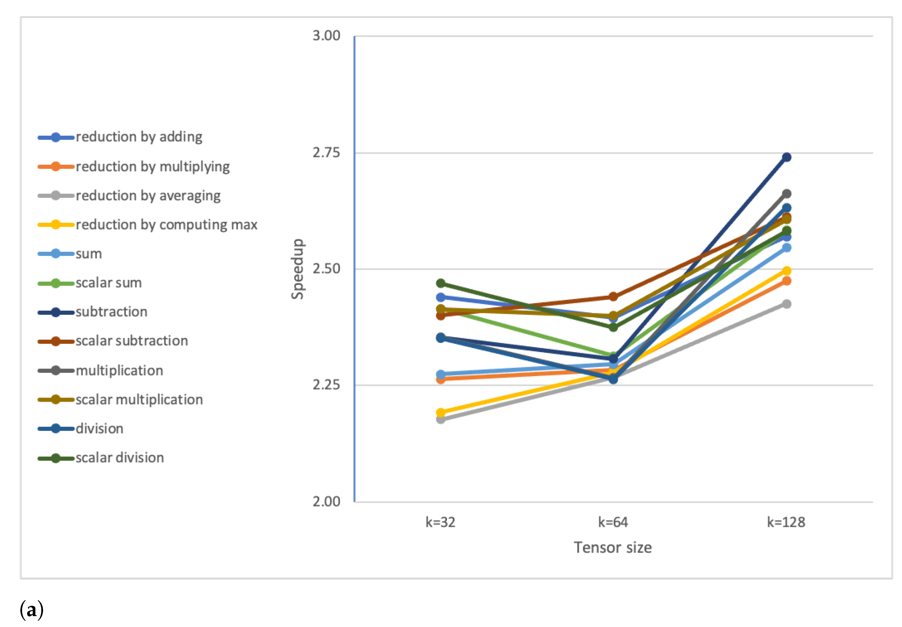
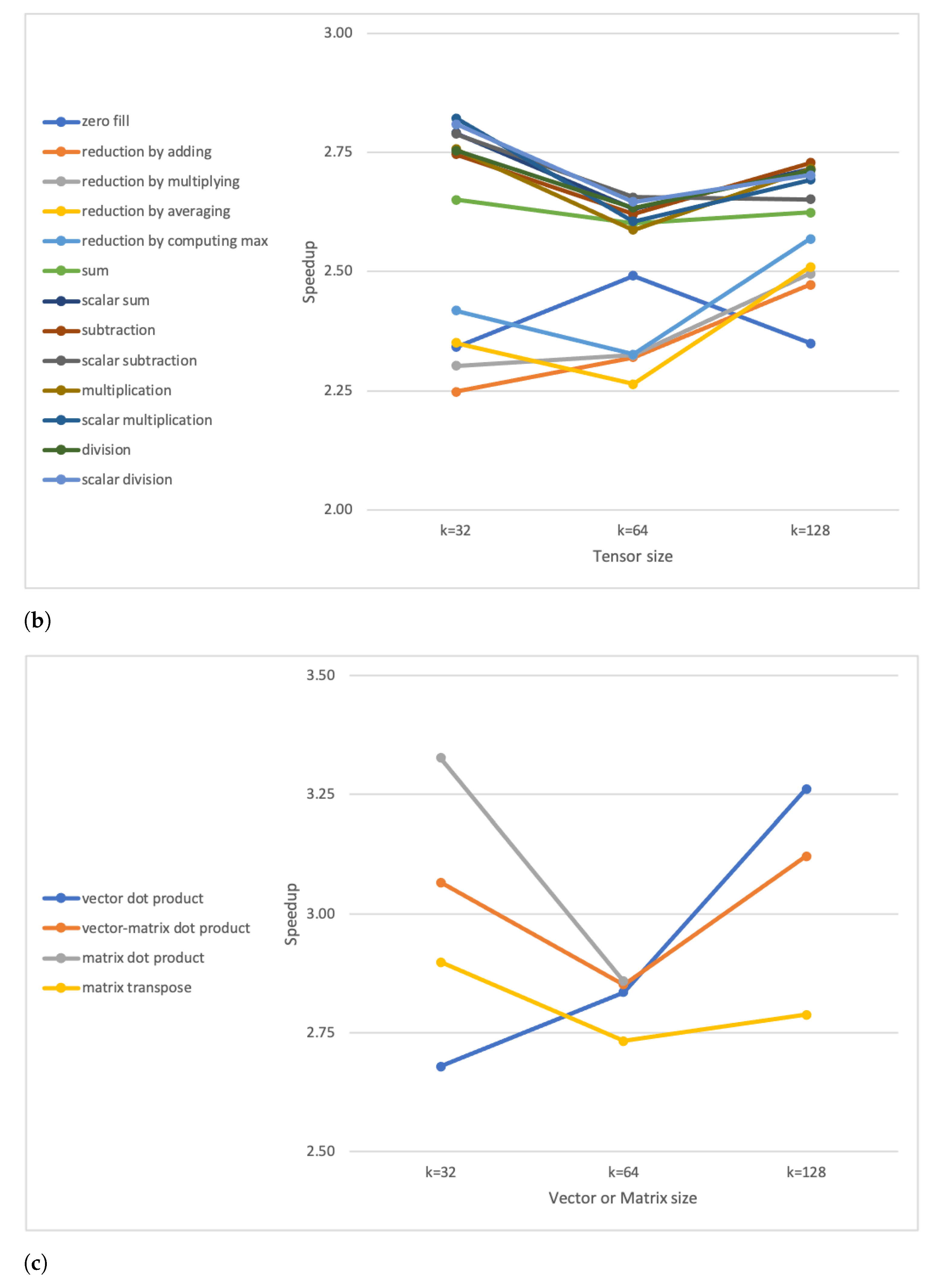
A substantial performance improvement was observed when executing the benchmark functions on a Raspberry Pi IV board, as also summarised in Figure 13.
The speed-ups were computed using the measured benchmark average execution values on Raspberry Pi III and IV boards for k { 32 , 64 , 128 } , with k being the size of either a tensor or an array or a k × k square matrix. The speed-ups, with respect to a Raspberry Pi III B+ board, were obtained by executing the framework on a Raspberry Pi IV ranging from roughly 2.2 to 3.3 . However, this improvement is exclusively due to the better hardware characteristics of the Raspberry Pi IV board, which is particularly suitable for computation- and memory-intensive operations.
Framework latency could be further decreased by optimising the code to increase the execution parallelism. Node.js is a single-threaded event-driven JavaScript runtime; however, by leveraging asynchronous constructions, it is possible to execute loop iterations in parallel as if they were executed by a multithreaded system.
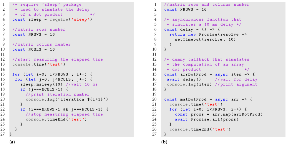
Consider the code snippets depicted in Listing 1. Snippet (a) simulates a matrix dot product using a synchronous programming style, whereas snippet (b) simulates the same operation using an asynchronous programming style with Promises.
Listing1. JavaScript code snippets that simulate a matrix dot product using (a) a synchronous programming, and (b) an asynchronous programming style.
Electronics 10 00600 i001
It is assumed that the code operates on 16 × 16 square matrices and that the array dot product has a delay of 10 ms. The execution latency is measured using the console.time() and console.timeEnd() function provided by the JavaScript console object.
After executing the two snippets on a Raspberry Pi III B+, the elapsed times are, respectively, 2.636  s for snippet (a) and 281.676  ms for snippet (b). Thus, writing code in an asynchronous fashion could lead to a theoretical speedup of 9.3 with respect to the sequential code. The performance increase is due to the fact that lines 23 and 24 of snippet (b) will run the arrDotProd task in parallel.
Refactoring the code in an asynchronous fashion by either “promisifying” the functions, as depicted in snippet (b) of Listing 1, or relying on third-party libraries, such as Async.js (https://caolan.github.io/async/v3/ (accessed on 10 February 2021)), is an appealing design choice since this will lead to a drastic reduction in the execution times measured reported in Section 4.
However, the framework mathematical core was designed and implemented according to the following main guidelines:
  • Implementation from scratch, without relying on any third-party package;
  • Use of a synchronous programming style for the core mathematical functions.
Implementing the core from scratch with zero dependencies avoids the code malfunctioning due to either broken dependencies or changes in the APIs of the third-party libraries. On the other hand, using a synchronous programming style, although detrimental from a performance perspective, could significantly ease the porting of the mathematical core to other programming languages.
The main limitation of languages based on garbage collection, such as Java, JavaScript or Python, is their lack of performance when compared to low-level languages such as C or C++. This is why well-established ML frameworks such as Tensorflow.js come with a core written in C/C++ in order to achieve high performances.
In the specific case of Node.js, the garbage collector relies on the Mark and Sweep algorithm [84]. Mark and Sweep solves the problem of cross referencing objects; however, it is relatively slow when compared to other garbage-collection algorithms such as Automatic Reference Counting (ARC), and this could be a problem when striving for better performance. A possible way to improve performance is writing a native Node.js module in C/C++ and provide JavaScript bindings. However, there is a better solution, which could potentially lead to much better results. In  recent years, Rust (https://www.rust-lang.org (accessed on 10 February 2021)) has attracted increasing attention from the programmer community. Rust is a low-level language designed for high speed, memory safety and thread safety, and it is particularly appealing for embedded applications. Rust does not rely on a garbage-collector, and memory management must be explicitly carried out by the programmer, as in C. However, unlike C, Rust relies on smart pointers, and the allocated memory is immediately released when a pointer falls out of scope. In addition, in most cases, Rust outperforms C and C++ [85] (especially when using concurrency and multithreading) and provides seamless integration with JavaScript and Node.js [86].
From this perspective, optimising JavaScript code makes no sense, since a much better performance can be achieved by porting computation- and memory-intensive operations to Rust and providing bindings for the JavaScript application. For this reason, the framework ML core is in the process of being ported to Rust. Combining the power and speed of Rust and the flexibility and the large ecosystem of Node.js has the potential to enable new ML applications in which part of the data analysis and processing is shifted to the embedded device itself.
The framework presented in this work is suitable for all those IoT applications that rely on batch-processing of the sampled data [87,88,89]; however, it is envisaged that the performance boost achievable by rewriting the mathematical core in Rust will make this framework suitable for that class of applications that requires stream and real-time processing.
A general-purpose and embeddable ML framework may potentially enable new architectures, in which some of the computational tasks are shifted to the edge devices. In such a context, the software presented in this work is now being tested in a staging environment for metabolomics applications [90]. Metabolomics requires batch processing of huge amounts of data; thus, the target requirements in terms of data-throughput perfectly match the framework current characteristics. The goals of this ongoing research are:
  • Automating the whole ML workflow, as depicted in Figure 2, by leveraging the data-wrangling features and the ML algorithms bundled with the framework;
  • Integrating data versioning systems such as DVC (https://dvc.org/ (accessed on 10 February 2021)) into the ML pipeline;
  • Stressing and analysing the performances of the classification algorithms which are more suitable for metabolomic problems;
  • Digitalising the existing metabolomics lab infrastructure, as envisaged in [91], using an evolution of the IoT architecture previously proposed in [9], in which each lab machine is provided with software wrappers that allow autonomous data analysis on the sampled data;
  • Leveraging the API-level compatibility with Tensorflow.js to implement load-balancing algorithms that seamlessly and dynamically shift ML algorithms’ execution from edge devices to edge servers running Tensorflow.js;
  • Deploying and stressing novel IoT architectures that rely on intra-lab sensor meshing and a distributed MapReduce with federated execution [92].
The framework also provides Artificial Neural Network (ANN) support; however, it suffers from the same limitations as other implementations, such as Tensorflow Lite, when dealing with Deep Neural Networks. Deep neural models are computationally and memory-expensive, and require a compilation step to simplify the network model and make it suitable for execution in a resource-constrained edge device. A possible way of simplifying Deep Neural Networks consists of using pruning algorithms to reduce the number of neurons and synapses [93]. As outlined in Section 3.1, the ANN inference engine is still under development, which limits the application field to algorithms that rely on shallow neural networks. This means, at this stage of development, that the framework cannot efficiently deal with some kinds of application, such as, for example, efficient power management in networked microgrids [94,95,96], since they require algorithms that can only be efficiently implemented using deep convolutional neural networks [97].

6. Conclusions

This work deals with the design and implementation of an ML learning framework suitable for embedded devices and IoT applications. The framework also provides APIs for artificial neural networks and data-wrangling and analysis. The following stages took place during the design process:
  • First, a set of ML algorithms suitable for IoT applications were identified through a careful literature review;
  • Then, the core supporting software infrastructure was developed, privileging, by design, portability to other programming languages;
  • Finally, the core infrastructure was stressed using an ad-hoc bechmarking tool in order to gain a better insight into the limitations imposed by the software architecture and the underlying hardware.
Although development is still at an early stage, the results are encouraging, and the measurements demonstrate that it is possible to embed a fully fledged ML framework into a resource-constrained computing board.
The framework was demonstrated on Raspberry Pi III and IV boards, and its performances were evaluated for several load conditions with rank 1 and rank 2 tensors and matrices and for several values of the dimension k. The delay in rank 1 tensor operations on a Raspberry Pi III board ranges from a few ms (for k = 32 ) to roughly 70 ms for (for k = 128 ). The latency increases to up to 1.1  s for some rank 2 tensor operations. The most time-consuming operation is the matrix dot product, measured for a k × k matrix with k = 64 , whose latency is approximately 4.5  s.
Matrix and tensor operations are both computation- and memory-intensive; thus, migrating to a Raspberry Pi IV board leads to a significant speed-up of up to 3.3 with respect to the performances measured for the Raspberry Pi III set up. Detailed measurements are reported in Table 8, Table 9, Table 10, Table 11, Table 12, Table 13, Table 14, Table 15, Table 16, Table 17, Table 18, Table 19, Table 20, Table 21 and Table 22.
The framework is suitable for all applications that rely on batch-data-processing and is now being tested in a set-up suitable for metabolomics applications, focusing on ML pipeline automation and algorithm performance and optimisation.
A further performance boost can be achieved by migrating the mathematical core to a high-performance language suitable for embedded applications like Rust, and implementing the bindings for Node.js to connect the new optimised core to the rest of the framework.
It must be highlighted that the proposed solution differs from other solutions, such as Tensorflow Lite. While the latter is a runtime environment that allows a pre-trained model to be run on a small device, the solution described in this work is a full-fledged and modular framework that offers the possibility of implementing the complete ML workflow onto an embedded device.
Hardware and software technologies are mature enough to allow the implementation of a lightweight, yet high-performance ML core, capable of running in embedded devices, thus offering a path to a new pervasive computing paradigm in which the IoT devices are not merely data collectors and forwarders, but real “smart” devices with enough computing power. In such a context, Node.js and Rust are really appealing technologies and seem to guarantee enough performance and flexibility to achieve this goal in the medium-term.
Author Contributions

Conceptualization, G.C. and A.T.; methodology, G.C. and A.T.; software, G.C.; validation, G.C. and A.T.; investigation, G.C. and A.T.; writing—original draft preparation, G.C.; writing—review and editing, G.C. and A.T.; supervision, A.T. All authors have read and agreed to the published version of the manuscript.

Funding

This research received no external funding

Conflicts of Interest

The authors declare no conflict of interest.

Abbreviations

   The following abbreviations are used in this manuscript:
AIArtificial Intelligence
ALCAdaptive Linear Combiner
ANNArtificial Neural Network
APIApplication Programming Interface
ARCAutomatic Reference Counting
BLEBlueTooth Low Emission
CECConstant Error Carousel
CoAPConstrained Application Protocol
CSVComma Separated Value
CPUCentral Processing Unit
DTDecision Tree
EVDEigenvalue Decomposition
GPIOGeneral Purpose Input Output
GPUGraphics Processing Units
HMMHidden Markov Model
HMNBHierarchical Mixture of Naive Bayes
IoTInternet of the Things
JSONJavaScript Object Notation
KNNK-Nearest Neighbour
LAELinear Algebra Engine
LSTMLong Short-Term Memory
LDDDRLow-Power Double Data Rate
LTSLong-Term Support
MDPMarkov Decision Process
MLMachine Learning
MLRMultiple Liner Regression
MOEMargin of Error
MQTTMessage Queue Telemetry Transport
NBNaive Bayes
NIPALSNonlinear Iterative PArtial Least Squares
OSOperating System
PCAPrincipal Component Analysis
PDSPost-Decision State
PSVPipe Separated Value
RAMRandom Access Memory
RNNRecurrent Neural Network
ReLURectified Linear Unit
RFRandom Forest
RMERelative Margin of Error
RTRegression Tree
SEMStandard Error of Mean
SDRAMSynchronous Dynamic RAM
SVDSingular Value Decimposition
SVMSupport Vector Machine
TSVTab Separated Value
UCBUpper Confidence Bound
USBUniversal Serial Bus
WiFiWireless Fidelity

Appendix A. Optimal Data Fitting

Overfitting and underfitting are causes of poor performance in machine learning models. More specifically:
  • Overfitting is related to a lack of generalization of the ML model due to a too-accurate training. Namely, the model is very specific and too fit for the training data, and fails when it is applied to data collected in the future, generating erroneous outcomes;
  • Underfitting happes when the learning model is not accurate enough to capture the relationship among new data. Namely, the model fails to learn the problem from the training dataset.
The approximation with a simple straight line of Figure A1a is not a good approximation because it does not render the nonlinear relationship between between the model variables x and y. This model is underfit to the data and it does not perform well, even with the training data. Conversely, the model of Figure A1c is an example of overfitting. This model learns all the details and noise of the training data; namely, the model captures the random fluctuations in the training data and incorporates them as part of the model. The problem is that irrelevant details and noise do not apply to new data and can negatively impact the model’s ability to generalise. Finally, Figure A1b depicts a model with optimal fit. Optimal fit lies between underfitting and overfitting. The optimal fit can be found by analysing the model’s behaviour for the training and test datasets. During the training process, the error on both training and test datasets decreases; however, when the model is overtrained, the error in the training dataset decreases (i.e., the model is overfitting), whereas the error in test dataset starts to increase. The optimal fit is the point just before the error on the test dataset starts increasing.
Figure A1. Different model approximations: (a) model with underfitting, (b) model with optimal fit, and (c) model with overfitting.
Electronics 10 00600 g0a1
Underfitting is not a problem, because it can be easily detected by selecting a good performance metric. Conversely, overfitting is a very common problem in nonparametric and nonlinear models, and can be tackled using resampling techniques or suitably tuning the model’s hyperparameters to limit or constrain the amount of details learned by the model.

Appendix B. Key Requirements for ML Models

Appendix B.1. Accuracy

In machine learning, accuracy is the measure of the effectiveness of an ML model in terms of correct predictions or classifications. Accuracy can be measured using classification accuracy. Classification accuracy (or simply Accuracy) is defined as the ratio of the number of correct predictions to the number of total predictions performed on the dataset, namely
Accuracy = number of correct predictions total number of predictions
However, relying only on this metric to evaluate the effectiveness of a ML algorithm could be misleading, especially in the case of heavily unbalanced datasets. This is not allowable in cases when the cost of a misclassification is high (e.g., not detecting a rare disease).
Several metrics can be used to suitably evaluate the performance of an ML algorithm; the interested reader may refer to [98,99] for a detailed treatment.

Appendix B.2. Training Time

In supervised learning, training time is the time spent training the ML model using historical data in order to build a model which minimises the prediction errors. The training time is strictly related to accuracy and to the type of ML algorithm used.

Appendix B.3. Linearity

A prediction function can be either linear or non-linear. Given a feature vector x i R k , a linear prediction function can be represented as
y ^ i = w 0 + j = 1 k w j · x i j
where x i j denotes a property of the of the feature vector x i , y ^ i is the predicted target (or label), and the coefficients w 0 , , w k are the parameters of the model. Examples of linear ML algorithms are linear regression, logistic regression, and support vector machine. Conversely, a non-linear ML algorithm is characterized by a non-linear prediction function. Examples of non-linear ML algorithms are naive Bayes, Gaussian naive Bayes, and  K-nearest neighbours.
Usually, linear algorithms are a good starting point, since they used to be algorithmically simpler and faster to train with respect their non-linear counterparts. However, they are not always the best choice, as shown in the examples of Figure A2.
Figure A2. Linear approximation of the prediction function for (a) a binary classifier with a non-linear boundary, and (b) a dataset with non-linear trend.
Electronics 10 00600 g0a2
In the case of Figure A2a, a linear approximation to classify the dataset would lead to low accuracy, since the class boundary is clearly non-linear. Analogously, as depicted in Figure A2b, a linear approximation of a dataset with a non-linear trend would result in large prediction errors.

Appendix B.4. Number of Parameters and Hyperparameters

The terms parameter and hyperparameter are sometimes used interchangeably in machine learning; however, they are not the same thing. If we refer to the simple regression model of Equation (A2), the coefficients w 0 , w 1 , w k represent the model parameters. Thus, parameters are properties of the training data that are not set manually but tcan be learned or estimated from data during model training. An ML model can be either parametric or nonparametric, depending on whether it has a fixed number of parameters. Examples of model parameters are the coefficients in a linear or logistic regression, or the weights in an artificial neural network. Conversely, a hyperparameter is a configuration external to the model that cannot be learnt from the data and must be set manually and properly tuned to a specific problem. Hyperparameters are necessary for the correct set-up of the estimation process of the learning parameters. Examples of model hyperparameters are the k of the K-nearest neighbour algorithm, C and σ for support vector machine algorithm, and the number and size of the hidden layers of a neural network.
The number of parameters and hyperparameters of an ML model determine the algorithm performance, since their training time is sensitive to their number.

Appendix B.5. Number of Features

A feature x i j x i ¯ is a measurable property or characteristic of the phenomenon under observation. A feature is the basic building block of a dataset. More specifically, one row of the dataset represents an observation or experiment x i ¯ , whereas each column of the dataset represents a feature. The number of features depends on the type of phenomenon observed; for example, genetic and textual data are characterized by a large number of features.
The performance of a machine-learning algorithm heavily depends on the number of features to be analysed, since this can make the training time extremely long.
The quality of a dataset can be improved with processes like feature selection and feature engineering. Feature selection is aimed at removing properties that are either redundant or not relevant from the dataset, without sacrificing the accuracy of the ML algorithm. The benefits of good feature selection are:
  • Reducing the chance of overfitting the model;
  • Reducing the ML algorithm training time;
  • Improving the model’s interpretability by highlighting only those properties that are more relevant to performing a good prediction.
Feature engineering is the process of combining an existing model’s features to create new ones that can provide a deeper understanding of the problem, improving the accuracy of the model and helping it to converge faster to an optimal solution.

Appendix C. Benchmarking Tool Architecture and Implementation

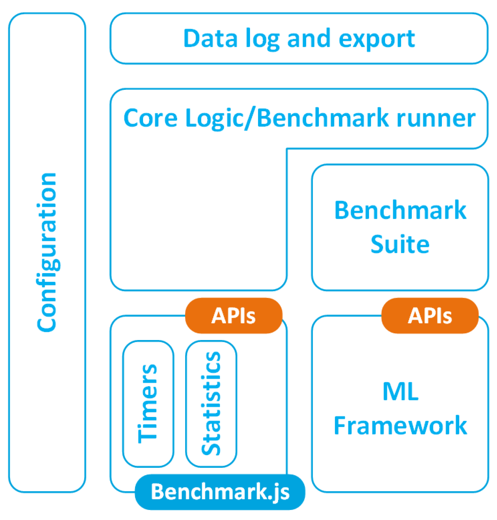
Figure A3 depicts the architecture of the benchmark tool used to evaluate the performances of the ML framework presented in this work. The tool used was built on top of the Benchmark.js (https://benchmarkjs.com (accessed on 10 February 2021)) library. This library provides low-level APIs, to control system timers and perform statistical operations on the measured data.
The benchmark tool comprises the following modules:
  • A benchmark suite; namely, a module that invokes the primitives of the ML framework that must be evaluated;
  • A benchmark runner, in charge of executing the measurements on both synchronous and asynchronous modules of the ML framework and collecting the measured data by leveraging the primitives provided by Benchmark.js;
  • A data log and export module in charge of logging results and preparing and formatting the data in several text-exporting formats (CSV, TSV, etc.) that are suitable for import into a spreadsheet;
  • A configuration module that parses a configuration file with the general benchmark set-up (number of simulations, duration, data output format, etc.) and configures all the benchmark modules accordingly.
Figure A3. Architecture of the benchmark tool.
Electronics 10 00600 g0a3

References

  1. Ahamed, F.; Farid, F. Applying Internet of Things and Machine-Learning for Personalized Healthcare: Issues and Challenges. In Proceedings of the 2018 International Conference on Machine Learning and Data Engineering (iCMLDE), Sydney, Australia, 3–7 December 2018; pp. 19–21. [Google Scholar]
  2. Sen, S.; Datta, L.; Mytra, S. (Eds.) Machine Learning and IoT: A Biological Perspective; CRC Press: Boca Raton, FL, USA, 2019; ISBN 978-1-13-849269-1. [Google Scholar]
  3. Walter, K.-D. AI-based sensor platforms for the IoT in smart cities. In Big Data Analytics for Cyber-Physical Systems. Machine Learning for the Internet of Things; Dartmann, G., Song, H., Schmeink, A., Eds.; Elsevier: Amsterdam, The Netherlands, 2019; pp. 145–166. ISBN 978-0-12-816637-6. [Google Scholar]
  4. Cornetta, G.; Touhafi, A.; Muntean, G.-M. (Eds.) Social, Legal, and Ethical Implications of IoT, Cloud, and Edge Computing Technologies; IGI Global: Hershey, PA, USA, 2020; ISBN 978-1-79-983817-3. [Google Scholar]
  5. Kumar Koditala, N.; Shekar Pandey, P. Water Quality Monitoring System Using IoT and Machine Learning. In Proceedings of the 2018 International Conference on Research in Intelligent and Computing in Engineering (RICE), San Salvador, El Salvador, 22–24 August 2018; pp. 1–5. [Google Scholar]
  6. Ullo, S.L.; Sinha, G.R. Advances in Smart Environment Monitoring Systems Using IoT and Sensors. Sensors 2020, 20, 3113. [Google Scholar] [CrossRef]
  7. Hossam, M.; Kamal, M.; Moawad, M.; Maher, M.; Salah, M.; Abady, Y.; Hesham, A.; Khattab, A. PLANTAE: An IoT-Based Predictive Platform for Precision Agriculture. In Proceedings of the 2018 International Japan-Africa Conference on Electronics, Communications and Computations (JAC-ECC), Alexandria, Egypt, 17–19 December 2018; pp. 87–90. [Google Scholar]
  8. Araby, A.A.; Abd Elhameed, M.M.; Magdy, N.M.; Said, L.A.; Abdelaal, N.; Abd Allah, Y.T.; Darweesh, M.S.; Fahim, M.A.; Mostafa, H. Smart IoT Monitoring System for Agriculture with Predictive Analysis. In Proceedings of the 2019 8th International Conference on Modern Circuits and Systems Technologies (MOCAST), Thessaloniki, Greece, 13–15 May 2019; pp. 1–4. [Google Scholar]
  9. Cornetta, G.; Touhafi, A.; Togou, M.A.; Muntean, G.-M. Fabrication-as-a-Service: A Web-Based Solution for STEM Education Using Internet of Things. IEEE Internet Things J. 2020, 7, 1519–1530. [Google Scholar] [CrossRef]
  10. Mathur, P. Machine Learning Applications Using Python Cases Studies from Healthcare, Retail, and Finance; Springer Science + Business Media: New York, NY, USA, 2019; ISBN 978-1-4842-3787-8. [Google Scholar]
  11. Ray, P.P. An Introduction to Dew Computing: Definition, Concept and Implications. IEEE Access 2018, 6, 723–737. [Google Scholar] [CrossRef]
  12. Reddy, R.R.; Mamatha, C.; Reddy, R.G. A Review on Machine Learning Trends, Application and Challenges in Internet of Things. In Proceedings of the 2018 International Conference on Advances in Computing, Communications and Informatics (ICACCI), Bangalore, India, 19–22 September 2018; pp. 2389–2397. [Google Scholar]
  13. Sharma, K.; Nandal, R. A Literature Study On Machine Learning Fusion with IOT. In Proceedings of the 2019 3rd International Conference on Trends in Electronics and Informatics (ICOEI), Tirunelveli, India, 23–25 April 2019; pp. 1440–1445. [Google Scholar]
  14. Zou, Z.; Jin, Y.; Nevalainen, P.; Huan, Y.; Heikkonen, J.; Westerlund, T. Edge and Fog Computing Enabled AI for IoT-An Overview. In Proceedings of the IEEE International Conference on Artificial Intelligence Circuits and Systems (AICAS), Hsinchu, Taiwan, 18–20 March 2019; pp. 51–56. [Google Scholar]
  15. Shafique, M.; Theocharides, T.; Bouganis, C.-S.; Hanif, M.A.; Khalid, F.; Hafiz, R.; Rehman, S. An Overview of Next-Generation Architectures for Machine Learning: Roadmap, Opportunities and Challenges in the IoT Era. In Proceedings of the Design, Automation and Test in Europe Conference (DATE), Dresden, Germany, 19–23 March 2018; pp. 827–832. [Google Scholar]
  16. Lee, J.; Stanley, M.; Spanias, A.; Tepedelenlioglu, C. Integrating machine learning in embedded sensor systems for Internet-of-Things applications. In Proceedings of the 2016 IEEE International Symposium on Signal Processing and Information Technology (ISSPIT), Limassol, Cyprus, 12–14 December 2016; pp. 290–294. [Google Scholar]
  17. Suresh, V.M.; Sidhu, R.; Karkare, P.; Patil, A.; Lei, Z.; Basu, A. Powering the IoT through embedded machine learning and LoRa. In Proceedings of the IEEE 4th World Forum on Internet of Things (WF-IoT), Singapore, 5–8 February 2018; pp. 349–354. [Google Scholar]
  18. Han, T.; Muhammad, K.; Hussain, T.; Lloret, J.; Baik, S.W. An Efficient Deep Learning Framework for Intelligent Energy Management in IoT Networks. IEEE Internet Things J. 2020, 8, 3170–3179. [Google Scholar] [CrossRef]
  19. Barba-Guaman, L.; Eugenio Naranjo, J.; Ortiz, A. Deep Learning Framework for Vehicle and Pedestrian Detection in Rural Roads on an Embedded GPU. Electronics 2020, 9, 589. [Google Scholar] [CrossRef] [Green Version]
  20. Li, H.; Ota, K.; Dong, M. Learning IoT in Edge: Deep Learning for the Internet of Things with Edge Computing. IEEE Netw. 2018, 32, 96–101. [Google Scholar] [CrossRef] [Green Version]
  21. Lyu, L.; Bezdek, J.C.; He, X.; Jin, J. Fog-Embedded Deep Learning for the Internet of Things. IEEE Trans. Ind. Inform. 2019, 15, 4206–4215. [Google Scholar] [CrossRef]
  22. El-Rashidy, N.; El-Sappagh, S.; Islam, S.M.R.; El-Bakry, H.M.; Abdelrazek, S. End-To-End Deep Learning Framework for Coronavirus (COVID-19) Detection and Monitoring. Electronics 2020, 9, 1439. [Google Scholar] [CrossRef]
  23. Sakr, F.; Bellotti, F.; Berta, R.; De Gloria, A. Machine Learning on Mainstream Microcontrollers. Sensors 2020, 20, 2638. [Google Scholar] [CrossRef]
  24. Merenda, M.; Porcaro, C.; Iero, D. Edge Machine Learning for AI-Enabled IoT Devices: A Review. Sensors 2020, 20, 2533. [Google Scholar] [CrossRef] [PubMed]
  25. Doyu, H.; Morabito, R.; Höller, J. Bringing Machine Learning to the Deepest IoT Edge with TinyML as-a-Service. IEEE IoT Newsletter. 2020. Available online: https://iot.ieee.org/newsletter/march-2020 (accessed on 10 February 2021).
  26. Khan, A.I.; Al-Badi, A. Open Source Machine Learning Frameworks for Industrial Internet of Things. Procedia Comput. Sci. 2020, 170, 571–577. [Google Scholar] [CrossRef]
  27. Dingee, D. k3OS Takes Kubernetes to the Edge. Available online: https://containerjournal.com/topics/container-ecosystems/k3os-takes-kubernetes-to-the-edge/ (accessed on 10 February 2021).
  28. Melendez, C. Architecture Patterns for Kubernetes at the Edge. Available online: https://blog.equinix.com/blog/2020/12/14/architecture-patterns-for-kubernetes-at-the-edge/ (accessed on 10 February 2021).
  29. Gepperth, A.; Hammer, B. Incremental learning algorithms and applications. In Proceedings of the European Symposium on Artificial Neural Networks (ESANN), Bruges, Belgium, 27–29 April 2016; pp. 357–368. [Google Scholar]
  30. Ying, X. An overview of overfitting and its solutions. J. Phys. Conf. Ser. 2019, 1168, 022022. [Google Scholar] [CrossRef]
  31. Zheng, A.; Casari, A. Feature Engineering for Machine Learning. Principles and Techniques for Data Scientists; O’Reilly Media: Sebastopol, CA, USA, 2018; ISBN 978-1-491-95324-2. [Google Scholar]
  32. Caruana, R.; Niculescu-Mizil, A. An Empirical Comparison of Supervised Learning Algorithms. In Proceedings of the International Conference on Machine Learning (ICML), Pittsburgh, PA, USA, 25–29 June 2006; pp. 161–168. [Google Scholar]
  33. Van Engelen, J.E.; Hoos, H.H. A survey on semi-supervised learning. Mach. Learn 2020, 109, 373–440. [Google Scholar] [CrossRef] [Green Version]
  34. Kaelbling, L.P.; Littman, M.L.; Moore, A.W. Reinforcement Learning: A Survey. J. Artif. Intell. Res. 1996, 4, 237–285. [Google Scholar] [CrossRef] [Green Version]
  35. Gosavi, A. Reinforcement Learning: A Tutorial Survey and Recent Advances. INFORMS J. Comput. 1996, 21, 178–192. [Google Scholar] [CrossRef] [Green Version]
  36. Sutton, R.S. Integrated architectures for learning, planning, and reacting based on approximating dynamic programming. In Proceedings of the the 7th International Conference on Machine Learning, Austin, TX, USA, 21–23 June 1990; pp. 353–357. [Google Scholar]
  37. Sutton, R.S. Planning by incremental dynamic programming. In Proceedings of the 8th International Workshop on Machine Learning, Evanston, IL, USA, 1 June 1991; pp. 353–357. [Google Scholar]
  38. Watkins, C.J.C.H.; Dayan, P. Q-learning. Mach. Learn. 1992, 8, 279–292. [Google Scholar] [CrossRef]
  39. Priakanth, P.; Gopikrishnan, S. Machine Learning Techniques for Internet of Things. In Integrating the Internet of Things Into Software Engineering Practices; Jeya Mala, D., Ed.; IGI Global: Hershey, PA, USA, 2019; pp. 160–181. ISBN 978-1-52-257790-4. [Google Scholar]
  40. Al-Turjman, F. (Ed.) Artificial Intelligence in IoT; Springer: Cham, Switzerland, 2019; ISBN 978-3-030-04109-0. [Google Scholar]
  41. Shafique, M.; Hafiz, R.; Javed, M.U.; Abbas, S.; Sekanina, L.; Vasicek, Z.; Mrazek, V. Adaptive and Energy-Efficient Architectures for Machine Learning: Challenges, Opportunities, and Research Roadmap. In Proceedings of the Annual Symposium on VLSI (ISVLSI), Bochum, Germany, 3–5 July 2017; pp. 627–632. [Google Scholar]
  42. Mohammadi, M.; Al-Fuqaha, A.; Sorour, S.; Guizani, M. Deep Learning for IoT Big Data and Streaming Analytics: A Survey. IEEE Commun. Surv. Tutor. 2018, 20, 2923–2960. [Google Scholar] [CrossRef] [Green Version]
  43. Shanthamallu, U.S.; Spanias, A.; Tepedelenlioglu, C.; Stanley, M. A brief survey of machine learning methods and their sensor and IoT applications. In Proceedings of the International Conference on Information, Intelligence, Systems & Applications (IISA), Larnaca, Cyprus, 17–18 June 2017; pp. 1–8. [Google Scholar]
  44. Mahdavinejad, M.S.; Rezvan, M.; Barekatain, M.; Adibi, P.; Barnaghi, P.; Sheth, A.P. Machine learning for internet of things data analysis: A survey. Digit. Commun. Netw. 2018, 4, 161–175. [Google Scholar] [CrossRef]
  45. Samie, F.; Bauer, L.; Henkel, J. From Cloud Down to Things: An Overview of Machine Learning in Internet of Things. IEEE Internet Things J. 2019, 6, 4921–4934. [Google Scholar] [CrossRef]
  46. Sharmeen, S.; Huda, S.; Abawajy, J.H.; Ismail, W.N.; Hassan, M.M. Malware threats and detection for industrial mobile-IoT networks. IEEE Access 2018, 6, 15941–15957. [Google Scholar] [CrossRef]
  47. Azariadi, D.; Tsoutsouras, V.; Xydis, S.; Soudris, D. ECG signal analysis and arrhythmia detection on IoT wearable medical devices. In Proceedings of the International Conference on Modern Circuits and Systems Technologies (MOCAST), Thessaloniki, Greece, 12–14 May 2016; pp. 173–176. [Google Scholar]
  48. Li, G.; Lee, B.-L.; Chung, W.-Y. Smartwatch-based wearable EEG system for driver drowsiness detection. IEEE Sens. J. 2015, 15, 7169–7180. [Google Scholar] [CrossRef]
  49. Chauhan, J.; Seneviratne, S.; Hu, Y.; Misra, A.; Seneviratne, A.; Lee, Y. Breathing-Based Authentication on Resource-Constrained IoT Devices using Recurrent Neural Networks. Computer 2018, 51, 60–67. [Google Scholar] [CrossRef]
  50. Bakar, U.; Ghayvat, H.; Hasanm, S.; Mukhopadhyay, S. Activity and anomaly detection in smart home: A survey. In Next Generation Sensors; Mukhopadhyay, S.C., Ed.; Springer: Cham, Switzerland, 2016; pp. 191–220. ISBN 978-3-319-21670-6. [Google Scholar]
  51. Ni, P.; Zhang, C.; Ji, Y. A hybrid method for short-term sensor data forecasting in Internet of Things. In Proceedings of the International Conference on Fuzzy Systems and Knowledge Discovery (FSKD), Xiamen, China, 19–21 August 2014; pp. 369–373. [Google Scholar]
  52. Derguech, W.; Bruke, E.; Curry, E. An Autonomic Approach to Real-Time Predictive Analytics using Open Data and Internet of Things. In Proceedings of the International Conference on Ubiquitous Intelligence and Computing, and International Conference on Autonomic and Trusted Computing, and International Conference on Scalable Computing and Communications and its Associated Workshops (UTC-ATC-ScalCom), Bali, Indonesia, 9–12 December 2014; pp. 204–211. [Google Scholar]
  53. Kraemer, F.A.; Ammar, D.; Braten, A.E.; Tamkittikhun, N.; Palma, D. Solar energy prediction for constrained IoT nodes based on public weather forecasts. In Proceedings of the International Conference on the Internet of Things, Linz, Austria, 22–25 October 2017; pp. 1–8. [Google Scholar]
  54. Ayele, T.W.; Mehta, R. Air pollution monitoring and prediction using IoT. In Proceedings of the 2nd International Conference on Inventive Communication and Computational Technologies (ICICCT), Coimbatore, India, 20–21 April 2018; pp. 1741–1745. [Google Scholar]
  55. Esther Pushpam, V.S.; Kavitha, N.S.; Karthik, A.G. IoT Enabled Machine Learning for Vehicular Air Pollution Monitoring. In Proceedings of the 2019 International Conference on Computer Communication and Informatics (ICCCI), Coimbatore, India, 23–25 January 2019; pp. 1–7. [Google Scholar]
  56. Pourbehzadi, M.; Niknam, T.; Kavousi-Fard, A.; Yilmaz, Y. IoT in Smart Grid: Energy Management Opportunities and Security Challenges. In Internet of Things. A Confluence of Many Disciplines; IFIP Advances in Information and Communication Technology; Casaca, A., Katkoori, S., Ray, S., Strous, L., Eds.; Springer: Cham, Switzerland, 2020; Volume 574, pp. 319–327. ISBN 978-3-030-43604-9. [Google Scholar]
  57. Fouhad, M.; Mali, R.; Lmouatassime, A.; Bousmah, M. Machine Learning and IoT for Smart Grid. In Proceedings of the 5th International Conference on SMart City Applications (SCA), Safranbolu, Turkey, 7–9 October 2020. [Google Scholar]
  58. Dias, G.M.; Nurchis, M.; Bellalta, B. Adapting sampling interval of sensor networks using on-line reinforcement learning. In Proceedings of the IEEE World Forum on Internet of Things (WF-IoT), Reston, VA, USA, 12–14 December 2016; pp. 460–465. [Google Scholar]
  59. Chafii, M.; Bader, F.; Palicot, J. Enhancing coverage in narrow band-IoT using machine learning. In Proceedings of the IEEE Wireless Communications and Networking Conference (WCNC), Barcelona, Spain, 15–18 April 2018; pp. 1–6. [Google Scholar]
  60. Min, M.; Wan, X.; Xiao, L.; Chen, Y.; Xia, M.; Wu, D.; Dai, H. Learning-Based Privacy-Aware Offloading for Healthcare IoT with Energy Harvesting. IEEE Internet Things J. 2019, 6, 4307–4316. [Google Scholar] [CrossRef]
  61. Carpentier, A.; Lazaric, A.; Ghavamzadeh, M.; Munos, R.; Auer, P. Upper-Confidence-Bound Algorithms for Active Learning in Multi-armed Bandits. In Algorithmic Learning Theory. ALT 2011. Lecture Notes in Computer Science; Kivinen, J., Szepesvári, C., Ukkonen, E., Zeugmann, T., Eds.; Springer: Berlin, Germany, 2011; Volume 6925, pp. 189–203. ISBN 978-3-6-42-24411-7. [Google Scholar]
  62. Powell, W.B.; Ryzhov, I.O. Optimal Learning and Approximate Dynamic Programming. In Reinforcement Learning and Approximate Dynamic Programming for Feedback Control; Lewis, F.L., Liu, D., Eds.; IEEE Press: Piscataway, NJ, USA, 2012; pp. 410–431. ISBN 978-1-118-10420-0. [Google Scholar]
  63. Tkachenko, R.; Izonin, I.; Kryvinska, N.; Dronyuk, I.; Zub, K. An Approach towards Increasing Prediction Accuracy for the Recovery of Missing IoT Data based on the GRNN-SGTM Ensemble. Sensors 2020, 20, 2625. [Google Scholar] [CrossRef] [PubMed]
  64. Izonin, I.; Tkachenko, R.; Verhun, V.; Zub, K. An approach towards missing data management using improved GRNN-SGTM ensemble method. Eng. Sci. Technol. 2020, in press. [Google Scholar] [CrossRef]
  65. Nguyen, G.; Dlugolinsky, S.; Bobák, M.; Tran, V.; López Garcá, A.; Heredia, I.; Malík, P.; Hluchý, L. Machine Learning and Deep Learning frameworks and libraries for large-scale data mining: A survey. Artif. Intell. Rev. 2019, 52, 77–124. [Google Scholar] [CrossRef] [Green Version]
  66. Dean, J.; Ghemawat, S. MapReduce: Simplified data processing on large clusters. Commun. ACM 2008, 51, 107–113. [Google Scholar] [CrossRef]
  67. Véstias, M.P.; Duarte, R.P.; de Sousa, J.T.; Neto, H.C. Moving Deep Learning to the Edge. Algorithms 2020, 13, 125. [Google Scholar] [CrossRef]
  68. Lozinski, L. The Uber Engineering Tech Stack, Part I: The Foundation. Available online: https://eng.uber.com/tech-stack-part-one/ (accessed on 10 February 2021).
  69. Dayley, B. Assessing Node.js and JavaScript to Build APIs, Microservices, and Event-Driven Web and Mobile Apps. Available online: https://www.gartner.com/en/documents/3759663 (accessed on 10 February 2021).
  70. Software AG. Software AG Acquires Built.io to Accelerate Leadership in Hybrid Cloud Integration. Available online: https://www.softwareag.com/pl/company/press/news/dyn_press?id=175223-158077&isMobile=False&utm_source=adwords&utm_medium=cpc&utm_campaign=brand_exact&utm_adgroup=software_ag_exact&utm_term=software%20ag&matchtype=e&gclid=cj0kcqjw45_bbrd_arisaj6wuxsadi3hsy9v0ok-skcwrmmvorcr9mqm (accessed on 10 February 2021).
  71. Bhagat, V. Why Is Node.js the Future of IOT Platforms All Around the Globe? Available online: https://www.experfy.com/blog/why-is-node-js-the-future-of-iot-platforms-all-around-the-globe/ (accessed on 10 February 2021).
  72. Gupta, M.M.; Bukovsky, I.; Homma, N.; Solo, A.M.; Hou, Z. Fundamentals of Higher Order Neural Networks for Modeling and Simulation. In Artificial Higher Order Neural Networks for Modeling and Simulation; Zhang, M., Ed.; IGI Global: Hershey, PA, USA, 2013; pp. 103–133. ISBN 978-1-46-662175-6. [Google Scholar]
  73. Aggarwal, C.C. Linear Algebra and Optimization for Machine Learning; Springer Nature: Cham, Switzerland, 2020; ISBN 978-3-030-40343-0. [Google Scholar]
  74. Wold, H. Estimation of principal components and related models by iterative least squares. In Multivariate Analysis; Krishnajah, P.R., Ed.; Academic Press: Cambridge, MA, USA, 1966; pp. 391–420. [Google Scholar]
  75. Chester, M. Neural Networks. A Tutorial; Prentice Hall: Englewood Cliffs, NJ, USA, 1994; ISBN 0-13-368903-4. [Google Scholar]
  76. Fausett, L. Fundamentals of Neural Networks. Architectures, Algorithms, and Applications; Prentice Hall: Englewood Cliffs, NJ, USA, 1994; ISBN 0-13-334186-0. [Google Scholar]
  77. Mhaskar, N.H.; Micchelli, C.A. How to choose an activation function. In Proceedings of the 6th International Conference on Neural Information Processing Systems (NIPS), Denver, CO, USA, 29 November–2 December 1993; pp. 319–326. [Google Scholar]
  78. Ding, B.; Qian, H.; Zhou, J. Activation functions and their characteristics in deep neural networks. In Proceedings of the Chinese Control And Decision Conference (CCDC), Shenyang, China, 9–11 June 2018; pp. 1836–1841. [Google Scholar]
  79. Zhang, G.P. Neural networks for classification: A survey. IEEE Trans. Syst. Man, Cybern. Part C Appl. Rev. 2000, 30, 451–462. [Google Scholar] [CrossRef] [Green Version]
  80. Bhattacharyya, S. Neural Networks: Evolution, Topologies, Learning Algorithms and Applications. In Cross-Disciplinary Applications of Artificial Intelligence and Pattern Recognition: Advancing Technologies; Mago, V.K., Bathia, N., Eds.; IGI Global: Hershey, PA, USA, 2012; pp. 450–498. ISBN 9-78-161-350429-1. [Google Scholar]
  81. Greff, K.; Srivastava, R.K.; Koutiník, J.; Steunebrink, B.R.; Schmidhuber, J. LSTM: A Search Space Odyssey. IEEE Trans. Neural Netw. Learn. Syst. 2017, 28, 2222–2232. [Google Scholar] [CrossRef] [PubMed] [Green Version]
  82. Raza, A.; Ikram, A.A.; Amin, A.; Ikram, A.J. A review of low cost and power efficient development boards for IoT applications. In Proceedings of the Future Technologies Conference (FTC), San Francisco, CA, USA, 6–7 December 2016; pp. 786–790. [Google Scholar]
  83. Ojo, M.O.; Giordano, S.; Procissi, G.; Seitanidis, I.N. A Review of Low-End, Middle-End, and High-End IoT Devices. IEEE Access 2018, 6, 70528–70554. [Google Scholar] [CrossRef]
  84. Khan, D. Understanding Garbage Collection and hunting Memory Leaks in Node.js. Available online: https://www.dynatrace.com/news/blog/understanding-garbage-collection-and-hunting-memory-leaks-in-node-js/ (accessed on 10 February 2021).
  85. The Computer Language Benchmarks Game. Available online: https://benchmarksgame-team.pages.debian.net/benchmarksgame/fastest/rust.html (accessed on 10 February 2021).
  86. Goyal, A. Rust and Node.js: A Match Made in Heaven. Available online: https://blog.logrocket.com/rust-and-node-js-a-match-made-in-heaven/ (accessed on 10 February 2021).
  87. Ta-Shma, P.; Akbar, A.; Gerson-Golan, G.; Hadash, G.; Carrez, F.; Moessner, K. An Ingestion and Analytics Architecture for IoT Applied to Smart City Use Cases. IEEE Internet Things J. 2018, 5, 765–774. [Google Scholar] [CrossRef] [Green Version]
  88. Pfandzelter, T.; Bermbach, D. IoT Data Processing in the Fog: Functions, Streams, or Batch Processing? In Proceedings of the IEEE International Conference on Fog Computing (ICFC), Prague, Czech Republic, 24–26 June 2019; pp. 201–206. [Google Scholar]
  89. Taher, N.C.; Mallat, I.; Agoulmine, N.; El-Mawass, N. An IoT-Cloud Based Solution for Real-Time and Batch Processing of Big Data: Application in Healthcare. In Proceedings of the 3rd International Conference on Bio-engineering for Smart Technologies (BioSMART), Paris, France, 24–26 April 2019; pp. 1–8. [Google Scholar]
  90. Liebal, U.W.; Phan, A.N.T.; Sudhakar, M.; Raman, K.; Blank, L.M. Machine Learning Applications for Mass Spectrometry-Based Metabolomics. Metabolites 2020, 10, 243. [Google Scholar] [CrossRef] [PubMed]
  91. Agilent Technologies. Enhancing Labs with Digitalization. Available online: https://www.agilent.com/about/features/en/enhancing-labs-with-digitalization.html (accessed on 10 February 2021).
  92. Kholod, I.; Yanaki, E.; Fomichev, D.; Shalugin, E.; Novikova, E.; Filippov, E.; Nordlund, M. Open-Source Federated Learning Frameworks for IoT: A Comparative Review and Analysis. Sensors 2021, 21, 167. [Google Scholar] [CrossRef]
  93. Molchanov, P.; Tyree, S.; Karras, T.; Aila, T.; Kautz, J. Pruning Convolutional Neural Networks for Resource Efficient Inference. In Proceedings of the 5th International Conference on Learning Representations (ICLR), Toulon, France, 24–26 April 2017. [Google Scholar]
  94. Zhou, Q.; Shahidehpour, M.; Paaso, A.; Bahramirad, S.; Alabdulwahab, A.; Abusorrah, A. Distributed Control and Communication Strategies in Networked Microgrids. IEEE Commun. Surv. Tutor. 2020, 22, 2586–2633. [Google Scholar] [CrossRef]
  95. Zhou, Q.; Tian, Z.; Shahidehpour, M.; Liu, X.; Alabdulwahab, A.; Abusorrah, A. Optimal Consensus-Based Distributed Control Strategy for Coordinated Operation of Networked Microgrids. IEEE Trans. Power Syst. 2020, 35, 2452–2462. [Google Scholar] [CrossRef]
  96. Wu, Y.; Wu, Y.; Guerrero, J.M.; Vasquez, J.C.; Palacios-García, E.J.; Guan, Y. IoT-enabled Microgrid for Intelligent Energy-aware Buildings: A Novel Hierarchical Self-consumption Scheme with Renewables. Electronics 2020, 9, 550. [Google Scholar] [CrossRef] [Green Version]
  97. Leonori, S.; Martino, A.; Mascioli, F.M.F.; Rizzi, A. ANFIS Microgrid Energy Management System Synthesis by Hyperplane Clustering Supported by Neurofuzzy Min–Max Classifier. IEEE Trans. Emerg. Top. Comput. Intell. 2019, 3, 193–204. [Google Scholar] [CrossRef]
  98. Japkowicz, N.; Shah, M. Evaluating Learning Algorithms. A Classification Perspective; Cambridge University Press: New York, NY, USA, 2011; ISBN 978-0-521-19600-0. [Google Scholar]
  99. Zheng, A. Evaluating Machine Learning Models. A Beginner’s Guide to Key Concepts and Pitfalls; O’Reilly Media: Sebastopol, CA, USA, 2015; ISBN 978-1-491-93246-9. [Google Scholar]
Figure 1. Machine learning (ML) technology adoption process (adapted from [10]).
Electronics 10 00600 g001
Figure 2. Typical ML workflow.
Electronics 10 00600 g002
Figure 3. Types of learning and ML classes of algorithms.
Electronics 10 00600 g003
Figure 4. Software architecture of the ML framework (dotted lines denote modules still under development).
Electronics 10 00600 g004
Figure 5. JavaScript Typed Arrays: physical data structure, context and equivalence with C types.
Electronics 10 00600 g005
Figure 6. Memory organisation after array reshaping.
Electronics 10 00600 g006
Figure 7. An artificial neuron.
Electronics 10 00600 g007
Figure 8. Detailed schematic of a basic LSTM cell (dotted lines denote peephole connections).
Electronics 10 00600 g008
Figure 9. Measured period and cycle parameters with k { 32 , 64 , 128 } on a Raspberry Pi III B+ for (a) rank 1 tensor operations, (b) rank 2 tensor operations, and (c) typical vector and matrix operations.
Electronics 10 00600 g009aElectronics 10 00600 g009b
Figure 10. Measured period and cycle parameters with k { 32 , 64 , 128 } on a Raspberry Pi IV for (a) rank 1 tensor operations, (b) rank 2 tensor operations, and (c) typical vector and matrix operations.
Electronics 10 00600 g010aElectronics 10 00600 g010b
Figure 11. Elapsed time for running all the measurements on a Raspberry Pi III B+ for (a) tensor operation benchmarks, and (b) vector and matrix operation benchmarks.
Electronics 10 00600 g011
Figure 12. Elapsed time for running all the measurements on a Raspberry Pi IV for (a) tensor operation benchmarks, and (b) vector and matrix operation benchmarks.
Electronics 10 00600 g012aElectronics 10 00600 g012b
Figure 13. Computed average speedups for (a) rank 1 tensor operations, (b) rank 2 tensor operations, and (c) vector or matrix operations.
Electronics 10 00600 g013aElectronics 10 00600 g013b
Table 1. ML algorithms used in internet of things (IoT) applications.
ApplicationML TechniqueML Algorithm
Malware detection in industrial embedded devices [46]SVM, KNN, NB, HMNB, RF, DT
Wearable ECG diagnosis device [47] SVM
Embedded driver drowsiness detector based on EEG [48]ClassificationSVM
End-to-end authentication system based on breathing acoustics [49] RNN
Devices and algorithms for activity monitoring and anomaly detection in smart homes [50] ANN, SVM, K-Means, HMM
Weather prediction [51]SVM
Energy prediction and management [52] MLR, SVM, RT
Solar energy prediction relying on weather forecasts [53]PredictionSVM, RT
Environmental monitoring [54,55] ANN, RNN, SVM
Smart grids [56,57] RNN
Dynamic sampling rate adaptation scheme based on reinforcement learning for WSN [58]Q-learning
Dynamic spectrum access for NB-IoT based on reinforcement learning [59]Learning agentUCB
Reinforcement learning based privacy-aware offloading scheme for healthcare IoT devices [60] PDS, Dyna
Table 2. Tensorflow.js API compatibility table.
ClassAPI
Creationtf.tensor, tf.scalar, tf.tensor1d, tf.tensor2d, tf.tensor3d, tf.tensor4d, tf.tensor5d, tf.tensor6d, tf.clone, tf.fill, tf.linspace, tf.ones, tf.onesLike, tf.print, tf.range, tf.zeros, tf.zerosLike
Transformationstf.cast, tf.reshape, tf.squeeze
Slicing and Joiningtf.concat, tf.slice, tf.stack
Randomtf.randomUniform
Arithmetictf.add, tf.sub, tf.mul, tf.div, tf.addN, tf.maximum, tf.minimum, tf.mod, tf.pow
Basic mathtf.abs, tf.acos, tf.acosh, tf.asin, tf.asinh, tf.atan, tf.atan2, tf.atanh, tf.ceil, tf.clipByValue, tf.cos, tf.cosh, tf.exp, tf.floor, tf.isFinite, tf.leakyRelu, tf.log, tf.neg, tf.relu, tf.round, tf.rsqrt, tf.sigmoid, tf.sign, tf.sin, tf.sinh, tf.softplus, tf.sqrt, tf.square, tf.tan, tf.tanh
Matricestf.dot, tf.matMul, tf.transpose
Reductiontf.argMax, tf.argMin, tf.max, tf.mean, tf.min, tf.prod, tf.sum
Normalisationtf.moments, tf.softmax
Logicaltf.equal, tf.greater, tf.greaterEqual, tf.less, tf.lessEqual, tf.notEqual
Othertf.data, tf.dataSync
Table 3. Framework model library.
ClassAlgorithm
ClassificationK-Nearest Neighbours (KNN), Support Vector Machine (SVM), Gaussian Naive Bayes (GNB), Multinomial Naive Bayes (MNB)
ClusteringK-means
PredictionLinear Regression, Logistic Regression, Support Vector Machine (SVM)
Table 4. Supported activation functions.
FunctionImplemented Equation
Sigmoid f ( z ) = 1 ( 1 + e α z )
tanh f ( z ) = e z e z e z + e z
ReLU f ( z ) = max ( 0 , z ) = z , if z 0 0 , otherwise
Leaky ReLU f ( z ) = max ( α z , z ) = z , if z 0 α z , otherwise
Linear f ( z ) = z
Hard limiter f ( z ) = 1 , if z 0 0 , otherwise
Table 5. Framework support for data analysis and data wrangling.
ClassImplemented Features
Importing/ExportingPrimitives for reading and writing files in CSV, TSV, PSV and JSON formats.
Data transformationPrimitives for converting a data frame to an array or a hash table and to cast a column to a given type.
Dataset operationsPrimitives for inner, left, right and outer join. Primitives for sorting, shuffling, slicing and extracting random samples from the dataset. Map and reducing operations.
Data cleaning and filteringPrimitives for dropping or filling missing values, dropping duplicate values or replacing an existing one. Primitives for applying custom filters to the dataset. Primitives for finding rows matching a given condition. Methods to either obtain unique values or obtain number of occurrences of a given value into a column.
Data accessPrimitives for getting and setting row values, getting the dimensions of either a data frame or a column. Primitives for adding a new row to the data frame.
Data frame comparisonPrimitives for listing the data frame columns and for finding the differences between two data frames.
Table 6. Raspberry Pi boards’ main characteristics.
FeatureBoard
Raspberry Pi III B+Raspberry Pi IV
CPUCortex-A53 quad-core 64-bit @ 1.4 GHzCortex-A72 quad-core 64-bit @ 1.5 GHz
ArchitectureARMv8ARMv8
RAM1 GB LPDDR2 SDRAM8 GB LPDDR4-3200 SDRAM
WiFi2.4 GHz and 5 GHz IEEE 802.11.b/g/n/ac2.4 GHz and 5 GHz IEEE 802.11.ac
Bluetooth4.2, BLE5.0, BLE
EthernetGigabit Ethernet over USB 2.0 (max 300 mbps)Gigabit Ethernet
GPIO40 pins40 pins
USB2.0 (4 ports)2.0 (2 ports), 3.0 (2 ports)
OSRaspbian v10 (Buster)Ubuntu v20.04 LTS (64-bit)
Table 7. Characteristics of the benchmark suite.
ClassBenchmarks
Rank 1 Tensor opsreduction by adding, reduction by multiplying, reduction by averaging, reduction by computing max, sum, scalar sum, subtraction, scalar subtraction, multiplication, scalar multiplication, division, scalar division.
Rank 2 Tensor opszero fill, reduction by adding, reduction by multiplying, reduction by averaging, reduction by computing max, sum, scalar sum, subtraction, scalar subtraction, multiplication, scalar multiplication, division, scalar division.
Matrix and vector opsvector dot product, vector-matrix dot product, matrix dot product, matrix transpose.
Table 8. Raspberry Pi III B+ benchmark statistics for rank 1 tensor operations with k = 32 (times in ms).
Rank 1 Tensor OperationStatistics
Samplesmoermesemstd devMeanVariance
reduction by adding780.086.25%0.040.371.320.13
reduction by multiplying860.033.31%0.010.171.140.03
reduction by averaging840.022.30%0.010.121.140.01
reduction by computing max840.012.32%0.010.087.700.007
sum830.082.90%0.040.413.040.16
scalar sum820.072.74%0.030.322.600.10
subtraction820.113.57%0.050.503.080.25
scalar subtraction800.052.20%0.020.242.460.06
multiplication810.093.41%0.040.432.780.19
scalar multiplication830.041.87%0.020.212.450.04
division810.072.41%0.030.333.040.11
scalar division810.072.88%0.030.332.500.11
Table 9. Raspberry Pi III B+ benchmark statistics for rank 1 tensor operations with k = 64 (times in ms).
Rank 1 Tensor OperationStatistics
Samplesmoermesemstd devMeanVariance
reduction by adding800.095.50%0.040.421.690.18
reduction by multiplying850.053.41%0.020.241.530.06
reduction by averaging840.053.69%0.020.261.540.07
reduction by computing max860.022.02%0.010.091.000.009
sum850.102.32%0.050.484.380.23
scalar sum850.123.26%0.060.573.760.33
subtraction840.102.34%0.050.484.440.23
scalar subtraction820.123.09%0.060.563.910.31
multiplication860.082.12%0.040.403.990.16
scalar multiplication840.164.20%0.080.753.830.56
division860.030.87%0.020.174.250.03
scalar division850.113.07%0.060.543.760.29
Table 10. Raspberry Pi III B+ benchmark statistics for rank 1 tensor operations with k = 128 (times in ms).
Rank 1 Tensor OperationStatistics
Samplesmoermesemstd devMeanVariance
reduction by adding850.145.45%0.070.672.650.46
reduction by multiplying850.073.17%0.030.352.380.12
reduction by averaging860.052.15%0.020.232.330.05
reduction by computing max870.032.35%0.010.171.510.02
sum770.232.88%0.111.048.111.09
scalar sum760.152.18%0.080.707.190.49
subtraction760.323.85%0.161.458.492.12
scalar subtraction770.162.24%0.080.727.240.52
multiplication790.162.12%0.080.737.710.53
scalar multiplication760.162.28%0.080.727.100.52
division750.263.23%0.131.158.071.32
scalar division780.172.50%0.090.797.040.63
Table 11. Raspberry Pi III B+ benchmark statistics for rank 2 tensor operations with k = 32 (times in ms).
Rank 2 Tensor OperationStatistics
Samplesmoermesemstd devMeanVariance
zero fill650.283.63%0.141.177.851.37
reduction by adding750.392.81%0.201.7313.973.02
reduction by multiplying690.493.56%0.252.0813.794.3
reduction by averaging750.483.21%0.242.1214.464.5
reduction by computing max493.754.77%1.9113.4078.57179.5
sum561.492.39%0.765.7062.2732.5
scalar sum481.092.01%0.563.8854.5315.0
subtraction561.041.70%0.533.9961.4815.9
scalar subtraction480.901.67%0.463.2054.1210.3
multiplication581.001.72%0.513.9058.4415.2
scalar multiplication481.021.87%0.523.6354.9413.2
division551.111.80%0.564.2161.7417.7
scalar division470.981.79%0.503.4554.9111.9
Table 12. Raspberry Pi III B+ benchmark statistics for rank 2 tensor operations with k = 64 (times in ms).
Rank 2 Tensor OperationStatistics
Samplesmoermesemstd devMeanVariance
zero fill531.424.86%0.725.2829.2127.91
reduction by adding551.283.08%0.654.8741.8523.79
reduction by multiplying551.764.26%0.896.6641.2844.37
reduction by averaging550.591.46%0.302.2640.775.12
reduction by computing max306.762.97%3.3018.11227.69328.21
sum304.191.79%2.0511.23234.23126.28
scalar sum311.750.87%0.854.78200.9822.88
subtraction301.010.44%0.492.72229.507.43
scalar subtraction312.501.22%1.226.82203.6946.55
multiplication302.060.94%1.005.53218.9130.58
scalar multiplication311.090.54%0.532.99202.638.94
division300.950.41%0.462.55229.956.53
scalar division311.030.51%0.502.80201.977.89
Table 13. Raspberry Pi III B+ benchmark statistics for rank 2 tensor operations with k = 128 (times in ms).
Rank 2 Tensor OperationStatistics
Samplesmoermesemstd devMeanVariance
zero fill239.587.34%4.6222.16130.53491.48
reduction by adding351.821.17%0.935.52155.0630.47
reduction by multiplying353.542.29%1.8110.71154.69114.74
reduction by averaging342.381.50%1.217.08158.2850.20
reduction by computing max2213.421.50%6.4530.27892.50916.80
sum2221.432.01%10.3048.321062.992335.72
scalar sum2210.761.16%5.1724.27920.74589.39
subtraction2221.662.00%10.4148.851081.532386.95
scalar subtraction228.980.97%4.3220.26920.06410.86
multiplication2220.752.01%9.9746.801030.732190.79
scalar multiplication2214.031.51%6.7431.64927.271001.34
division2221.492.00%10.3348.471073.332349.77
scalar division2212.421.33%5.9728.02933.80785.43
Table 14. Raspberry Pi III B+ benchmark statistics for vector and matrix operations with k = 32 (times in ms).
Vector or Matrix OperationStatistics
Samplesmoermesemstd devMeanVariance
vector dot product770.111.73%0.050.496.340.24
vector-matrix dot product650.953.09%0.483.9030.6815.27
matrix dot product239.301.41%4.4821.51658.39463.07
matrix transpose800.131.58%0.060.598.260.35
Table 15. Raspberry Pi III B+ benchmark statistics for vector and matrix operations with k = 64 (times in ms).
Vector or Matrix OperationStatistics
Samplesmoermesemstd devMeanVariance
vector dot product750.412.75%0.211.8214.943.31
vector-matrix dot product413.723.53%1.8912.16105.46147.98
matrix dot product2019.490.42%9.3141.644617.581734.40
matrix transpose680.592.03%0.302.5129.486.34
Table 16. Raspberry Pi III B+ benchmark statistics for vector and matrix operations with k = 128 (times in ms).
Vector or Matrix OperationStatistics
Samplesmoermesemstd devMeanVariance
vector dot product471.041.92%0.533.6554.3513.33
vector-matrix dot product2515.983.32%7.7438.72480.721499.84
matrix dot product-------
matrix transpose362.651.90%1.358.11138.9565.85
Table 17. Raspberry Pi IV benchmark statistics for rank 1 tensor operations with k = 32 (times in ms).
Rank 1 Tensor OperationStatistics
Samplesmoermesemstd devMeanVariance
reduction by adding860.035.98%0.010.150.540.02
reduction by multiplying890.013.51%0.010.080.500.007
reduction by averaging900.013.51%0.010.080.520.008
reduction by computing max890.013.42%0.0060.050.350.003
sum920.043.35%0.020.221.330.04
scalar sum900.033.28%0.010.171.070.02
subtraction920.032.93%0.020.181.310.03
scalar subtraction930.022.65%0.010.131.020.01
multiplication910.032.78%0.010.161.180.02
scalar multiplication940.022.53%0.010.121.010.01
division920.032.67%0.010.161.290.02
scalar division940.022.55%0.010.121.010.01
Table 18. Raspberry Pi IV benchmark statistics for rank 1 tensor operations with k = 64 (times in ms).
Rank 1 Tensor OperationStatistics
Samplesmoermesemstd devMeanVariance
reduction by adding840.035.24%0.010.170.700.03
reduction by multiplying910.023.25%0.010.100.670.01
reduction by averaging910.023.31%0.010.100.680.01
reduction by computing max900.013.02%0.0060.060.430.004
sum930.042.58%0.020.241.910.06
scalar sum910.032.36%0.020.181.620.03
subtraction920.042.46%0.020.231.920.05
scalar subtraction920.032.22%0.020.171.600.03
multiplication910.032.12%0.020.181.760.03
scalar multiplication910.032.08%0.010.161.590.02
division920.042.14%0.020.191.880.03
scalar division930.032.01%0.010.151.580.02
Table 19. Raspberry Pi IV benchmark statistics for rank 1 tensor operations with k = 128 (times in ms).
Rank 1 Tensor OperationStatistics
Samplesmoermesemstd devMeanVariance
reduction by adding890.044.20%0.020.201.030.04
reduction by multiplying930.033.27%0.010.150.960.02
reduction by averaging930.022.87%0.010.130.960.01
reduction by computing max950.012.51%0.0070.070.600.005
sum910.082.50%0.040.383.190.15
scalar sum900.052.13%0.030.282.780.08
subtraction910.062.25%0.030.343.100.11
scalar subtraction910.041.49%0.020.202.770.04
multiplication920.041.61%0.020.222.860.05
scalar multiplication920.041.60%0.020.212.720.04
division900.051.61%0.020.243.060.05
scalar division920.041.49%0.020.202.720.04
Table 20. Raspberry Pi IV benchmark statistics for rank 2 tensor operations with k = 32 (times in ms).
Rank 2 Tensor OperationStatistics
Samplesmoermesemstd devMeanVariance
zero fill700.144.33%0.070.613.350.38
reduction by adding820.162.60%0.080.746.210.55
reduction by multiplying830.152.65%0.080.735.990.54
reduction by averaging820.132.22%0.060.636.150.39
reduction by computing max671.273.91%0.645.3132.4928.21
sum670.441.87%0.221.8323.493.38
scalar sum750.180.96%0.090.8319.540.70
subtraction690.241.09%0.121.0322.391.08
scalar subtraction750.211.09%0.100.9419.410.88
multiplication720.200.94%0.100.8621.170.75
scalar multiplication750.221.17%0.111.0019.471.01
division680.231.04%0.110.9822.420.97
scalar division750.221.14%0.110.9819.540.97
Table 21. Raspberry Pi IV benchmark statistics for rank 2 tensor operations with k = 64 (times in ms).
Rank 2 Tensor OperationStatistics
samplesmoermesemstd devMeanVariance
zero fill650.363.11%0.181.5011.722.26
reduction by adding690.361.99%0.181.5218.042.32
reduction by multiplying690.221.26%0.110.9517.750.90
reduction by averaging690.221.27%0.110.9718.010.94
reduction by computing max442.622.68%1.338.8897.8878.98
sum461.641.82%0.835.6890.0532.30
scalar sum500.871.14%0.443.1476.379.89
subtraction460.840.96%0.432.9287.598.54
scalar subtraction500.861.13%0.443.1376.689.82
multiplication470.961.14%0.493.3984.6911.49
scalar multiplication500.891.14%0.453.2177.7810.34
division460.760.87%0.382.6387.326.92
scalar division500.781.02%0.392.8176.327.92
Table 22. Raspberry Pi IV benchmark statistics for rank 2 tensor operations with k = 128 (times in ms).
Rank 2 Tensor OperationStatistics
Samplesmoermesemstd devMeanVariance
zero fill334.568.20%2.3213.3655.56178.73
reduction by adding560.621.00%0.322.4062.715.76
reduction by multiplying560.310.50%0.161.2061.991.45
reduction by averaging560.430.68%0.221.6563.062.73
reduction by computing max263.651.05%1.779.04347.4181.83
sum264.571.13%2.2211.33405.09128.44
scalar sum272.150.63%1.045.45339.2029.75
subtraction262.850.72%1.387.07396.4850.07
scalar subtraction262.180.63%1.065.41345.5729.30
multiplication261.600.42%0.773.95379.6015.66
scalar multiplication271.610.47%0.784.08344.4216.70
division261.900.48%0.924.72395.8322.30
scalar division271.830.53%0.894.62345.5921.43
Table 23. Raspberry Pi IV benchmark statistics for vector and matrix operations with k = 32 (times in ms).
Vector or Matrix OperationStatistics
Samplesmoermesemstd devMeanVariance
vector dot product870.062.87%0.030.322.360.10
vector-matrix dot product800.151.49%0.070.6810.000.46
matrix dot product320.750.38%0.382.17197.894.73
matrix transpose940.062.24%0.030.312.850.10
Table 24. Raspberry Pi IV benchmark statistics for vector and matrix operations with k = 64 (times in ms).
Vector or Matrix OperationStatistics
Samplesmoermesemstd devMeanVariance
vector dot product860.112.16%0.060.545.260.29
vector-matrix dot product610.892.40%0.453.5436.9812.57
matrix dot product213.910.24%1.878.591615.5473.88
matrix transpose840.201.91%0.100.9610.780.93
Table 25. Raspberry Pi IV benchmark statistics for vector and matrix operations with k = 128 (times in ms).
Vector or Matrix OperationStatistics
Samplesmoermesemstd devMeanVariance
vector dot product720.251.51%0.121.0916.661.18
vector-matrix dot product353.882.52%1.9811.71154.03137.27
matrix dot product-------
matrix transpose500.541.08%0.271.9549.833.83
Publisher’s Note: MDPI stays neutral with regard to jurisdictional claims in published maps and institutional affiliations.