Numerical Evaluation on Parametric Choices Influencing Segmentation Results in Radiology Images—A Multi-Dataset Study

Abstract

Medical image segmentation has gained greater attention over the past decade, especially in the field of image-guided surgery. Here, robust, accurate and fast segmentation tools are important for planning and navigation. In this work, we explore the Convolutional Neural Network (CNN) based approaches for multi-dataset segmentation from CT examinations. We hypothesize that selection of certain parameters in the network architecture design critically influence the segmentation results. We have employed two different CNN architectures, 3D-UNet and VGG-16, given that both networks are well accepted in the medical domain for segmentation tasks. In order to understand the efficiency of different parameter choices, we have adopted two different approaches. The first one combines different weight initialization schemes with different activation functions, whereas the second approach combines different weight initialization methods with a set of loss functions and optimizers. For evaluation, the 3D-UNet was trained with the Medical Segmentation Decathlon dataset and VGG-16 using LiTS data. The quality assessment done using eight quantitative metrics enhances the probability of using our proposed strategies for enhancing the segmentation results. Following a systematic approach in the evaluation of the results, we propose a few strategies that can be adopted for obtaining good segmentation results. Both of the architectures used in this work were selected on the basis of general acceptance in segmentation tasks for medical images based on their promising results compared to other state-of-the art networks. The highest Dice score obtained in 3D-UNet for the liver, pancreas and cardiac data was 0.897, 0.691 and 0.892. In the case of VGG-16, it was solely developed to work with liver data and delivered a Dice score of 0.921. From all the experiments conducted, we observed that two of the combinations with Xavier weight initialization (also known as Glorot), Adam optimiser, Cross Entropy loss ($Gl{o}_{CE}^{Adam}$) and LeCun weight initialization, cross entropy loss and Adam optimiser $Le{c}_{CE}^{Adam}$ worked best for most of the metrics in a 3D-UNet setting, while Xavier together with cross entropy loss and Tanh activation function ($Gl{o}_{CE}^{tanh}$) worked best for the VGG-16 network. Here, the parameter combinations are proposed on the basis of their contributions in obtaining optimal outcomes in segmentation evaluations. Moreover, we discuss that the preliminary evaluation results show that these parameters could later on be used for gaining more insights into model convergence and optimal solutions.The results from the quality assessment metrics and the statistical analysis validate our conclusions and we propose that the presented work can be used as a guide in choosing parameters for the best possible segmentation results for future works.

1. Introduction

Over the past 20 years, Image Guidance Systems (IGS) have gained greater attention due to their numerous benefits of better control over the surgical procedure, reduced morbidity, shortened OR times and overall better patient outcomes [1]. Accurate segmentation (the process of extracting the region of interest) of organ structures in the medical images is a key part of IGS systems [2]. This assists the clinicians during diagnosis to localize the abnormalities, evaluate tissue volume and plan for the treatment pre-operatively and intra-operatively [3]. Computed tomography (CT) images, magnetic resonance imaging (MRI) and ultrasound (US) images are the widely used modalities for segmentation. Semi-automatic and fully automatic segmentation methods performed on these modalities using different techniques has been an active area of research for a long time [4]. However, there are still certain challenges to be overcome while performing medical image segmentation, especially for those organs like the liver that have a remarkable intensity similarity with the adjacent organs like heart, stomach and spleen. Also, intensity in-homogeneity often contributed by imaging artifacts and pathological conditions can make the process challenging [4].

In recent years, the application of machine learning (ML) and deep learning (DL) contributed widely to the development of automatic segmentation methods in medical imaging [5,6]. Deep learning-based algorithms have been applied to a wide variety of problems and have been proven efficient compared to traditional techniques in many aspects including accuracy, speed and robustness. Deep learning refers to stacked neural networks, which is a linear combination of many functions. The stacked neural networks represent several layers that combine the whole architecture. Each layer is made up of different nodes where the computations happen when they receive inputs. While training, each layer extracts features from a low level to a higher level. Variables that define the network structure and how the network is to be trained are called the hyper-parameters. Hyper-parameters are very influential on parametric values, where the values of weights and bias are a result of the selection of these hyper-parameters. For the model selection process, we start with an initial hypothesis set. Once the decision on the model to be used from this hypothesis set is made, training using whole training data is initiated. After training, the model is validated on the validation dataset, and later on test data to measure the accuracy. The selection of hyper-parameters is very crucial in determining the performance of the network model. There is always a trade-off between these choices with the quality of solutions and the computation time required [7]. Often referred to as the trickiest part of designing the network models, these parameters can deliver premature convergence or least convergence of models if not chosen wisely. Usually, this process could be a trial and error method, but researchers are investigating on proposing better combinations of these hyper-parameters [8]. In this research paper, we are considering different aspects of these variables that determine the network architecture. We will be exploring the different possible combinations and their influence in deciding the network efficiency for predicting accurate segmentation results on medical image modality CT data. Finally, we open a possible combination of these parameters that have been applied to a pre-trained model and make a performance analysis of each of them. The main objective of this research work underlies in finding the significance of choosing optimal parameters and their effect on training performance and tasks to be done. Following our findings, in-fact for dealing with the possibility of generalization, we conducted different experiments on different datasets such as the liver, pancreas and cardiac data. The promising results from these experiments prove that we can introduce these combinations as a generalized approach for achieving improved segmentation results.

In this paper, we methodically studied the impact of different combinations that influence the network performance on the prediction of results.

• We tested different combinations of parameters for organ segmentation on CT modality, including liver, cardiac and pancreas.
• Analysis of incremental performance while using these combinations were carried out.
• We present persistent results on the pre-trained CNN models using the proposed combinations, which convincingly provide better performance on multi-dataset segmentation on CT images.

2. Related Works

In the past 10 years, there has been a significant research contribution worldwide for the development of CNN for various tasks, including image segmentation, detection, classification, etc. [9,10]. The image segmentation process of enormous medical data can be done using different architectures mainly based on 2D CNN and 3D CNN. The 2D CNN architectures usually work in a slice-by-slice fashion whereas for volumetric analysis 3D CNNs are employed [11]. End-to-end training of models for pixel-wise semantic segmentation is done using FCNs [12], whereas 3D U-Net is more likely accepted by the researchers [13,14]. Another architecture that has proved its efficiency in multi-tasks of classification, detection and segmentation are VGG-16 [15].

Regardless of the network used, designing a deep learning-based model is a multi-phase process. From the collection of data to obtaining results perhaps requires more attention and wise decisions to be made. Once the data has been gathered, data preparation processes such as data pre-processing and data augmentation make it suitable for training. For the next step, we design the network architecture, either by building or choosing a suitable base-architecture followed by training the network using the collected data and evaluation on task performance. Finally, the results obtained will be analyzed and strategies to improve network performance will be adopted. This process includes training data analysis, tweaking of hyper-parameters, use of different parameter choices or even changing the entire architecture [16]. In the literature, few of the works focused on studying different characteristics of ML algorithms, investigating the features of backpropagation and weight updates [17]. To better understand the working of the designed network architecture, we need to have knowledge of different underlying concepts. This includes the number of layers to be introduced, units per layer, type of layers, cost function, optimizing algorithms, etc. [18] studied the impact of weight initialization together with momentum in obtaining desired results. Proper weight initialization is an important factor with a strong impact on deciding the training time as well as the quality of the resulting network model [19]. In fact, an improper weight initialization scheme can result in poor convergence of the model [20]. Reference [21] demonstrated the impact of choosing the right activation function on training dynamics and model performance. In [22], the authors proposed a strategy for the selection of hyperparameters that includes learnable parameters such as weights and biases of each layer, including the number of filters, strides, kernel sizes and the number of units per layer. In [23], the authors worked on studying different loss functions used in deep neural networks with the objective of knowing the impact of particular choices in learning dynamics for classification as a task. In [24], authors worked on improving the accuracy of the CNN model by experimenting with different combinations of weight initialization and activation functions. Breuel [25] conducted large scale experiments to observe the effect of hyperparameters including learning rate, batch size and depth of the network based on a simple SGD training. In [26], the author presents a wide research on the effect of batch normalization in deep neural networks. The paper concludes that batch normalization is a beneficial addition to neural network problems. Reference [27] proposes a new method of hyperparameter optimization by combining Bayesian optimization and Hyperband. In [28], the authors implemented a CNN that works for Natural Language Processing, where they varied different parameters to study on the effect of these on CNN performance. The authors conclude that less-complex CNN have small amout of parameter adjustments that can achieve significant improvement. Recently in [29], the authors studied on the influence of activation functions on CNN model. This CNN model designed for facial recognition has been tested on five different activation functions including Sigmoid, Tanh, ReLU, leaky ReLUs and softplus–ReLU, and also with a new activation function that is proposed in the paper. In [30], the authors experimented on large number of hyperparameter configurations to investigate on how they effect the performance of deep neural networks (DNNs) and identifies activation function, dropout regularization, number hidden layers and neurons plays a critical role. A comparative analysis of hyperparameter effects were carried out on [31], and proposes that right choice of parameter selection directly affects the learning and predictions. Inspired from the literature works, in this paper, we also focus on experimenting with different combinations of these parameters to analyze the impact on accuracy on making the choices by evaluating it with a wide range of quality metrics.

This paper is organized as follows. Section 1 gives an introduction to the paper. Section 2 describes the background and the related work. In Section 3, various methods, datasets and metrics used to evaluate the results are being presented. In Section 4, the experiments comparing different hyper-parameters and their corresponding results are discussed. In Section 5, the conclusion and future work are presented.

3. Materials and Methods

In this work, we have adopted two different approaches to perform automatic segmentation by using the network to learn from combinations of base activation functions and weight initialization techniques. We present our work through two well-known architectures 3D U-Net and VGG-16, on two standard datasets (Medical Decathalon and LiTS), showing that there are possibilities for substantial improvements in the overall network performance. For the experiment with 3D U-Net, we focused on comparing the performance with several weight initializers with different optimizers and loss functions, keeping ReLU as an activation function. For the VGG-16 network, we tried experimenting with different weight initializers combining different activation functions.

3.1. Convolutional Neural Networks

Different from regular networks, convolutional neural networks maintain a different architecture. The layers of a CNN model are organized accordingly giving 3-dimensional information. These correspond to the width, height and depth. Nodes in one layer are not necessarily connected to all other nodes in the next layer and can be connected with a selected portion of the same. The output is reduced to probability scores represented as a single vector which is organized along the depth dimension. These convolutional layers are responsible for identifying the low-level and high-level features in all locations of the input data. Convolution refers to a mathematical expression of combining two mathematical functions where the outcome is another function. This can be interpreted as integrating different information to deliver new information. The convolution process is performed using convolution kernels which then produces feature maps after convolving with the input data representations. The main two network models that we use in this experiment is VGG-16 and 3D U-Net. The main reason for selecting these models was their wide acceptance for biomedical image segmentation [10,32,33,34].

In this work, the experiments were done using two sets of parameters, one that worked solely for the liver segmentation and the other for a generalized version that worked for multi-dataset segmentation. For both, we experimented with the same values and selected the best choices to present in the paper. From our results and observations, we infer that the presented combinations can be used for getting better segmentation results. Figure 1 represents the workflow of the whole evaluation process we followed. In general, we split the dataset as training, validation and test data. The selected parameter combinations are applied to the network architecture chosen, later on the trained/learned model will be tested using the test data and predictions were analysed using the quality metrics. The quality metrics chosen for this study to evaluate the segmentation predictions were based on the recommendations given in [35].

We used VGG-16 as the base architecture for the initial liver segmentation model. VGG-16 is now widely used for different tasks including segmentation, detection and classification.

In neural networks, the role of hyperparameters is very important in predicting the outcome. Each node in a network has one or more scalar inputs and a single output. The edges that link between these nodes from layer to layer have a scalar weight and a bias factor. Each node has an output that can be represented using Equation (1).

$$f(\sum w_i\times x_i+b)$$

(1)

Here $x_i$’s are the inputs that are coming to the node, $w_i$’s are the weights associated with edges that make connections to that particular node and b is the bias factor. The $f\left(x\right)$ is the activation function that determines the output of that particular node.

We will be exploring many of these activation functions to come up with better performance.

3.2. Weight Initialization

Neural networks are more than a convex problem. This stands for the fact that for neural networks there are multiple possibilities of having local minima, where one can be better than the other. So the weight initialization is an important factor in reaching the required local minima.

3.2.1. LeCun Initialization

Reference [36] initialize the weights with scaled Gaussian distribution where each element of the array is initialized by the value drawn independently from Gaussian distribution whose mean is 0, and the standard deviation is $\sqrt{\frac{1}{n_{in}}}$ using,

$$Var\left(W_i\right)=\frac{2}{n_{in}}$$

(2)

where $n_{in}$ is the number of input units in the weight tensor.

3.2.2. Xavier Initialization

Reference [37] experimented with the influence of non-linear activation function. The non-linear logistic sigmoid activation function is not suited for random initialization of deep neural network due to its non-zero mean value which can drive especially the top layers of the network into saturation. The authors proposed a new linear initialization method that saturates less often and substantially brings faster convergence [37]. The initialization method is known as Glorot/Xavier initialization. This initializer keeps the scale of the gradients roughly the same in all layers. Its derivatives are based on the assumption that the activations are linear. The method initializes the weights by drawing the samples from a truncated normal distribution centered on zero with a standard deviation of $\sqrt{\frac{2}{n_{in}+n_{out}}}$.

$$Var\left(W_i\right)=\frac{2}{(n_{in}+n_{out})}$$

(3)

3.2.3. He Initialization

Reference [19] proposed a robust initialization method built on Xavier initialization that particularly considers the rectified non-linearities. Unlike Xavier initialization, the method can make an extremely deep neural network to converge. In He initialization method, the weights are initialized based depending on the size of the previous layer. The weights are still random but differ in the range based on the size of the previous layer of neurons. The method draws samples from a truncated normal distribution centered on zero with a standard deviation of $\sqrt{\frac{2}{n_{in}}}$ using,

$$Var\left(W_i\right)=\frac{2}{n_{in}}$$

(4)

$W_i$ is the initialization distribution; $n_{i}n$ is the number of input units in the weight tensor. He initialization generally works better on ReLU and PReLU activation functions.

3.2.4. Random Normal Initialization

One of the most commonly used initialization is the random normal, where all the weight metric values will be initialized as random numbers. Although this type of initialization is susceptible to vanishing gradients or exploding gradient we used in this experiment as mentioned in [38], random weights perform well at times.

3.3. Optimizers

Optimizers play an important role in minimization during the training phase. Relating to the loss function, the optimizers deals with molding the model in its best possible ways. We have used the following optimizers for our experiments mentioned in this work.

3.3.1. RMSprop

RMSprop is an adaption of Rrop algorithm [39] to the mini-batch learning rate. RMSprop is also similar to Adagrad [40], but RMSprop deals with the radically diminishing learning rates occurring in Adagrad. RMSprop divides the learning rate for weight by a running average of the magnitudes of recent gradients for that weight. RMSprop keeps the moving average of the squared gradients for each weight and divides the gradient by square root the mean square.

$${\theta }_{t+1}={\theta }_t-\frac{\eta }{\sqrt{E{\left[g^2\right]}_t+ϵ}}{g}_t$$

(5)

where E[g] is moving average of squared gradients, $g_t$ is gradient of the cost function with respect to the weight, and $\eta$ is the learning rate.

3.3.2. Adam

Adaptive Moment Estimation (Adam) [41] method is another adaptive learning rate method. Like Adadelta and RMSprop, Adam stores an exponentially decaying average of past squared gradients $v_t$. In addition, Adam also keeps an exponentially decaying average of past gradients $m_t$, similar to momentum. mt and $v_t$ are estimates of the first moment and the second moment of the gradients respectively. The Adam update rule is given by,

$${\theta }_{t+1}={\theta }_t-\frac{\eta }{\sqrt{\widehat{v_t}+ϵ}}\widehat{m_t}$$

(6)

where $\widehat{m_t}$ and $\widehat{v_t}$ are bias corrected estimates of the first moment and the second moment of the gradients respectively.

3.4. Loss Functions

In loss functions Softmax-Cross-Entropy and Dice loss were used.

3.4.1. Softmax-Cross Entropy Loss

The softmax-cross entropy loss is a combination of softmax activation function and cross-entropy (CE) loss. The CE loss is defined as

$$\mathrm{CE}=-\sum _i^C{t}_{i}log\left(s_i\right)$$

(7)

where $t_i$ is the ground-truth and $s_i$ is the score for each class ${}_i$ in C. In softmax-cross entropy loss, the softmax activation function is applied to the scores before the CE loss computation. So,

$$\mathrm{CE}=-\sum _i^C{t}_{i}log\left(f{\left(s\right)}_i\right)$$

(8)

where $f{\left(s\right)}_i$ is the softmax activation of the score which is given by,

$$f{\left(s\right)}_i=\frac{e^{s_i}}{{\sum }_j^C{e}^{s_j}}$$

(9)

3.4.2. Dice Loss

Dice loss is based on Sørensen–Dice coefficient (DSC), a statistic to estimate the similarity between two samples. The range of DSC is between 0 and 1, with 1 being the better. Thus 1-DSC is used to maximize the overlap between two sets.

$$\mathrm{DSC}=\frac{2|S_g\cap S_t|}{|S_g|+|S_t|}$$

(10)

$$\mathrm{Dice}\mathrm{Loss}=1-\mathrm{DSC}$$

(11)

3.5. Activation Functions

The parameter that largely contributes towards the making of a neural network model is the activation function chosen. The non-linearity behavior of the network is introduced by this mathematical functions that also decides whether the specific neuron should be fired or not. Activation functions permit the network models to compute arbitrarily complex functions. In this experiment, we decided to work with the popular activation functions such as Tanh, Sigmoid and Relu.

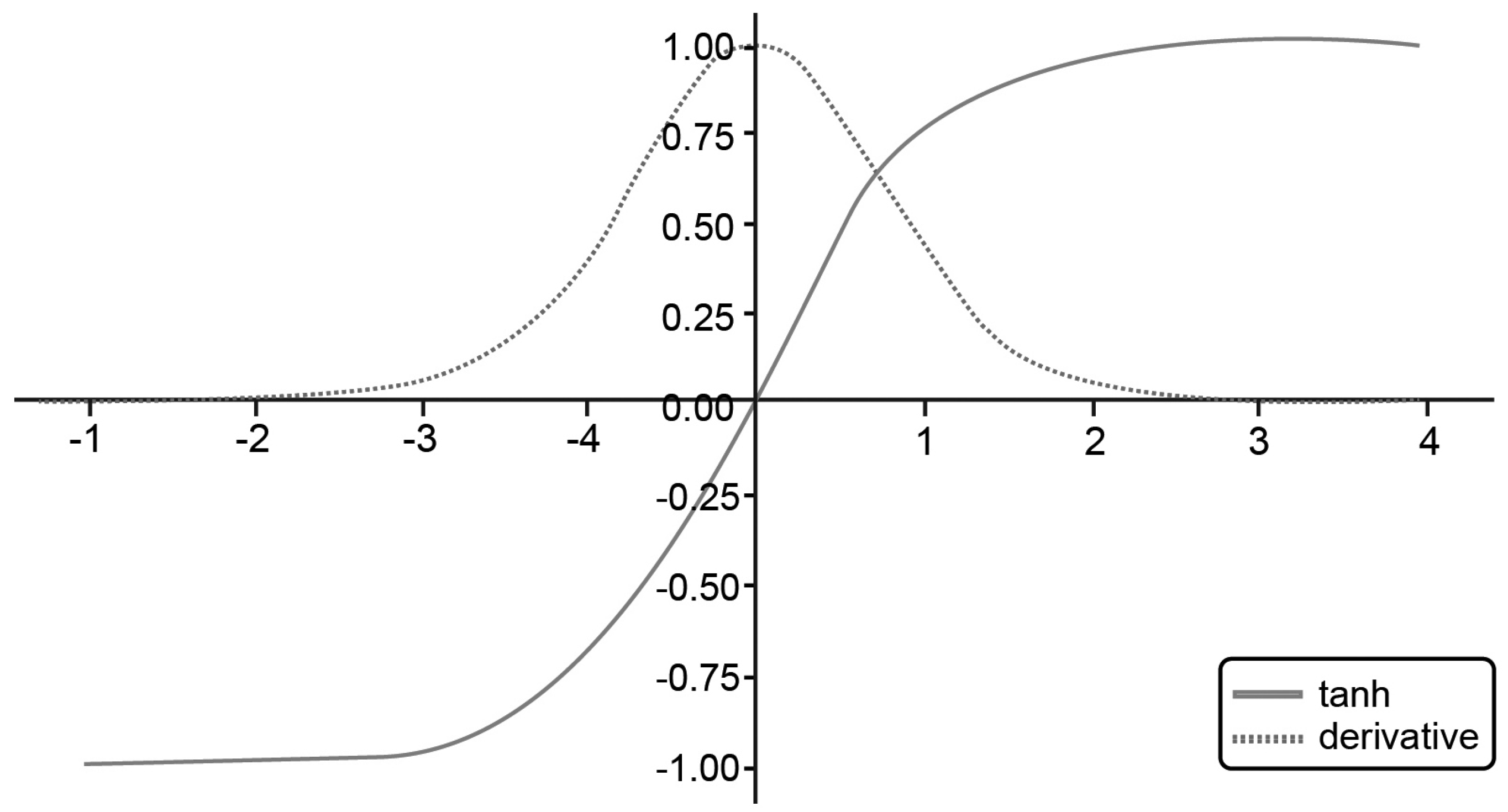
3.5.1. Tanh Activation Function

A widely used non-linear activation function that squashes the real-value to the range of [−1,1]. Figure 2 plots the graph of Tanh activation function and its derivative.

$$tanh\left(z\right)=\frac{e^z-e^{-z}}{e^z+e^{-z}}$$

(12)

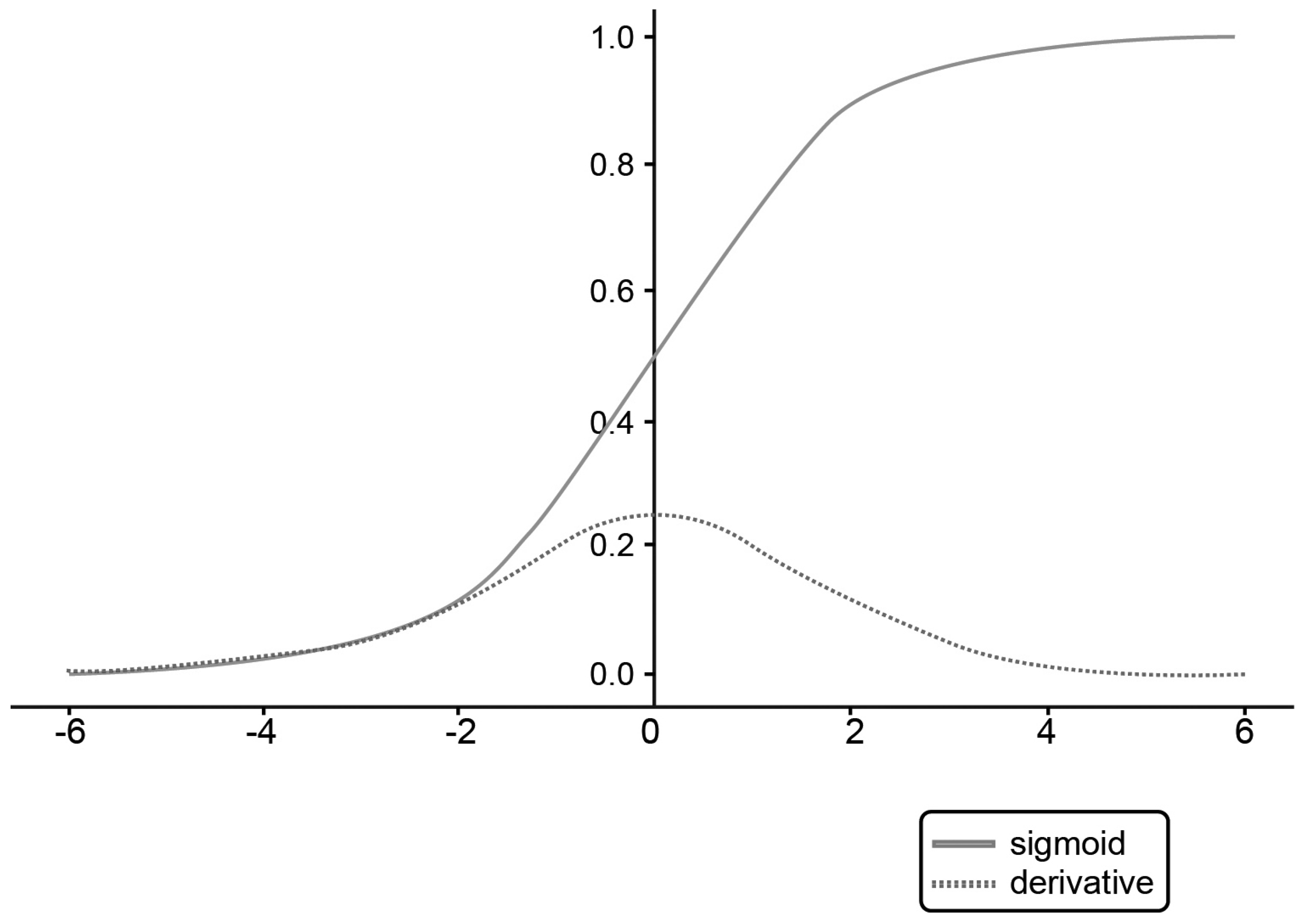
3.5.2. Sigmoid Activation Function

The monotonic activation function takes real values as input and outputs a value in the range [0,1] see Figure 3, gives a smooth gradient and is considered to be a good classifier.

$$S\left(z\right)=\frac{1}{1+e^{-z}}$$

(13)

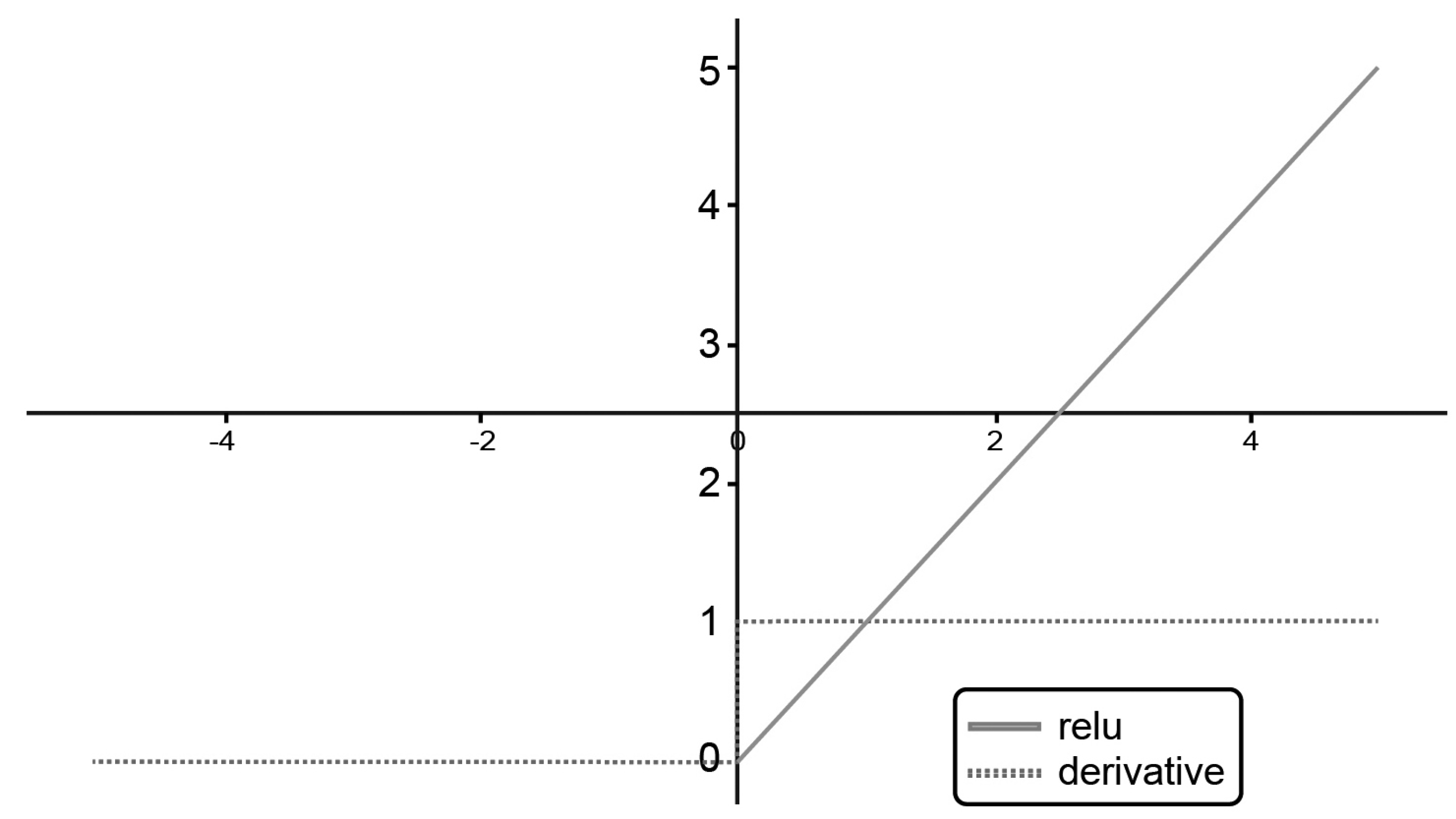
3.5.3. ReLU Activation Function

Rectified Linear Units abbreviated as ReLU is often chosen for its ability of handling vanishing gradient problems with the range of $[0,\infty ]$. Figure 4 shows the ReLU activation function and its derivative.

$$R\left(z\right)=\left\{\begin{array}{c}z\mathrm{if}z>0\hfill \\ 0\mathrm{if}z\le 0\hfill \end{array}\right.$$

(14)

3.6. Dataset

For the experiments, we have tried to include different datasets for the purpose of giving a generalization for the proposed combinations. Thus we did multi-organ segmentation as a part of testing this proposed approach. Apart from the liver data, we also used pancreas and cardiac data.

3.6.1. Liver—LiTS

The Liver Tumor Segmentation Challenge (LiTS) [43] dataset contains in-total of 201 contrast-enhanced 3D abdominal CT scans and ground truth segmentation for liver and lesions. The resolution of the images is considered to be 512 × 512 in each axial slice. For training, there exist 131 scans with ground-truth labels and 70 that can be used for testing. The slice spacing ranges from 0.45 mm to 5.0 mm and the in-plane resolution from 0.60 mm to 0.98 mm.

3.6.2. Medical Segmentation Decathlon

Medical Segmentation Decathlon(MSD) challenge datasets [44] consists of 10 different semantic segmentation tasks. Our experiments are based on only liver, pancreas and cardiac datasets. The liver dataset has 131 labeled volumes with two labels for segmenting liver and tumor from CT modality. The pancreas dataset has 282 labeled volumes for segmenting pancreas and tumor from CT modality. The cardiac dataset has 20 labeled volumes for segmenting the left atrium from MRI modality. The resolution of the liver and pancreas dataset is 512 × 512 and the resolution of the cardiac dataset is 320 × 320 pixels in each axial slice. All the datasets are scaled to an isotropic resolution of 1 × 1 × 1 mm and normalized to have zero mean and unit variance. The ground truth labels are binarized in the liver and pancreas dataset to only have liver and pancreas labels respectively.

3.7. Experiment 1

For the experiment, we used the implementation of VGG-16 implemented in Tensorflow for the purpose of segmenting the liver parenchyma in axial CT images. We have varied the activation functions in the hidden layers by applying the sigmoid $\frac{1}{(1+e^{-x})}$, hyperbolic tanh(x) and reLU functions. For the final layer we have applied Softmax function $s{\left(x\right)}_k=\frac{e^{x_k}}{{\sum }_{j=1}^n{e}^{x_j}}$. The initial learning rate $\left(lr\right)$ used here is $1\times {10}^{-4}$ and the weight decay is 0.0002. All the experiments are done using NVIDIA Tesla V100 (Nvidia, Sabta Clara, CA, USA) using public datasets SLIVER07 for the purpose of training and testing.

3.8. Experiment 2

In this experiment, the chainer implementation of the 3D U-Net is used to segment the liver parenchyma and pancreas parenchyma from CT volumes and left atrium from MRI volumes. The 3D patches of 64 × 64 × 64 were used as the input to the network. The different combinations of weight initialization methods along with different loss functions and optimizers have been experimented with. We used Glorot, He and LeCun initialization methods, in combination with loss functions including Softmax cross-entropy and Dice loss, and optimizers including Adam and RMSProp. In total, 12 different combinations have been experimented with for each dataset. We used the initial learning rate of 0.0001 and ReLU activation for all the combinations of this experiment. The Medical Segmentation Decathlon (MSD) challenge datasets were used for the purpose of training, validation and testing in this experiment. The models for all the combinations were trained on the NVIDIA DGX2 server with Tesla Volta GPUs.

As both the experiments were done simultaneously, we employed two different servers for handling the computations. Also, in our experiments, we used 70% data for training, 20% for validation and 10% for testing.

3.9. Segmentation Evaluation Methods

In order to compare different configurations, we have selected eight evaluation metrics. These include spatial overlap-based assessment methods like DICE, spatial distance-based metrics like Hausdorff Distance (HD), Average Hausdorff Distance (AVD) and Mahalanobis distance (MD), information theoretic-based measures like Mutual Information (MI) and Variation of Information (VOI), probabilistic measure like Area under ROC curve (AUC) and finally volume-based called Volumetric Similarity (VS). The selection of these metrics is based on the target of the segmentation methods being applied for this study based on the recommendations given in [35].

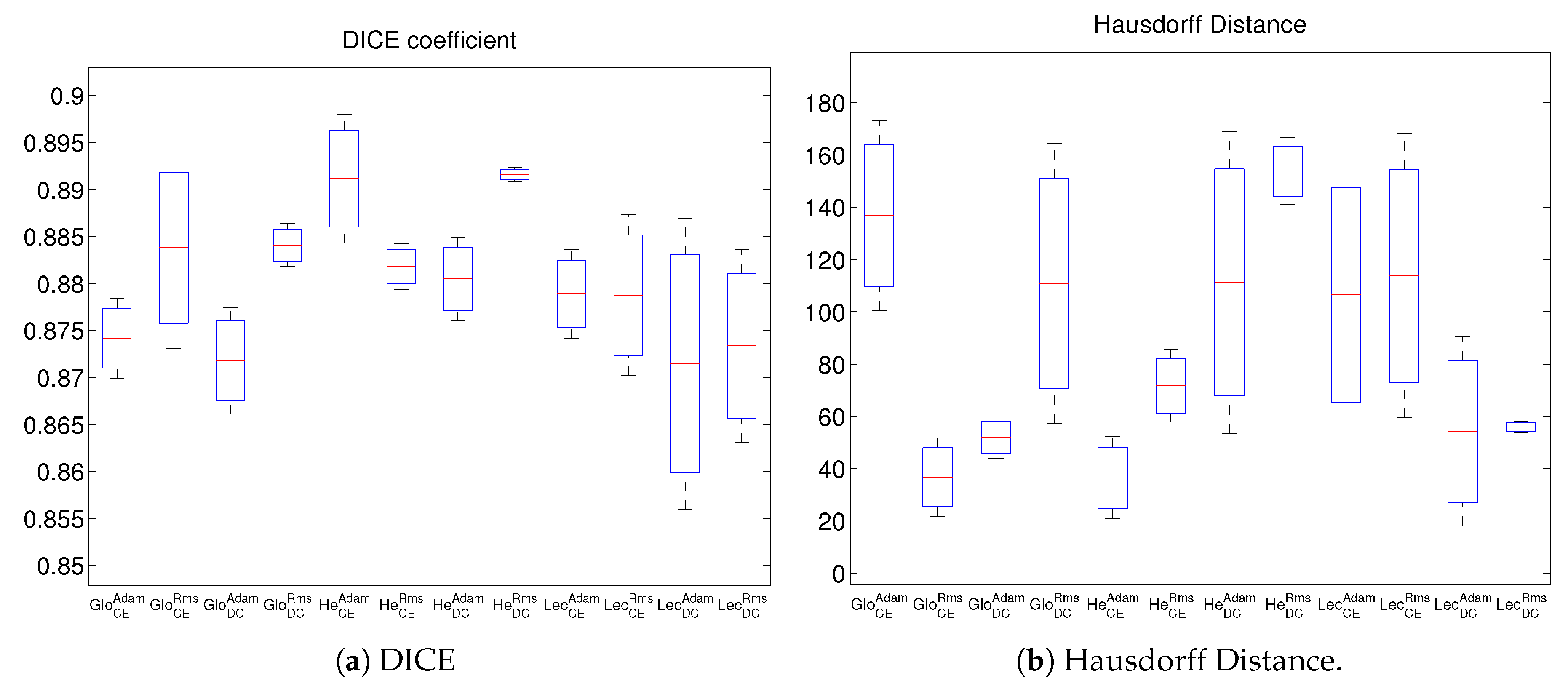
3.9.1. Dice Coefficient (DICE)

The Dice coefficient (DICE) is the most commonly used metric for validation of medical image segmentation [35]. It is used to find the overlap between the ground-truth segmentation $S_g$ and the test segmentation $S_t$ using

$$\mathrm{DICE}=\frac{2|S_g\cap S_t|}{|S_g|+|S_t|}$$

(15)

where $|S_g|$ and the $|S_t|$ are the cardinalities of the two sets.

3.9.2. Hausdorff Distance (HD)

The Hausdorff Distance (HD) [45] is a spatial-distance based metric used to evaluate dissimilarity between two segmentation contours. Like other distance-based measures, the spatial distance is measured using spatial positions of the voxels. For two finite point sets, HD is defined in terms of directed Hausdorff distance $h(A,B)$ as

$$\mathrm{HD}(A,B)=max\left(h\right(A,B),h(A,B\left)\right)$$

(16)

where

$$h(A,B)=\underset{a\in A}{max}\underset{b\in B}{min}\left|\right|a-b\left|\right|$$

(17)

with $\left|\right|.\left|\right|$ is some norm like the Euclidean distance. A smaller value of HD implies better segmentation results.

3.9.3. Average Hausdorff Distance (AVD)

One of the drawbacks of HD is that it is sensitive to outliers. Average Hausdorff Distance (AVD) [45], as the name suggests, is the average of HD for all points. AVD is generally more stable and is defined as

$$\mathrm{AVD}(A,B)=max\left(d\right(A,B),d(A,B\left)\right)$$

(18)

where $d(A,B)$ is the directed average Hausdorff distance defined as

$$d(A,B)=\frac{1}{N}\sum _{a\in A}\underset{b\in B}{min}\left|\right|a-b\left|\right|$$

(19)

3.9.4. Mahalanobis Distance (MHD)

Mahalanobis Distance (MHD) [46] uses the means of two comparing point clouds (segmented images) ${\mu }_A$ and $m{u}_B$ and their common covariance matrix S to give the following distance measure

$$\mathrm{MHD}(A,B)=\sqrt{{({\mu }_A-{\mu }_B)}^T{S}^{-1}({\mu }_A-{\mu }_B)}$$

(20)

where common covariance matrix S is given as

$$S=\frac{{\alpha }_1{S}_1+{\alpha }_2{S}_2}{{\alpha }_1+{\alpha }_2}$$

(21)

In the above equation, $S_1$ and $S_2$ are the co-variance matrices of sets of voxels with ${\alpha }_1$ and ${\alpha }_2$ number of voxels respectively.

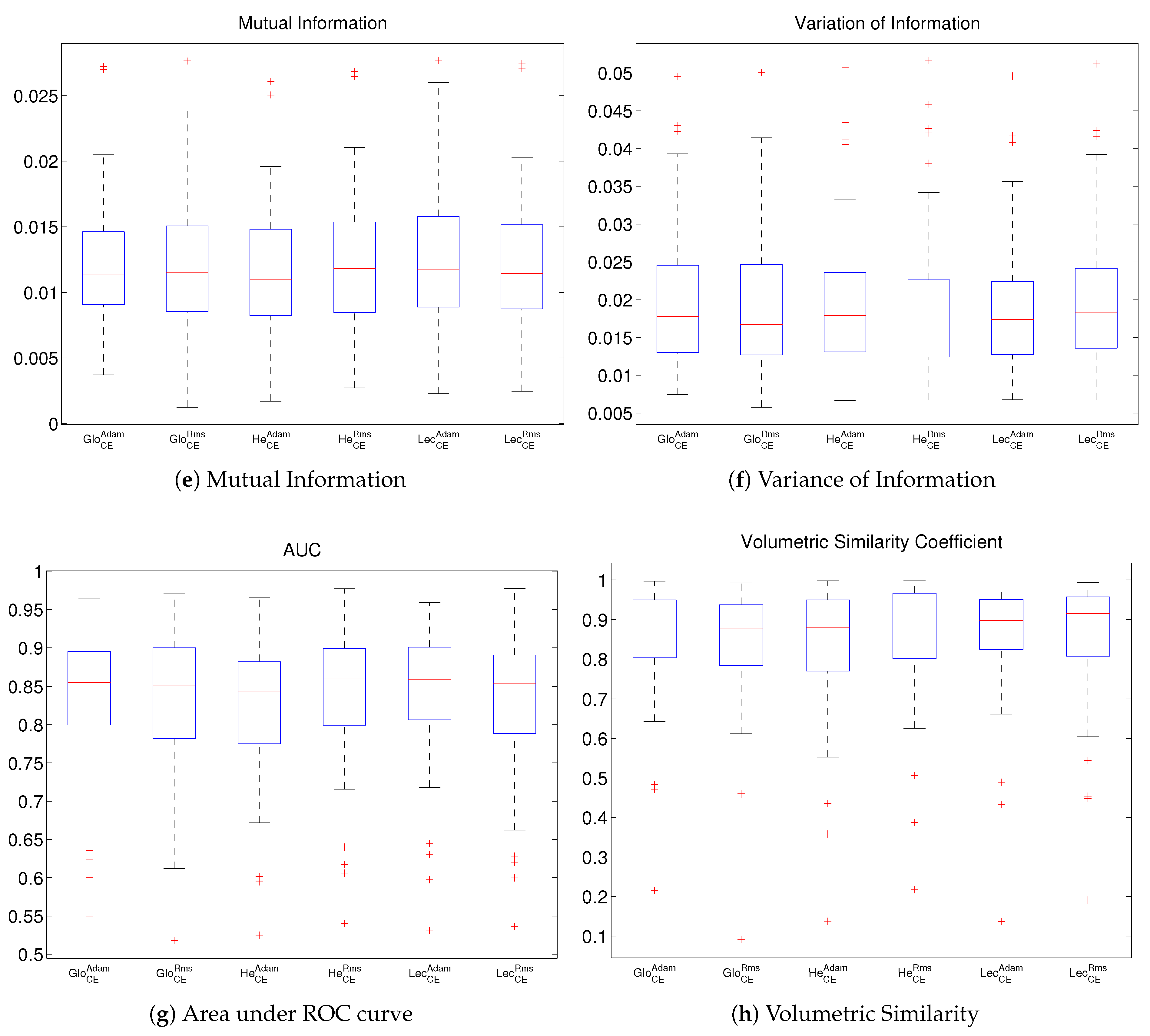
3.9.5. Mutual Information (MI)

In information theory, Mutual information (MI) between two random variables provides a measure of the amount of information that can be obtained about one variable by looking at the other. It can also be used to find similarity between two segmentation [47]. It is linked to the marginal entropies $H\left(S_g\right)$ and $H\left(S_t\right)$ and the joint entropy $H(S_g,S_t)$ of the two variables, i.e., segmented images $S_g$ and $S_t$ and is defined as

$$\mathrm{MI}(S_g,S_t)=H\left(S_g\right)+H\left(S_t\right)-H(S_g,S_t)$$

(22)

3.9.6. Variation of Information (VOI)

This is another information-theory based measure. The Variation of Information (VOI) [48] is based on marginal entropies and MI and provides a measure of gain or loss in information when changing from one variable to another. It is defined by the following equation

$$\mathrm{VOI}(S_g,S_t)=H\left(S_g\right)+H\left(S_t\right)-2\mathrm{MI}(S_g,S_t)$$

(23)

3.9.7. Area under ROC Curve (AUC)

Receiver Operating Curve (ROC) is a plot of True Positive Rate (TPR) against False Positive Rate (FPR). In the case of segmentation, TPR refers to the ratio of positive (foreground/segmented) voxels identified correctly out of the total number of positive voxels in the ground-truth. Similarly, FPR refers to the ratio of voxels identified incorrectly as positives out of the total number of negative (background) voxels in the ground-truth. The area under ROC curve (AUC) is a measure of separability for a classifier telling how well it is in distinguishing between classes (positive and negative voxels). Based on the definition by [49], AUC is defined as

$$\mathrm{AUC}=1-\frac{1}{2}(\frac{FP}{FP+TN}+\frac{FN}{FN+TP})$$

(24)

where $FP$, $TN$, $FN$ and $TP$ refer to as False Positive, True Negative, False Negative and True Positive respectively.

3.9.8. Volumetric Similarity (VS)

Volumetric Similarity (VS) is used to compare the volume of segmented regions in the two images. The volumes used for comparison are the absolute ones and not only of the overlapped regions. It is evaluated by subtracting from 1 the volumetric distance which is defined as the absolute difference between two volumes divided by the sum of the two [50]

$$\mathrm{VS}(S_g^R,S_t^R)=1-\frac{\left|\right|S_t^R|-|S_g^R\left|\right|}{|S_t^R|+|S_g^R|}$$

(25)

4. Experimental Results and Discussion

We performed segmentation of different organs data using two different networks 3D-UNet and VGG-16. The former has been used for the segmentation of cardiac, liver and pancreas whereas the latter for the segmentation of the liver alone. The 3D-UNet model used for the segmentation of different organs has been tested with a combinatorial approach of weight initialization methods together with loss functions and optimizers. For the liver segmentation model, we used the approach of combining weight initialization with activation functions. From both the experiments we tried to gather information using different evaluation metrics. This has been done, as it is hard to set an optimal parameter value that says the segmentation obtained from the particular combination works better. So we decided to choose multiple sets of quality assessment metrics. Figure 5 and Figure 6 shows the predictions from both best combinations that gives high Dice score and those that gives lower values of Dice score displayed using ITK-SNAP Viewer [51]. These visualizations of the results conveys the significant difference of each choices made. It is possible to view the qualitative results from these experiments on ITK-SNAP in four different views axial, coronal, sagittal and the 3D view of predictions (see Figure 7).

Comparison and Discussion of Results

In order to assess and compare the results of segmentations resulting from different combinations of hyper-parameters, we have used the eight evaluation metrics described in Section 3.9. The metrics have been evaluated using the VISCERAL evaluation software package [35].

Table 1. Mean and standard deviation values for Segmentation metrics on Liver Database (higher values represented in bold and lower values in italics with underline).

Configuration	DICE	HD	AVD	MHD	MI	VOI	AUC	VS
GloCEAdam	0.897 ± 0.100	291.24 ± 93.73	2.553 ± 3.02	0.163 ± 0.153	0.138 ± 0.076	0.071 ± 0.057	0.938 ± 0.069	0.952 ± 0.107
GloCERms	0.870 ± 0.191	298.39 ± 96.38	3.62 ± 4.15	0.200 ± 0.194	0.133 ± 0.078	0.076 ± 0.066	0.929 ± 0.101	0.927 ± 0.200
GloDCRms	0.866 ± 0.147	316.81 ± 74.69	4.33 ± 4.75	0.213 ± 0.156	0.131 ± 0.076	0.082 ± 0.062	0.925 ± 0.087	0.936 ± 0.153
HeCEAdam	0.871 ± 0.146	293.74 ± 95.25	2.88 ± 2.96	0.183 ± 0.160	0.131 ± 0.074	0.081 ± 0.065	0.923 ± 0.087	0.937 ± 0.155
HeCERms	0.863 ± 0.205	295.67 ± 96.23	4.24 ± 4.68	0.232 ± 0.261	0.132 ± 0.079	0.078 ± 0.063	0.929 ± 0.105	0.923 ± 0.216
HeDCAdam	0.858 ± 0.177	294.17 ± 77.70	3.60 ± 4.00	0.208 ± 0.236	0.129 ± 0.077	0.082 ± 0.065	0.916 ± 0.097	0.925 ± 0.185
HeDCRms	0.860 ± 0.185	297.14 ± 101.46	3.82 ± 4.03	0.203 ± 0.173	0.129 ± 0.076	0.082 ± 0.066	0.921 ± 0.099	0.924 ± 0.196
LecCEAdam	0.883 ± 0.148	287.11 ± 89.97	2.40 ± 2.73	0.160 ± 0.150	0.134 ± 0.078	0.073 ± 0.062	0.929 ± 0.087	0.935 ± 0.156
LecCERms	0.873 ± 0.168	295.23 ± 99.38	3.47 ± 4.10	0.210 ± 0.220	0.133 ± 0.078	0.076 ± 0.062	0.928 ± 0.094	0.934 ± 0.177
LecDCAdam	0.860 ± 0.191	302.52 ± 95.88	3.80 ± 4.01	0.214 ± 0.217	0.130 ± 0.078	0.081 ± 0.064	0.921 ± 0.100	0.928 ± 0.202
LecDCRms	0.867 ± 0.199	311.64 ± 76.32	3.54 ± 4.23	0.204 ± 0.226	0.133 ± 0.080	0.076 ± 0.062	0.926 ± 0.102	0.927 ± 0.209

,

Table 2. Mean and standard deviation values for Segmentation metrics on Heart Database (higher values represented in bold and lower values in italics with underline).

Configuration	DICE	HD	AVD	MHD	MI	VOI	AUC	VS
GloCEAdam	0.874 ± 0.006	136.84 ± 51.41	0.374 ± 0.078	0.132 ± 0.005	0.025 ± 0.004	0.014 ± 0.003	0.916 ± 0.002	0.948 ± 0.014
GloCERms	0.884 ± 0.015	36.76 ± 21.20	0.310 ± 0.021	0.084 ± 0.007	0.026 ± 0.003	0.013 ± 0.004	0.921 ± 0.007	0.951 ± 0.001
GloDCAdam	0.872 ± 0.008	52.04 ± 11.46	0.658 ± 0.367	0.174 ± 0.096	0.025 ± 0.004	0.015 ± 0.002	0.919 ± 0.005	0.961 ± 0.004
GloDCRms	0.884 ± 0.003	110.88 ± 75.91	0.494 ± 0.168	0.146 ± 0.055	0.026 ± 0.004	0.014 ± 0.003	0.792 ± 0.005	0.964 ± 0.019
HeCEAdam	0.891 ± 0.010	36.44 ± 22.20	0.311 ± 0.013	0.101 ± 0.019	0.026 ± 0.004	0.013 ± 0.003	0.927 ± 0.001	0.957 ± 0.008
HeCERms	0.882 ± 0.003	71.70 ± 19.61	0.360 ± 0.015	0.143 ± 0.015	0.026 ± 0.004	0.014 ± 0.003	0.921 ± 0.010	0.954 ± 0.028
HeDCAdam	0.881 ± 0.006	111.29 ± 81.84	0.359 ± 0.101	0.115 ± 0.031	0.026 ± 0.004	0.014 ± 0.003	0.922 ± 0.003	0.957 ± 0.015
HeDCRms	0.892 ± 0.001	153.89 ± 18.03	0.310 ± 0.012	0.117 ± 0.050	0.026 ± 0.004	0.013 ± 0.002	0.929 ± 0.006	0.961 ± 0.013
LecCEAdam	0.879 ± 0.007	106.52 ± 77.41	0.375 ± 0.107	0.101 ± 0.003	0.026 ± 0.004	0.014 ± 0.003	0.919 ± 0.002	0.951 ± 0.015
LecCERms	0.879 ± 0.012	113.72 ± 76.83	0.568 ± 0.346	0.155 ± 0.074	0.026 ± 0.005	0.014 ± 0.002	0.918 ± 0.017	0.949 ± 0.028
LecDCAdam	0.871 ± 0.022	54.26 ± 51.20	0.414 ± 0.149	0.142 ± 0.095	0.025 ± 0.005	0.014 ± 0.001	0.914 ± 0.022	0.946 ± 0.030
LecDCRms	0.873 ± 0.014	55.87 ± 3.03	0.341 ± 0.051	0.145 ± 0.066	0.025 ± 0.005	0.014 ± 0.002	0.911 ± 0.019	0.936 ± 0.033

and

Table 3. Mean and standard deviation values for Segmentation metrics on Pancreas Database (higher values represented in bold and lower values in italics with underline).

Configuration	DICE	HD	AVD	MHD	MI	VOI	AUC	VS
GloCEAdam	0.679 ± 0.148	117.03 ± 50.96	4.02 ± 6.83	0.382 ± 0.262	0.012 ± 0.005	0.020 ± 0.010	0.834 ± 0.098	0.848 ± 0.159
GloCERms	0.681 ± 0.156	119.79 ± 56.51	3.49 ± 7.03	0.370 ± 0.251	0.012 ± 0.005	0.020 ± 0.010	0.827 ± 0.099	0.834 ± 0.173
HeCEAdam	0.659 ± 0.165	117.58 ± 51.82	3.89 ± 5.94	0.372 ± 0.266	0.012 ± 0.005	0.020 ± 0.010	0.814 ± 0.104	0.826 ± 0.187
HeCERms	0.686 ± 0.156	111.14 ± 52.88	3.623 ± 7.14	0.339 ± 0.257	0.013 ± 0.005	0.020 ± 0.011	0.836 ± 0.099	0.849 ± 0.168
LecCEAdam	0.691 ± 0.148	121.52 ± 57.92	2.97 ± 4.25	0.325 ± 0.264	0.013 ± 0.006	0.019 ± 0.009	0.837 ± 0.097	0.848 ± 0.168
LecCERms	0.672 ± 0.156	117.91 ± 50.82	3.74 ± 5.23	0.357 ± 0.274	0.012 ± 0.005	0.020 ± 0.010	0.825 ± 0.102	0.845 ± 0.171

show the mean values of metrics for each configuration applied to liver, heart and pancreas databases respectively. These configurations vary in initialization, loss function and optimizer used. Each configuration in these tables is represented using the notation like $Ini{t}_{loss}^{optim}$ where $Init=\{Glo,He,Lec\}$, $loss=\{DC,CE\}$ and $optim=\{Adam,Rms\}$. Here $Glo$ and $Lec$ are short names used for Glorot and LeCun initializations and $DC$ and $CE$ are used for Dice loss, and Cross-entropy loss respectively.

Table 4. Mean and standard deviation values for Segmentation metrics on LiTS Database (higher values represented in bold and lower values in italics with underline).

Configuration	DICE	HD	AVD	MHD	MI	VOI	AUC	VS
Glotanh	0.921 ± 0.034	474.95 ± 131.44	1.32 ± 2.08	0.302 ± 0.179	0.124 ± 0.048	0.056 ± 0.050	0.969 ± 0.026	0.962 ± 0.031
RandNormrelu	0.853 ± 0.063	499.38 ± 92.03	2.30 ± 1.92	0.507 ± 0.190	0.113 ± 0.030	0.093 ± 0.078	0.951 ± 0.053	0.906 ± 0.067
Hesigm	0.857 ± 0.063	511.43 ± 92.94	2.40 ± 2.43	0.515 ± 0.201	0.110 ± 0.034	0.087 ± 0.072	0.952 ± 0.047	0.913 ± 0.061

on the other hand gives a comparison combining weight initialization choices with combination of activation functions. The configurations we used in the table are represented using notations $Ini{t}_{activation}$, whereas the initialization constitutes $Init=\{Glo,RandNorm,He\}$ and activation functions consist of $activation=\{tanh,relu,sigm\}$. We have represented all the parameters used in this study in

Table A1. Parameters experimented under each category, and their abbreviations.

Weight Initialization	Activation Function	Loss Function	Optimizer
Xavier or Glorot (Glo)	Tanh (tanh)	Cross Entropy (CE)	Adam (Adam)
He Initialization (He)	ReLU (relu)	Dice loss (DC)	RMSprop (Rms)
LeCun (Le)	Sigmoid (sigm)
Random Normal (RandNorm)

.

It is important to note that in each of Table 1, Table 2 and Table 3 only those configurations have been included for which there was a segmentation result obtained. Hence configuration $Gl{o}_{DC}^{Adam}$ for the liver database and all Dice-loss-based configurations for the pancreas database have not been considered. The values in bold in these tables highlight the best two values for each metric whereas those in italics with an underline depict the worst value. Overall we see small (but mostly statistically significant) differences in the values of most of the metrics. However, from Table 1 we can observe that both $Gl{o}_{CE}^{Adam}$ and $Le{c}_{CE}^{Adam}$ have been evaluated as the best by all the metrics. On the contrary, both $Gl{o}_{DC}^{Rms}$ and $H{e}_{DC}^{Adam}$ give the worst results for at least four of the total eight metrics.

These conclusions can further be verified using the box plots for all metrics as illustrated in Figure 8. From the box plot of DICE, it can be observed that the results for both $Gl{o}_{CE}^{Adam}$ and $Le{c}_{CE}^{Adam}$ are more consistent having a small inter-quartile range and are also uniformly spread around the median value. The outliers for these two configurations are also fewer and less far away from the minimum value. The same trend of a smaller inter-quartile range can also be seen for other metrics like AVD, MHD and AUC. Contrary to that, looking at the configurations which have the worst mean values, they tend to have a larger spread for most metrics. The results further indicate that the use of the Cross-entropy loss function has a better performance as compared to DICE for liver segmentation. This can be easily verified from the table and the box plots if we compare each pair of configurations having the same initialization and optimizer function but differing in the loss function.

Even for the segmentation results for the pancreas, the use of DICE as a loss function failed to give any results for any configuration. From amongst the remaining configurations, we observe that $Le{c}_{CE}^{Adam}$ again performs amongst the best as can be seen in Table 3. However, in this case, it is accompanied as the second-best by configuration using He initialization with RMSProp optimization, i.e., $H{e}_{CE}^{Rms}$. The box plots in Figure 9 also illustrate that for the majority of metrics these two configurations have a smaller spread as compared to the others.

For the heart database, we can see from Table 2 that the configuration $H{e}_{CE}^{Adam}$ gives the best results. Two other configurations of $Gl{o}_{CE}^{Rms}$ and $H{e}_{DC}^{Rms}$ also fare better than the other configurations in terms of at least three metrics excluding the non-discriminant metrics of MI and VOI. From Figure 10, it is visible that $H{e}_{CE}^{Adam}$ gives good consistency and better values for DICE, HD, AVD, AUC and VS. $Gl{o}_{CE}^{Rms}$ has a good performance with HD, AVD, MHD and VS whereas $H{e}_{DC}^{Rms}$ gives better values and consistency for DICE, AVD, AUC and VS. Hence, for the heart database we see a discrepancy that a configuration with DICE as loss function is also amongst one of the better configurations. However, it is important to note here also that the testing dataset for the heart database was also very small as compared to the other two and it could be interesting to see the results with a bigger dataset.

Table 4 shows a comparison of the two configurations on LiTS dataset which differ in initialization and activation functions. Amongst the two configurations, we can clearly observe that $Gl{o}_{tanh}$ outperforms the $RandNor{m}_{relu}$ and $H{e}_{sigm}$ configuration.

In order to verify the statistical significance of the differences between the multiple configurations, we have further performed a paired t-test of the best configuration with each of the other configurations for each dataset. This test is performed for each of the eight quality metrics used. The null hypothesis for the paired t-test is rejected when $p\le 0.05$. However, due to the limited data in the case of Heart database, we haven’t performed statistical analysis on its results.

Table 5. Statistical Significant differences ($p\le 0.05$) denoted by checkmark for each configuration in comparison to $Gl{o}_{CE}^{Adam}$ for Liver Dataset.

Configuration	DICE	HD	AVD	MHD	MI	VOI	AUC	VS
GloCERms			✓	✓		✓
GloDCRms	✓	✓	✓	✓	✓	✓	✓
HeCEAdam	✓		✓	✓	✓	✓	✓
HeCERms			✓	✓		✓
HeDCAdam	✓		✓	✓	✓	✓	✓
HeDCRms	✓		✓	✓	✓	✓	✓
LecCEAdam					✓		✓
LecCERms			✓	✓	✓	✓
LecDCAdam	✓		✓	✓	✓	✓	✓
LecDCRms		✓	✓	✓		✓

shows the comparisons with $Gl{o}_{CE}^{Adam}$ configuration for the Liver Dataset. The checkmarks in the table denote that the p-value is less than or equal to 0.05 implying statistical significance in differences. From the table, we can see that except for VS and HD all the metrics show that by selecting different loss functions, initializations and optimizers, the improvements in the output are significant. Moreover, as expected, for the $L{e}_{CE}^{Adam}$, which was the second best configuration and hence closer to the $Gl{o}_{CE}^{Adam}$ in terms of results, we see none of the metric values to be significantly different except MI. Additionally, we also see from Table 5 that for all initializations with a combination of $CE$ loss and $Rms$ optimizer, both DICE and AUC do not change significantly but the AVD, MHD, MI and VOI provide an insight into the significant changes in outcomes between these configurations.

Similarly,

Table 6. Statistical Significant differences ($p\le 0.05$) denoted by checkmark for each configuration in comparison to $Le{c}_{CE}^{Adam}$ for Pancreas Dataset.

Configuration	DICE	HD	AVD	MHD	MI	VOI	AUC	VS
GloCEAdam	✓		✓	✓	✓
GloCERms	✓			✓		✓	✓
HeCEAdam	✓		✓	✓	✓	✓	✓	✓
HeCERms		✓
LecCERms	✓		✓		✓	✓

shows the statistical analysis results for the Pancreas dataset with checkmarks highlighting statistical significance in comparison to the best $Le{c}_{CE}^{Adam}$ configuration. Here again we can observe that both HD and VS metrics mostly do not show significant differences except for the case where the best and the worst configurations are compared to each other. The p-value of less than 0.5 for all the rest of the metrics in most cases signify that the choice of parameters does have a noticeable impact on improving the segmentation results for Pancreas database. Moreover, with similar results as for the case of the second best configuration of $H{e}_{CE}^{Rms}$, the null hypothesis is not rejected for the majority of the metrics used.

Finally, we have performed paired t-tests on the values in Table 4 for the comparison of configurations varying in initialization and activation functions. The comparison was performed between each configuration and the best one, i.e., $Gl{o}_{tanh}$.

Table 7. p-Values for t-test with $Gl{o}_{tanh}$ performed for Segmentation metrics on LiTS Database.

Configuration	DICE	HD	AVD	MHD	MI	VOI	AUC	VS
RandNormrelu	4.43 $\times {10}^{-8}$	6.74 $\times {10}^{-4}$	4.14 $\times {10}^{-3}$	1.05 $\times {10}^{-9}$	4.36 $\times {10}^{-3}$	6.82 $\times {10}^{-6}$	1.36 $\times {10}^{-2}$	2.83 $\times {10}^{-6}$
Hesigm	9.75 $\times {10}^{-8}$	5.97 $\times {10}^{-4}$	1.36 $\times {10}^{-3}$	1.12 $\times {10}^{-9}$	1.42 $\times {10}^{-3}$	2.61 $\times {10}^{-6}$	4.71 $\times {10}^{-3}$	1.45 $\times {10}^{-6}$

shows the p-values for all the metrics. From the table, we can clearly see that for all the metrics the p-values are much lower than the significance value of 0.05. This suggests that the null hypothesis is rejected and there are significant differences between the best configuration and the rest in terms of segmentation results.

As we can see, the configurations used for both the experiments are different from each other and we employed 3D-UNet for multi-dataset segmentation as well as VGG-16 based segmentation model for a single dataset study. We have seen in the literature [11,12,13,14], the most promising successor of FCN is 3D-UNet. Used widely for multi-class segmentation [52,53] and often referred to as a universal segmentation model, we decided to follow the same idea of employing 3D-UNet for multi-dataset segmentation. We used different combinations of the parameters including weight initialization, loss functions and optimizers keeping ReLU as the activation function considering two main reasons.According to the literature, ReLU performed well with the U-Net architecture [54,55] and is considered to be six times faster than sigmoid/tanh activation functions. Here, as we were handling multi-dataset we need to reduce the computational cost, hence followed the principle of keeping ReLU as the activation function for all the experiments carried out in 3D-UNet. For the single dataset study on VGG-16 based segmentation model, we followed the combinations or activation functions combined with weight initialization keeping the loss function constant (CE). Although, VGG-16 is considered to be best for classification tasks, here we tried to come up with a solution for liver segmentation together with a study of parameter choices. “Training algorithms for deep learning models are usually iterative in nature and thus require the user to specify some initial point from which to begin the iterations. Moreover, training deep models is a sufficiently difficult task that most algorithms are strongly affected by the choice of initialization” [56], as mentioned in this statement, the motivation was to propose a better initialization scheme that works with the activation function. From the observations from the quality matrices, we could agree that the tanh activation function can be a good alternative to sigmoid and works well with Glorot/Xavier weight initialization [55].

5. Conclusions

In this research work, chainer implementation of 3D-UNet and VGG-16 networks were applied for segmentation tasks of the medical image dataset. The main observations from the experiments conducted show that perhaps there are interactions between the architectural parameters that enhance the output scores. The research work has been concentrated more on initialization schemes rather than the famous hyper-parameter searching techniques. We made two different approaches, a multi-dataset segmentation study and single-dataset segmentation evaluation. From both the experiments, we propose few of the combinations that may work better for segmentation results although it is hard to make a concise conclusion from the values in quality matrices. In best of our knowledge, there is no best algorithm proposed for the purpose of generalised medical image segmentation, but studies show that there can be best choices we can make while designing the architecture [22,23,24]. From our experimental results, we have observed that two of the combinations with Xavier weight initialization (also known as Glorot), Adam optimiser, Cross Entropy loss ($Gl{o}_{CE}^{Adam}$) and LeCun weight initialization, cross entropy loss and Adam optimiser $Le{c}_{CE}^{Adam}$ worked best for most of the metrics in 3D-UNet setting, while Xavier together with cross entropy loss and Tanh activation function ($Gl{o}_{CE}^{tanh}$) worked best for VGG-16 network. The quantitative and qualitative analysis performed during the development of this work (see Table 1, Table 2, Table 3, Table 4, Table 5, Table 6 and Table 7 and Figure 5 and Figure 6) shows the significant importance of the proposed combinations for the future development and designing of network architectures. We believe that this research can provide new perspective for the related researches in the medical domain, and also help fellow researchers to choose appropriate combinations for their network structure and to be aware of the possible challenges and the solutions. As an extension to this work, we would like to experiment with the combinations with better results on a multi-domain network that works for segmentation analysis in data from two different domains, for example, CT/MR images.

References

1. Galloway, R.L.; Herrell, S.D.; Miga, M.I. Image-guided abdominal surgery and therapy delivery. J. Healthc. Eng. 2012, 3, 203–228. [Google Scholar] [CrossRef] [Green Version]
2. Warfield, S.K.; Jolesz, F.A.; Kikinis, R. Real-time image segmentation for image-guided surgery. In Proceedings of the 1998 ACM/IEEE Conference on Supercomputing (SC’98), Orlando, FL, USA, 7–13 November 1998; p. 42. [Google Scholar]
3. Grimson, W.E.L.; Leventon, M.E.; Faugeras, O.D.; Wells, W.; Mirmehdi, M.; Thomas, B. Computer Vision Methods for Image Guided Surgery. In Proceedings of the BMVC, Bristol, UK, 11–14 September 2000; pp. 1–12. [Google Scholar]
4. Zhou, Z.; Xue-Chang, Z.; Si-Ming, Z.; Hua-Fei, X.; Yue-Ding, S. Semi-automatic Liver Segmentation in CT Images through Intensity Separation and Region Growing. Procedia Comput. Sci. 2018, 131, 220–225. [Google Scholar] [CrossRef]
5. Hesamian, M.H.; Jia, W.; He, X.; Kennedy, P. Deep Learning Techniques for Medical Image Segmentation: Achievements and Challenges. J. Digit. Imaging 2019, 32. [Google Scholar] [CrossRef] [PubMed] [Green Version]
6. Roth, H.R.; Shen, C.; Oda, H.; Oda, M.; Hayashi, Y.; Misawa, K.; Mori, K. Deep learning and its application to medical image segmentation. Med. Imaging Technol. 2018, 36, 63–71. [Google Scholar]
7. Talbi, E.G. Optimization of Deep Neural Networks: A Survey and Unified Taxonomy. 2020. Available online: https://hal.inria.fr/hal-02570804v2 (accessed on 8 December 2020).
8. Christ, P.F.; Elshaer, M.E.A.; Ettlinger, F.; Tatavarty, S.; Bickel, M.; Bilic, P.; Rempfler, M.; Armbruster, M.; Hofmann, F.; D’Anastasi, M.; et al. Automatic liver and lesion segmentation in CT using cascaded fully convolutional neural networks and 3D conditional random fields. In Proceedings of the International Conference on Medical Image Computing and Computer-Assisted Intervention, Athens, Greece, 17–21 October 2016; Springer: Berlin/Heidelberg, Germany, 2016; pp. 415–423. [Google Scholar]
9. Shen, D.; Wu, G.; Suk, H.I. Deep Learning in Medical Image Analysis. Annu. Rev. Biomed. Eng. 2017, 19, 221–248. [Google Scholar] [CrossRef] [PubMed] [Green Version]
10. Litjens, G.; Kooi, T.; Bejnordi, B.E.; Setio, A.A.A.; Ciompi, F.; Ghafoorian, M.; Van Der Laak, J.A.; Van Ginneken, B.; Sánchez, C.I. A survey on deep learning in medical image analysis. Med. Image Anal. 2017, 42, 60–88. [Google Scholar] [CrossRef] [Green Version]
11. Çiçek, Ö.; Abdulkadir, A.; Lienkamp, S.S.; Brox, T.; Ronneberger, O. 3D U-Net: Learning Dense Volumetric Segmentation from Sparse Annotation. In Proceedings of the International Conference on Medical Image Computing and Computer-Assisted Intervention, Athens, Greece, 17–21 October 2016; Springer: Cham, Switzerland, 2016. [Google Scholar]
12. Shelhamer, E.; Long, J.; Darrell, T. Fully convolutional networks for semantic segmentation. IEEE Trans. Pattern Anal. Mach. Intell. 2017, 39, 640–651. [Google Scholar] [CrossRef]
13. Zhu, W.; Huang, Y.; Zeng, L.; Chen, X.; Liu, Y.; Qian, Z.; Du, N.; Fan, W.; Xie, X. AnatomyNet: Deep learning for fast and fully automated whole-volume segmentation of head and neck anatomy. Med. Phys. 2019, 46, 576–589. [Google Scholar] [CrossRef] [Green Version]
14. Milletari, F.; Navab, N.; Ahmadi, S.A. V-net: Fully convolutional neural networks for volumetric medical image segmentation. In Proceedings of the 2016 IEEE Fourth International Conference on 3D Vision (3DV), Stanford, CA, USA, 25–28 October 2016; pp. 565–571. [Google Scholar]
15. Simonyan, K.; Zisserman, A. Very deep convolutional networks for large-scale image recognition. arXiv 2014, arXiv:1409.1556. [Google Scholar]
16. Aguirre, D. A Novel Set of Weight Initialization Techniques for Deep Learning Architectures. Ph.D. Thesis, The University of Texas at El Paso, El Paso, TX, USA, 2019. [Google Scholar]
17. Hosseini, H.; Xiao, B.; Jaiswal, M.; Poovendran, R. On the limitation of convolutional neural networks in recognizing negative images. In Proceedings of the 2017 16th IEEE International Conference on Machine Learning and Applications (ICMLA), Cancun, Mexico, 18–21 December 2017; pp. 352–358. [Google Scholar]
18. Sutskever, I.; Martens, J.; Dahl, G.; Hinton, G. On the importance of initialization and momentum in deep learning. In Proceedings of the International Conference on Machine Learning, Atlanta, GA, USA, 16–21 June 2013; pp. 1139–1147. [Google Scholar]
19. He, K.; Zhang, X.; Ren, S.; Sun, J. Delving deep into rectifiers: Surpassing human-level performance on imagenet classification. In Proceedings of the IEEE International Conference on Computer Vision, Santiago, Chile, 7–13 December 2015; pp. 1026–1034. [Google Scholar]
20. Mishkin, D.; Matas, J. All you need is a good init. arXiv 2015, arXiv:1511.06422. [Google Scholar]
21. Ramachandran, P.; Zoph, B.; Le, Q.V. Searching for activation functions. arXiv 2017, arXiv:1710.05941. [Google Scholar]
22. Zaid, G.; Bossuet, L.; Habrard, A.; Venelli, A. Methodology for Efficient CNN Architectures in Profiling Attacks. IACR Trans. Cryptogr. Hardw. Embed. Syst. 2019, 2020, 1–36. [Google Scholar] [CrossRef]
23. Janocha, K.; Czarnecki, W. On loss functions for deep neural networks in classification. Schedae Inform. 2016, 25. Available online: https://arxiv.org/abs/1702.05659 (accessed on 10 September 2020). [CrossRef]
24. Dewa, C.K. Suitable CNN Weight Initialization and Activation Function for Javanese Vowels Classification. Procedia Comput. Sci. 2018, 144, 124–132. [Google Scholar] [CrossRef]
25. Breuel, T.M. The Effects of Hyperparameters on SGD Training of Neural Networks. arXiv 2015, arXiv:1508.02788. [Google Scholar]
26. Schilling, F. The Effect of Batch Normalization on Deep Convolutional Neural Networks. 2016. Available online: https://www.semanticscholar.org/paper/The-Effect-of-Batch-Normalization-on-Deep-Neural-Schilling/f2f96b1d293d143304038ee77cde7296b6843932 (accessed on 10 August 2020).
27. Bertrand, H. Hyper-Parameter Optimization in Deep Learning and Transfer Learning: Applications to Medical Imaging. Ph.D. Thesis, Université Paris-Saclay, Saint-Aubin, France, 2019. [Google Scholar]
28. Pasi, K.G.; Naik, S.R. Effect of parameter variations on accuracy of Convolutional Neural Network. In Proceedings of the 2016 International Conference on Computing, Analytics and Security Trends (CAST), Pune, India, 19–21 December 2016; pp. 398–403. [Google Scholar] [CrossRef]
29. Wang, Y.; Li, Y.; Song, Y.; Rong, X. The Influence of the Activation Function in a Convolution Neural Network Model of Facial Expression Recognition. Appl. Sci. 2020, 10, 1897. [Google Scholar] [CrossRef] [Green Version]
30. Koutsoukas, A.; Monaghan, K.; Li, X.; Huan, J. Deep-learning: Investigating deep neural networks hyper-parameters and comparison of performance to shallow methods for modeling bioactivity data. J. Cheminform. 2017, 9. [Google Scholar] [CrossRef] [PubMed]
31. Baydilli, Y.; Atila, U. Understanding effects of hyper-parameters on learning: A comparative analysis. In Proceedings of the International Conference on Advanced Technologies, Computer Engineering and Science, Safranbolu, Turkey, 11–13 May 2018. [Google Scholar]
32. Luo, S. Review on the methods of automatic liver segmentation from abdominal images. J. Comput. Commun. 2014, 2, 1. [Google Scholar] [CrossRef] [Green Version]
33. Lundervold, A.S.; Lundervold, A. An overview of deep learning in medical imaging focusing on MRI. Z. für Med. Phys. 2019, 29, 102–127. [Google Scholar] [CrossRef]
34. Singh, S.P.; Wang, L.; Gupta, S.; Goli, H.; Padmanabhan, P.; Gulyás, B. 3D Deep Learning on Medical Images: A Review. arXiv 2020, arXiv:2004.00218. [Google Scholar] [CrossRef]
35. Taha, A.A.; Hanbury, A. Metrics for evaluating 3D medical image segmentation: Analysis, selection, and tool. BMC Med. Imaging 2015, 15, 29. [Google Scholar] [CrossRef] [Green Version]
36. LeCun, Y.; Bottou, L.; Orr, G.; Müller, K.R. Efficient BackProp. In Neural Networks: Tricks of the Trade. Lecture Notes in Computer Science; Springer: Berlin/Heidelberg, Germany, 2012; Volume 7700. [Google Scholar]
37. Glorot, X.; Bengio, Y. Understanding the difficulty of training deep feedforward neural networks. In Proceedings of the Thirteenth International Conference on Artificial Intelligence and Statistics, Setti Ballas, Italy, 13–15 May 2010; pp. 249–256. [Google Scholar]
38. Saxe, A.; Koh, P.W.; Chen, Z.; Bhand, M.; Suresh, B.; Ng, A.Y. On random weights and unsupervised feature learning. In Proceedings of the International Conference on Machine Learning, Bellevue, WA, USA, 28 June–2 July 2010. [Google Scholar]
39. Igel, C.; Hüsken, M. Improving the Rprop Learning Algorithm. In Proceedings of the Second International ICSC Symposium on Neural Computation (NC 2000), Berlin, Germany, 23–26 May 2000. [Google Scholar]
40. Duchi, J.; Hazan, E.; Singer, Y. Adaptive Subgradient Methods for Online Learning and Stochastic Optimization. J. Mach. Learn. Res. 2011, 12, 2121–2159. [Google Scholar]
41. Kingma, D.P.; Ba, J. Adam: A Method for Stochastic Optimization. arXiv 2017, arXiv:1412.6980. [Google Scholar]
42. Shaw, S. A Comparative Study of Activation Functions. 2014. Available online: https://wandb.ai/shweta/Activation%20Functions/reports/A-Comparative-Study-of-Activation-Functions–VmlldzoxMDQwOTQ (accessed on 20 August 2020).
43. Bilic, P.; Christ, P.F.; Vorontsov, E.; Chlebus, G.; Chen, H.; Dou, Q.; Fu, C.W.; Han, X.; Heng, P.A.; Hesser, J.; et al. The Liver Tumor Segmentation Benchmark (LiTS). arXiv 2019, arXiv:1901.04056.2019. [Google Scholar]
44. Simpson, A.L.; Antonelli, M.; Bakas, S.; Bilello, M.; Farahani, K.; van Ginneken, B.; Kopp-Schneider, A.; Landman, B.A.; Litjens, G.J.S.; Menze, B.H.; et al. A large annotated medical image dataset for the development and evaluation of segmentation algorithms. arXiv 2019, arXiv:1902.09063. [Google Scholar]
45. Menze, B.H.; Jakab, A.; Bauer, S.; Kalpathy-Cramer, J.; Farahani, K.; Kirby, J.; Burren, Y.; Porz, N.; Slotboom, J.; Wiest, R.; et al. The multimodal brain tumor image segmentation benchmark (BRATS). IEEE Trans. Med. Imaging 2014, 34, 1993–2024. [Google Scholar] [CrossRef]
46. McLachlan, G.J. Mahalanobis distance. Resonance 1999, 4, 20–26. [Google Scholar] [CrossRef]
47. Russakoff, D.B.; Tomasi, C.; Rohlfing, T.; Maurer, C.R. Image similarity using mutual information of regions. In Proceedings of the European Conference on Computer Vision, Prague, Czech Republic, 11–14 May 2004; Springer: Berlin/Heidelberg, Germany, 2004; pp. 596–607. [Google Scholar]
48. Meilă, M. Comparing clusterings by the variation of information. In Learning Theory and Kernel Machines; Springer: Berlin/Heidelberg, Germany, 2003; pp. 173–187. [Google Scholar]
49. Powers, D. Evaluation: From Precision, Recall and F-Factor to ROC, Informedness, Markedness & Correlation. Mach. Learn. Technol. 2008, 2. Available online: https://www.researchgate.net/publication/228529307_Evaluation_From_Precision_Recall_and_F-Factor_to_ROC_Informedness_Markedness_Correlation (accessed on 15 September 2020).
50. Cárdenes, R.; de Luis-García, R.; Bach-Cuadra, M. A multidimensional segmentation evaluation for medical image data. Comput. Methods Programs Biomed. 2009, 96, 108–124. [Google Scholar] [CrossRef] [PubMed]
51. Yushkevich, P.A.; Piven, J.; Cody Hazlett, H.; Gimpel Smith, R.; Ho, S.; Gee, J.C.; Gerig, G. User-Guided 3D Active Contour Segmentation of Anatomical Structures: Significantly Improved Efficiency and Reliability. Neuroimage 2006, 31, 1116–1128. [Google Scholar] [CrossRef] [PubMed] [Green Version]
52. Radiuk, P. Applying 3D U-Net Architecture to the Task of Multi-Organ Segmentation in Computed Tomography. Appl. Comput. Syst. 2020, 25, 43–50. [Google Scholar] [CrossRef]
53. Huang, C.; Han, H.; Yao, Q.; Zhu, S.; Zhou, S.K. 3D U2-Net: A 3D Universal U-Net for Multi-Domain Medical Image Segmentation. In Proceedings of the International Conference on Medical Image Computing and Computer-Assisted Intervention, Shenzhen, China, 13–17 October 2019. [Google Scholar]
54. Ronneberger, O.; Fischer, P.; Brox, T. U-Net: Convolutional Networks for Biomedical Image Segmentation. In Proceedings of the International Conference on Medical Image Computing and Computer-Assisted Intervention, Munich, Germany, 5–9 October 2015. [Google Scholar]
55. Datta, L. A Survey on Activation Functions and their relation with Xavier and He Normal Initialization. arXiv 2020, arXiv:2004.06632. [Google Scholar]
56. Goodfellow, I.; Bengio, Y.; Courville, A. Deep Learning; MIT Press: Cambridge, MA, USA, 2016; Available online: http://www.deeplearningbook.org (accessed on 8 October 2020).
Figure 1. Workflow of the proposed method.
Electronics 10 00431 g001
Figure 2. Tanh and its derivative [42].
Electronics 10 00431 g002
Figure 3. Sigmoid and its derivative [42].
Electronics 10 00431 g003
Figure 4. ReLU and its derivative [42].
Electronics 10 00431 g004
Figure 5. Axial and 3D view of prediction overlayed on ground truth segmentation of liver, Left Atrium and Pancreas (1a) Liver segmentation result using GloCEAdam (best dice), (1b) Liver segmentation result using HeDCAdam (lower dice), (2a) Left Atrium segmentation result using HeDCRms (best dice), (2b) Left Atrium result using LecDCAdam (lower dice), (3a) Pancreas segmentation result using LecCEAdam (best dice), (3b) Pancreas segmentation using HeCEAdam (lower dice).
Electronics 10 00431 g005
Figure 6. Axial and 3D views of Liver prediction overlayed on ground truth segmentation (1a) using best combination ( G l o t a n h ), (1b) using worst combination ( H e s i g m ) viewed in ITK-Snap Viewer [51].
Electronics 10 00431 g006
Figure 7. Segmentation results of Liver in axial, coronal, sagittal and 3D view using G l o t a n h with best Dice score viewed in ITK-Snap Viewer [51].
Electronics 10 00431 g007
Figure 8. Box plots of metrics for Liver Database.
Electronics 10 00431 g008aElectronics 10 00431 g008b
Figure 9. Box plots of metrics for Pancreas Database.
Electronics 10 00431 g009aElectronics 10 00431 g009b
Figure 10. Box plots of metrics for Heart Database.
Electronics 10 00431 g010aElectronics 10 00431 g010b