Article

A Tacholess Order Analysis Method for PMSG Mechanical Fault Detection with Varying Speeds

1
LIAS Laboratory, University of Poitiers, 86073 Poitiers, France
2
LaSIE Laboratory UMR CNRS 7356, University of La Rochelle, 17042 La Rochelle, France
*
Author to whom correspondence should be addressed.
Electronics 2021, 10(4), 418; https://doi.org/10.3390/electronics10040418
Submission received: 23 December 2020 / Revised: 22 January 2021 / Accepted: 2 February 2021 / Published: 9 February 2021
(This article belongs to the Section Industrial Electronics)

Abstract

:
This article deals with the detection of mechanical faults in synchronous machines from single current measurement at variable speed. The proposed approach is based on an order tracking method in which the analysis signal is sampled as a function of the mechanical angle. In this case, the spectral components become independent of the speed and the frequency analysis can be exploited. Order tracking is generally implemented from a position measurement. In this work we present a method that allows us to estimate this position and the analysis signal from only one current measurement. The proposed approach allows an intuitive adjustment of the algorithm parameters. Secondly, a statistical method is used to finalize the diagnosis. At variable speed, this type of method is difficult to implement and we show that order tracking makes it possible to simplify the analysis. The procedure is tested in simulation and on a experimental test bench.

1. Introduction

Fault detection in electrical machines at constant speed is a subject that is currently well mastered. Frequency methods are very effective because the signatures of the main faults are well known. At variable speed, classical Fourier analysis is impossible. The spectral lines will smear with each other because the starting data is sampled over time. To avoid this problem, Order Tracking (OT) consists of replacing traditional temporal sampling with angular sampling. This method is widely used in mechanics and in the field of heat engines. The angle considered can be chosen in several ways, but most often it is linked to the mechanical position of the shaft. In this case, a periodic fault is no longer characterized by a number of impacts per second (quantity dependent on the speed) but by a number of impacts per revolution. Order tracking requires having a measurement or an estimate of the mechanical angle and direct or indirect sampling of the signal to be analyzed. OT methods can be classified into two categories [1]:
  • Time Dependant: this group brings together the methods for which the signal is initially sampled in the time domain.
  • Angle Dependant: this group brings together the methods for which the signal is directly sampled in the angular domain.
All these methods use the mechanical position information to carry out the OT. The position must either be extracted from a sensor or estimated, this results in three OT techniques which are perfectly detailed in [2,3,4]:
  • Hardware Order Tracking (HOT): these techniques perform the sampling of the signal proportional to the speed of rotation of the shaft. They require a position measurement and an anti-aliasing filter. The position measurement generates a signal proportional to the speed of the machine shaft which controls sample rate and cutoff frequency of the analog tracking filter. Data are directly sampled at constant angular pitch.
  • Computed Order Tracking (COT): the analysis signal and tachometer pulses are recorded with a constant temporal sampling period. The signal is then digitally processed to obtain new data which is sampled at constant angular pitch.
  • Tacholess Order Tracking (TOT): the disadvantage of HOT and COT techniques is that they always require a sensor to measure the position of the rotor. To solve this problem, the position can be estimated from a less intrusive and expensive measurement (vibratory or electric measurements). TOT techniques can be considered as a special case of COT methods but without position sensor because the angular re-sampling is always done by calculation.
In TOT, we can distinguish:
  • the analyzed signal in which signatures of the fault are sought, and in particular the characteristics of the signal used: vibration, current or its instantaneous amplitude I A ( t ) , frequency I F ( t ) or phase I P ( t ) , sound…
  • the signal or signals used to estimate the angular position: vibrations, currents, voltages, currents and voltages associated with a model, video…
The Table 1 presents some references of applications of TOT in diagnosis specifying the points above.
We focus on the TOT operated on the Permanent Magnet Synchronous Generator (PMSG) from a single measurement. The most effective and widespread solution is to use vibration measurement. Indeed, mechanical faults cause disturbances in the mechanical torque on the motor shaft. The vibration measurement has the advantage of being located very close to the source of the fault. In the case of variable speed, many studies have dealt with the estimation of instantaneous angular speed by vibratory analysis. The article [26] provides a complete bibliography on this research topic.
An alternative to vibration measurement is to use electrical measurements. This solution has many advantages because these measurements are generally already available for machine control or for energy metering. However, they still represent a challenge, particularly at variable speed. Indeed, compared to vibration measurements, the signal to noise ratio is much lower, which complicates detection. The mechanical disturbance must pass through various mechanical/magnetic/electrical transformations before it can be measured. In addition, the usable signal results from a modulation (AM and/or FM) of the fundamental by the spectral components linked to the fault. The most recent methods consist in, first of all, demodulating the current and finding the fault in the instantaneous amplitude or frequency.
In this article, we have chosen to use the instantaneous frequency ( I F ( t ) ) of the current as the analysis quantity, which, in the case of a synchronous machine, amounts to considering an estimation of instantaneous angular speed (IAS). The IAS has been considered for years as a very effective signal in the context of machine diagnostics [1,27,28] and its estimation from electrical measurements has generated a lot of work, especially in the area of control and diagnostics, using observers [29,30,31] or signal processing methods [32,33,34]. To determine instantaneous frequency and phase of the current generated by a PMSG with only one current measurement, one solution consists in using a phase locked loop (P.L.L) [35]. This solution allows simultaneous estimation of I F ( t ) and I P ( t ) and has been used extensively in power grid monitoring [36,37,38]. However, as has been shown in [39], its use in the case where the amplitude and the frequency vary simultaneously requires modifications of the structure. In the following, we choose to use a dynamic model of the current and to identify its parameters. In Section 2, the identification algorithm is presented. Compared to [40], a linearization approach is proposed in order to obtain a physical meaning of the parameters of the algorithm. In Section 3 and Section 4 an original online order tracking method is described and tested experimentally. Order tracking is combined with a statistical approach in Section 5 leading to a simplified fault detection compared to the methods generally proposed for machines operating at variable speed (Figure 1).

2. Identification Algorithm

2.1. Online Identification Algorithm

The nonlinear adaptive algorithm based on adaptive notch filter and developed by [40] is used to estimate and track those components. Consider u ( t ) a signal having many sinusoidal components with noise n ( t ) as presented in Equation (1). Let y ( t ) presented in Equation (2) considered as a sinusoidal signal with amplitude A ^ ( t ) and total phase ϕ ^ ( t ) . To show explicitly the instantaneous frequency, the relation (3) is established.
u ( t ) = i = 0 A i sin ϕ i + n ( t )
y ( t ) = A ^ ( t ) sin ϕ ^ ( t )
ϕ ^ ( t ) = ω ^ t + δ ^ .
while ω is the angular speed and δ is the constant phase. The algorithm aims to estimate the output signal y ( t ) . In other words estimating the amplitude, the frequency and the phase of the signal around a specific frequency f. The governing equations of the algorithm detailed in [40,41] can be written as following:
d A ^ ( t ) d t = m 1 e ( t ) sin ϕ ^ ( t ) ,
d ω ^ ( t ) d t = m 2 e ( t ) A ^ ( t ) cos ϕ ^ ( t ) ,
d ϕ ^ ( t ) d t = ω ^ ( t ) + m 3 d ω ^ ( t ) d t ,
m 1 , m 2 and m 3 are positive constants.
The error function e ( t ) is:
e ( t ) = u ( t ) y ( t ) .
In order to minimize the least squares error between the input and the estimated sinusoidal signal, the gradient descent method is used in this algorithm. The block diagram of the algorithm is shown in Figure 2. Although this algorithm seems simple, the role of parameters m 1 , m 2 and m 3 has never really been shown.

2.2. Parameter Setting

In order to help to initialize the parameters m 1 , m 2 and m 3 we propose to linearize the algorithm presented in Figure 2 around small variations in amplitude and small variations in frequency. The input signal u ( t ) is considered of the general form specified in the relation (1), where n ( t ) denotes a noise. For a particular specified sinusoidal component of u ( t ) , we consider u ( t ) = A 1 ( t ) s i n ( ϕ 1 ( t ) ) .
Each parameter is defined as
A 1 ( t ) = A 0 + δ A 1
ϕ 1 ( t ) = 2 π ( f 0 + δ f 1 ) t
The output signal y ( t ) is defined in the relation (2). Each parameter is defined as
A ^ ( t ) = A 0 + δ A ^
ϕ ^ ( t ) = 2 π ( f 0 + δ f ^ ) t
By linearizing the Equations (4)–(6) around the operating points A o and f o , we can express two transfer functions denoted H 1 and H 2 .
H 1 ( p ) = δ A ^ ( p ) δ A 1 ( p ) = m 1 m 1 + p
H 2 ( p ) = δ f ^ ( p ) δ f 1 ( p ) = m 2 A 0 2 π + m 2 m 3 A 0 2 π p p 2 + m 2 m 3 A 0 2 π p + m 2 A 0 2 π
H 1 ( p ) represents the linearized behavior between δ A ^ and δ A 1 . We obtain a transfer function of the first order for which the time constant is equal to 1 m 1 . H 2 ( p ) represents the linearized behavior between δ f ^ and δ f 1 . This second transfer function is a 2nd order function that is expressed as a function of m 2 , m 3 and A 0 . From the writing of H 2 ( p ) , it is possible to give a canonical form such that:
H 2 ( p ) = δ f ^ ( p ) δ f 1 ( p ) = 1 + α . p p 2 ω 0 2 + 2 m ω 0 p + 1
where
α = m 3
ω 0 2 = m 2 A 0 2 π
m = 1 2 A 0 m 3 m 2 π
So, by setting ω 0 and m, for a given amplitude A 0 , it is then possible to determine m 2 and m 3 .

Simulation Results

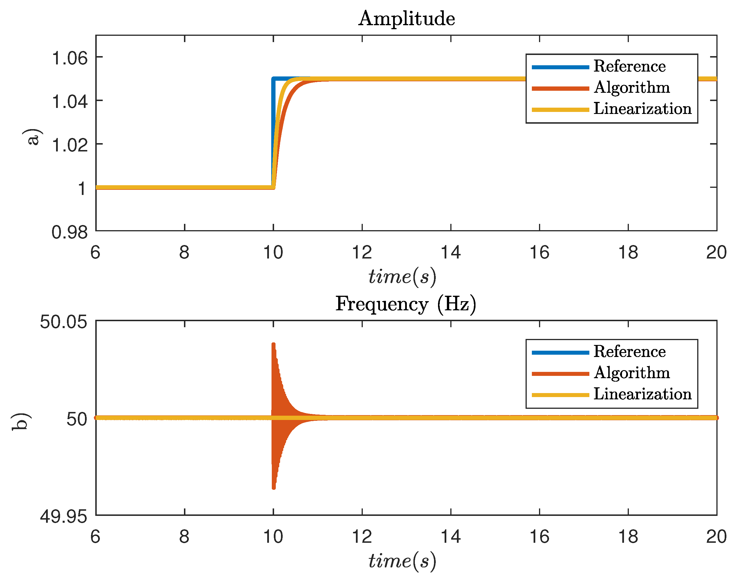
The first test studies the effect of a change in amplitude on the input signal. We take A 0 = 1 and we make a change δ A ^ of 5%. We have plotted, on the Figure 3, the response of the algorithm and that of the linearized system H 1 ( p ) . The two outputs are similar and describe a response of 1er order. On the Figure 3b, the frequencies estimated at the output of the algorithm and the linearized system H 2 ( p ) are plotted. It is noted that a change in the amplitude affects at the same time the estimate of frequency because of the coupling between the amplitude and the frequency in the equations of the algorithm.
The second test shows the effect of changing the input frequency. We choose a frequency f 0 = 50 and we make a change δ f ^ from 0.2 % . The Figure 4 shows the results obtained. The outputs of the algorithm and the linearization have a similar appearance and describe a response of 2ème order. However, we check here the limits of the linearization due to the coupling which is real and not taken into account by the approximation made here.
Although imperfect, the approach adopted here allows us to have an approximate interpretation of the role of the different parameters of the algorithm. The proposed algorithm therefore theoretically makes it possible to obtain the instantaneous frequency of rotation of the machine as well as its mechanical position from a single current measurement. The next step is to sample this rotation frequency as a function of the position with a constant angular sampling step. In the next section, we show that this can be done in real time.

3. Online Re-Sampling

Angular re-sampling is used to overcome the variable speed problem. The hardware solution (HOT) is to implement a sensor providing an electric impulse at every angle increment (constant Δ θ ) and trigging the sampling of the analysis signal. The soft solutions (COT and TOT) use the rotor position and transform the time-dependent vector θ ( t ) into another time-dependent vector with equally spaced position increment using an interpolation algorithm. Several methods allow us to obtain this result [42,43,44,45,46,47]. The previous interpolation algorithms are used in offline mode. In this paper, the same strategy is used but using a new online interpolation method. The corresponding block diagram is shown in Figure 5, this method uses the estimated position θ ^ ( t ) , it detects a constant increase in angle using a quantizer and generates an impulse using a monostable. The new vector of impulses is used to re-sample the time-dependent signal ( s i g n a l ( t ) , Δ t = constant) into a angle-dependent signal ( s i g n a l ( θ ) , Δ θ = constant). The new signal created is stationary and could be studied using classic signal processing tools. In the next section, the identification algorithm and the angular sampling are tested on a test bench.

4. Experimental Results

4.1. Test Bench Description

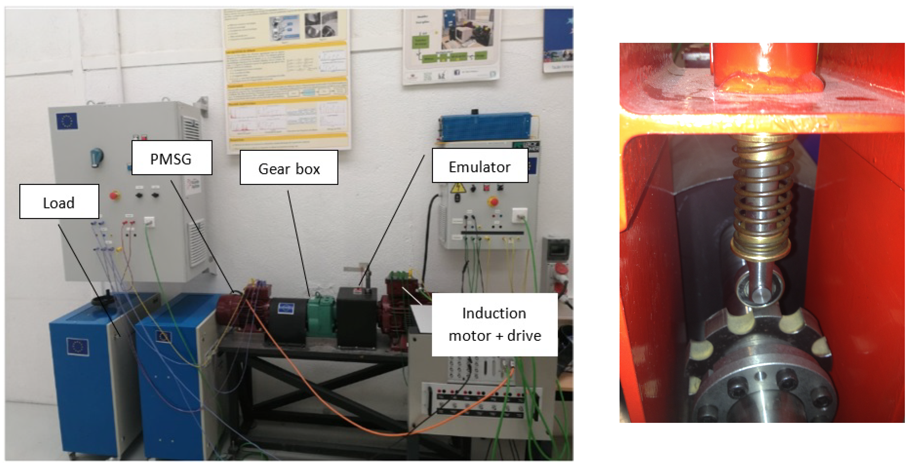
The setup is a wind turbine simulator composed of two 8 KW Permanent Magnet Synchronous Machines. The PMSG (high speed side) is driven by a PMSM (low speed side) through a 4.57 gearbox. The motor is controlled by a Variable speed drive. For the PMSG, the number of pairs of generator poles is P = 4 . A passive load is connected to the PMSG. Position measurement is available on low and high speed sides. Data are collected using the dSPACE-DS1104 acquisition card (dSPACE, Paderborn, Germany). To simulate the fault, a mechanical system designed by our laboratory have been used. The system is mounted on the axis on the low speed side. It contains a roller installed vertically to impact a 9 tooth sprocket, see Figure 6. This system can emulate a fault with frequency of 9 impacts per turn. The force of the impact can be also controlled giving diverse fault strength.

4.2. Test Results

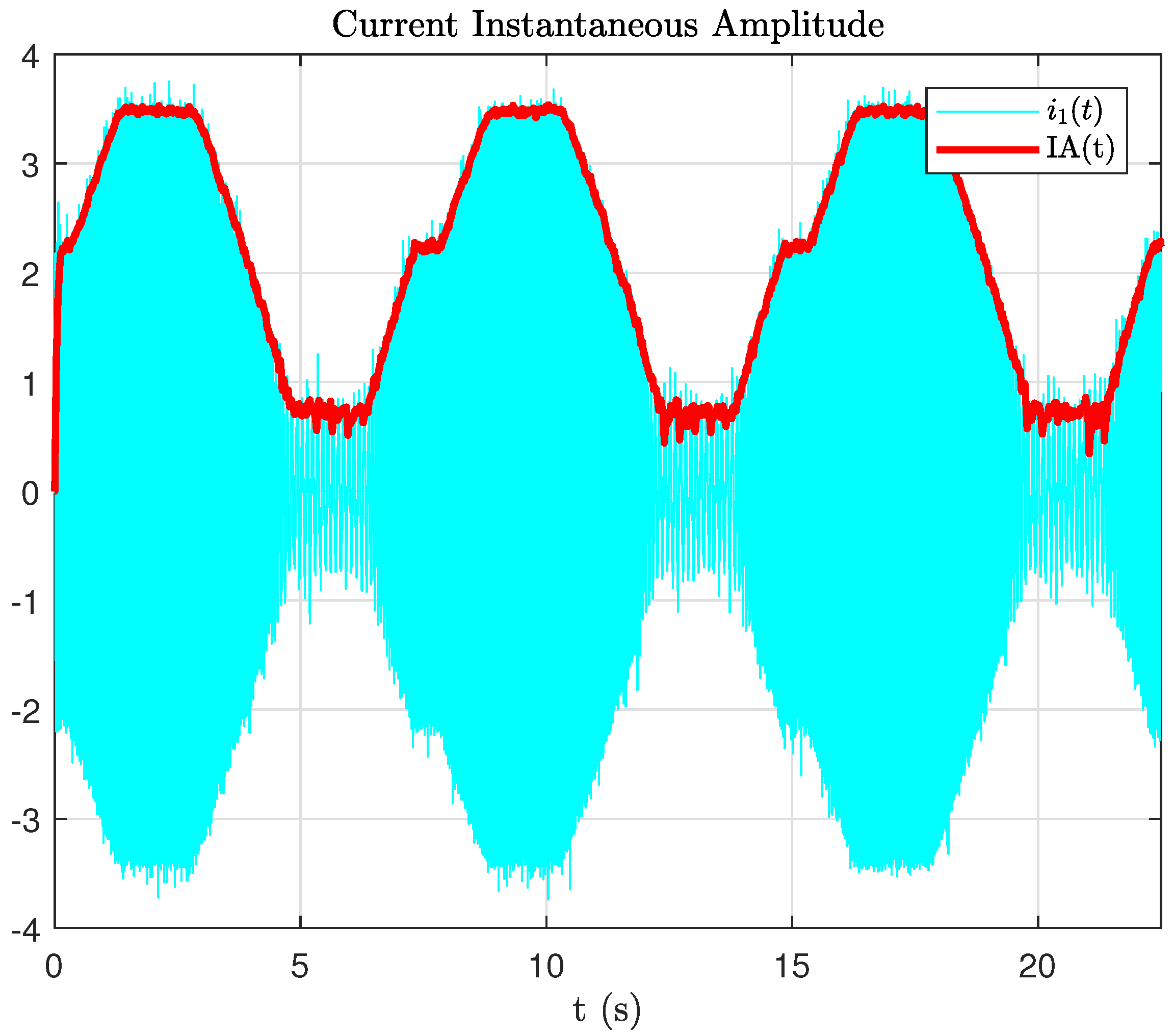
A variable speed test is carried out to test the proposed method. Angular Speed ω ^ ( t ) and position θ ^ ( t ) are estimated by the nonlinear adaptive algorithm using only the current signal i 1 ( t ) . The PMSG runs around a mean frequency of 7 Hz with a constant load torque. The variation margin is between 2 Hz and 12 Hz. The speed cycle period is 7 s corresponding to a frequency of f c y c l e = 0.14 Hz.
The identification algorithm provides the instantaneous amplitude of the current, I A ( t ) , which is a signal of frequency f c y c l e . The parameter m 1 fixes the estimate of I A ( t ) . In this test, it is tuned at m 1 = 20 which corresponds to a cutoff frequency F 1 = 0.5 Hz. Figure 7 shows the current i 1 ( t ) and estimated I A ( t ) . tests are realized with the first record (record 1) with and without defect.
The maximum mechanical frequency is equal to f m = 12 Hz which corresponds to an electric frequency f e = 48 Hz or w e = 300 rad/s. The parameters m 2 and m 3 are fixed respectively at m 2 = 7200 and m 3 = 6.7 × 10 3 which corresponds to a second order filter of proper pulsation ω o = 300 rad/s and a damping coefficient m = 1 . Figure 8 shows shows the estimated frequency compared to the frequency calculated from the position measurement. The machine speed is correctly estimated, but we note the presence of measurement noise on the two signals. We could reduce the bandwidth of the H 2 filter but we risk filtering the component linked to the fault and sought. Figure 9 gives the frequency sampled as a function of the mechanical angle at the output of the block of the Figure 5. The angular sampling step chosen for this test is Δ θ = 0.2 rad.
This signal can now be analyzed by a classical harmonic analysis (FFT). We define an angular sampling frequency equal to g s = 1 Δ θ = 5 rad 1 . The number of samples used to calculate the FFT is N = 8192 so the resolution is Δ g = 5 8192 = 6.1 × 10 4 rad 1 . The spectrum is calculated from 0 to g m a x = g s 2 = 2.5 rad 1 . The unit generally used to represent spectra of angulary sampled signals is not rad 1 but the number of events per revolution. This unit is obtained by multiplying the scale of angular frequencies (g) by 2 π . The spectrum is now represented from 0 to 15.7 ev . t / rev with the resolution Δ g = 3.8 × 10 3 ev . t / rev .
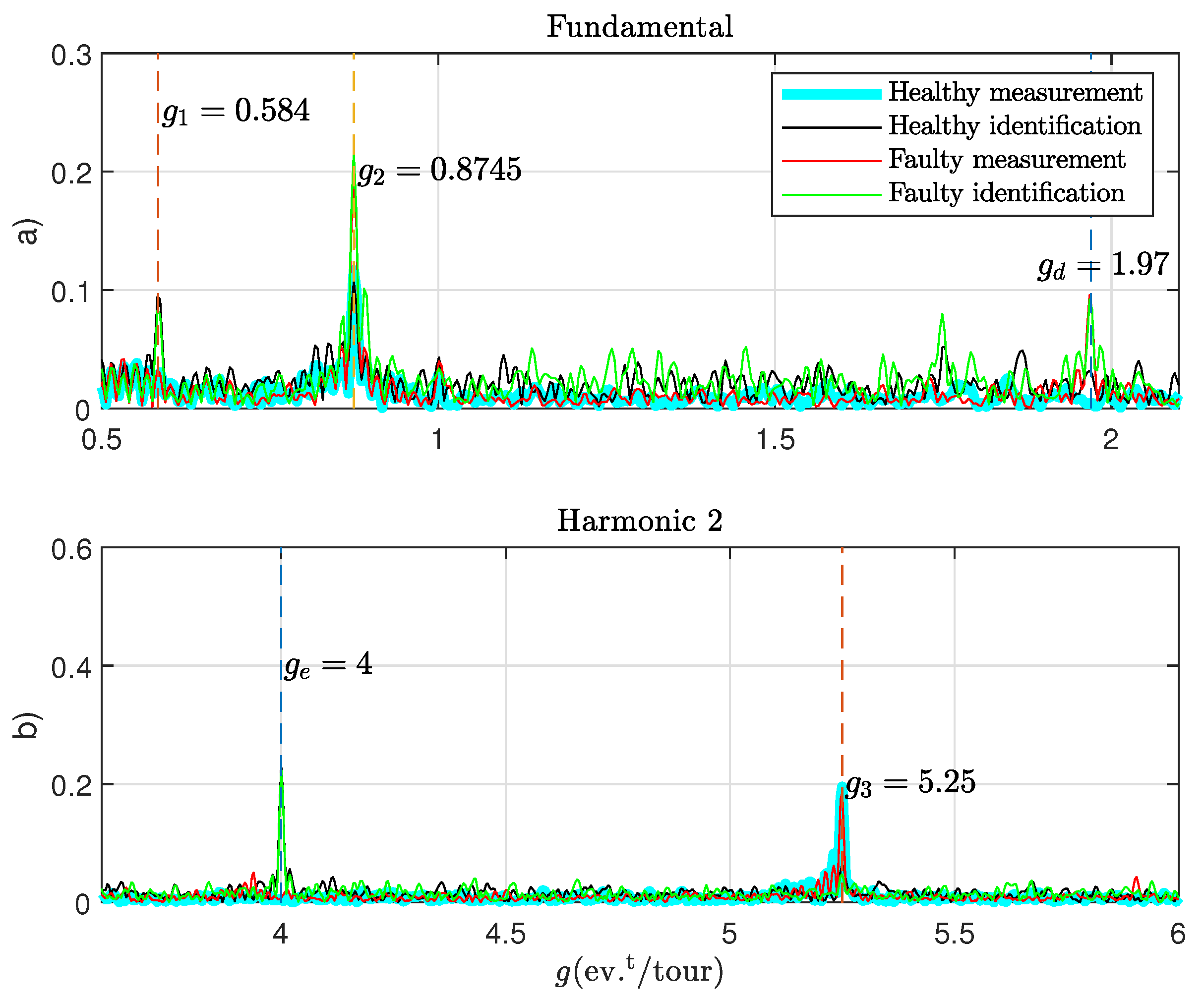
Figure 10 and Figure 11 show the spectra obtained from the signal in Figure 9. The following analysis can be proposed:
  • Components g 2 and g 3 are always detected even in the absence of a fault. They are generated by the gearbox between the emulator and the PMSG.
  • The g 1 component is isolated only by the identification algorithm. It does not correspond to a multiple of the default fundamental g d . It is consequence of aliasing in the angular domain.
  • The component g e relates to the frequency of power supply. It is only detected by the identification algorithm because it uses current as the analysis signal.
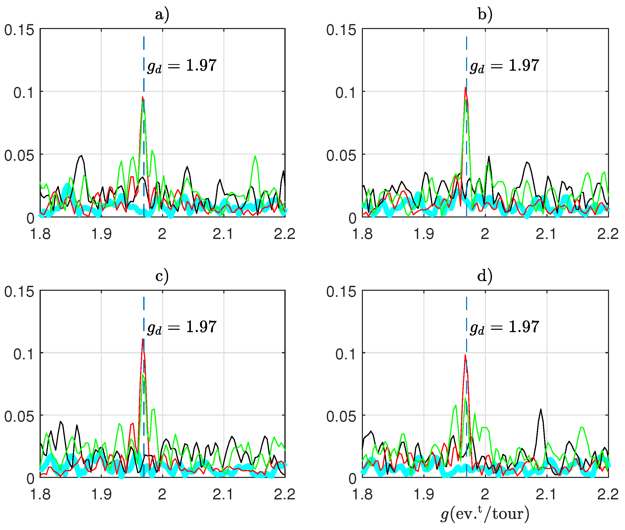
  • In this procedure we are interested in the component corresponding to the impacts generated by the emulator on the generator currents. However, on our test bench, this emulator is placed before the gearbox. So 9 impacts per revolution on the motor side generate, in theory, 9/4.57 = 1.97 impacts per revolution on the generator side. This is what we verify experimentally on the calculated spectra. The fundamental of the defect g d = 1.97 is correctly isolated by the measurement and by the algorithm. By contrast, harmonic 2 is lost in the measurement noise and filtered during identification.
On Figure 12, several records are compared. Healthy spectra (blue and black) are stemmed from record 1. Faulty spectra are calculated from records 2 to 5. For all these tests, the component g d can be detected and its amplitude is comparable with that calculated from measurement.
In this section, we have shown that it is possible to estimate the frequency of rotation and the mechanical position of the generator by identifying the model of the electric current. This information can be used to perform angular sampling and obtain a stationary spectrum whose components no longer vary with speed. With the design chosen for the filter H 2 , only the fundamental of the fault can be detected in the angular spectrum. However, this information is sufficient to carry out an effective detection if it is associated with a statistical approach.

5. Statistical Indicators

5.1. Principle for Constant Speed Functioning

Statistical approach is a robust method requiring a learning phase and making it possible to build a reference for healthy behavior. In [48], a diagnosis strategy was developed using a statistical indicator. The procedure is as follows:
Step 1: choice of signature S f a u l t .
In the case of diagnosis, this can be the amplitude of the spectral component at the frequency of the fault ( f d ) in the estimated mechanical frequency ( f ^ m ).
S f a u l t = f ^ m ( f d )
Step 2: statistical reference.
The machine is considered healthy and N r e f signatures are calculated to build a statistical reference. Once the N r e f samples have been calculated, we can then approximate the statistical distribution that characterizes this behavior. As indicated in [48], the choice of a Gaussian distribution is consistent with the intended application and it suffices to estimate the mean and the standard deviation by the following formulas:
μ ^ r e f = 1 N r e f k = 1 N r e f S f a u l t ( k )
σ ^ r e f = 1 N r e f 1 k = 1 N r e f ( S f a u l t ( k ) μ ^ r e f ) 2
The signature can be improved by making it independent of the machine type used. For this, we define a Reduced Centered (RC) signature defined by:
S f a u l t , R C ( k ) = S f a u l t ( k ) μ ^ r e f σ ^ r e f
Step 3: Automatic alarm threshold
From the S d e f a u l t indicator, an Automatic alarm threshold can be drived in the particular case of a Gaussian distribution law. The alarm threshold used is defined by the relation (22). This definition therefore means that if, for the record n o k , the value of the random variable S d e f a u l t , C R is greater than the threshold t 0.1 % , in theory there is only 0.1% of chance that the system functions in healthy mode.
P ( S f a u l t , R C ( k ) > t 0.1 % ) = 0.001
The above probability can be calculated by the relation:
P ( S f a u l t , R C ( k ) > t ) = 1 Φ ( t )
The value Φ ( t ) cannot be calculated analytically but a table of its numerically obtained values makes it possible to find the desired result. At constant speed, this procedure is very effective and simple to implement. But under variable speed conditions, a single statistical reference is not sufficient for a system whose operating point changes and the creation of the reference must take into account any change in load or speed. The solution proposed in [48] is to create a torque-speed plane segmentation. Each sector represents a working zone of a specific intervals of torque and speed. During the learning phase of the strategy, the electrical system is triggered to work in each sector, then the parameters are calculated and referred to each sector. Data are collected for healthy conditions. After collection, mean and standard deviation are calculated for each sector and a threshold is determined. To detect the fault, the active sector is determined according to actual speed and torque values, then the fault indicator is calculated and compared to data of this active sector And the decision is made. This strategy requires big amount of learning data to cover all zones.

5.2. An Alternative with Order-Tracking

If the data are sampled as a function of the mechanical position, we obtain a stationary spectrum independent of the rotation speed. The torque-speed plane segmentation is no longer necessary. Let’s resume the test presented in the Section 4. We choose to monitor the spectral component located at g d = 1.97 ev . t / rev present in the mechanical frequency estimated by the identification algorithm. The signature is then:
S f a u l t = f ^ m ( g d )
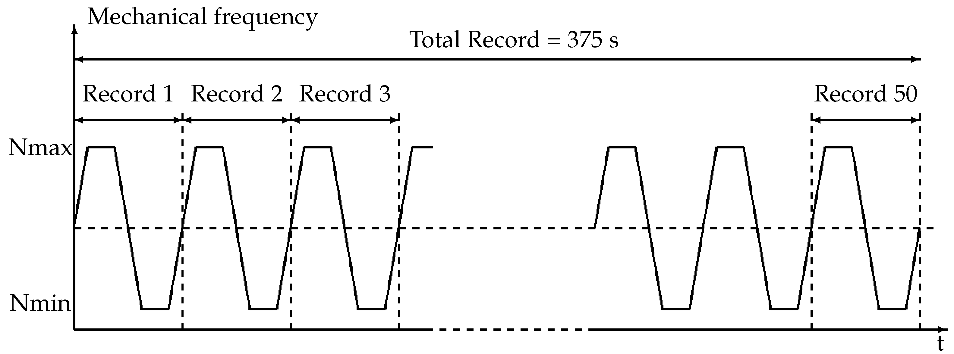
In order to validate the proposed method, a statistical analysis is carried out. The speed cycle of duration 7.5 s is reproduced over a recording time equal to 375 s, i.e., 50 successive records ( N r e f = 50 ). Three different tests were made for different maximum (Nmax) and minimum (Nmin) values of the rotational speed (Figure 13). For each test, the load torque is adjusted to different values corresponding to the currents produced by the generator (Imin and Imax). The numerical values of the different tests are given in the Table 2. Each test is carried out with and without defect.
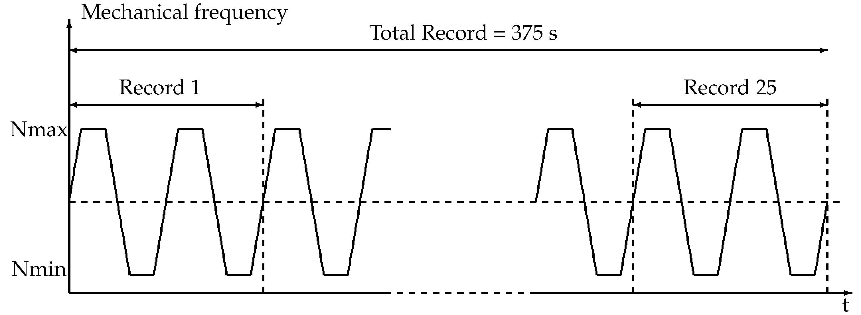
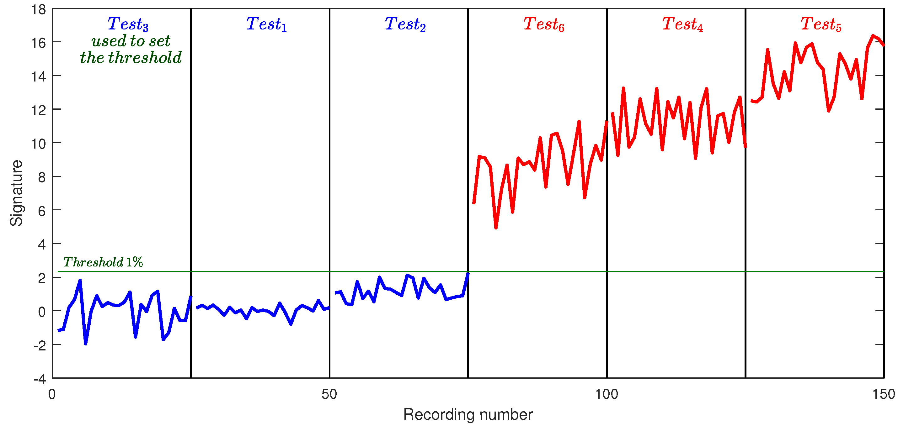
The mean and the standard deviation are calculated using Equations (19) and (20) from Test 3 and used to provide the Reduced Centered signatures defined by Equation (21). By considering (22) and (23) and choosing a probability greater than 1 % , we obtain a threshold equal to t 1 % = 2.33 . The Figure 14 shows the results obtained. It is noted that for the two tests 1 and 2 (healthy) the signatures remain well below the calculated threshold. For the 3 tests with defect, signatures are greater than the chosen threshold. However, in test 6, it is noted that the signature crosses the threshold twice. We note in the Table 2 that for test 3, the generator operates at no load. In this case the current measurements are very noisy. It is possible to solve this problem, by modifying the number of cycles taken into account to calculate the detection threshold. We carry out a new experiment with two cycles of 7.5 s per recording, i.e., a total of 25 recordings (Figure 15). Figure 16 shows the results obtained.

6. Conclusions

The originality of our work lies in the implementation of variable speed order-tracking from only one current measurement, i.e., without position sensor. This approach amounts to considering the current both as an analysis signal (signal containing the fault signature) and as a signal for estimating the mechanical angle. We have shown that, in the particular case of the synchronous machine, this approach was viable and gave satisfactory results. We can rightly consider the synchronous machine as a simple case insofar as the mechanical frequency and the electrical frequency are proportional. It would be interesting to carry out similar work on asynchronous machines where this approach is less obvious due to the slip. In addition, we have implemented a default detection method based on a statistical approach. The classical statistical approach, in the case of variable speed, is relatively complex and requires, as we have seen, to segment the speed/couple plane. The order-tracking approach proposed in this article has made it possible to simplify the implementation of the procedure even if its use seems a priori reduced to repetitive cycles. One avenue of study would be to determine to what extent this approach could be applied in a more general framework.

Author Contributions

E.E., L.R. and S.C. proposed the main idea of the paper; A.A., L.R. and E.E. developed algorithm linearization. L.R. and T.D. developed the online re-sampling system. A.A. and S.C. implemented simulation verification, analyses and experimental tests; A.A. and A.S. developes the statistical approach. The paper was written by A.A., E.E. and L.R., and was revised by S.C., A.S. All the authors were involved in preparing the final version of this manuscript. Besides, this whole work is supervised by A.A., E.E. and L.R. All authors have read and agreed to the published version of the manuscript.

Funding

Research reported in this publication was supported by FEDER Program Poitou-Charentes of the European Union under award number PC158.

Data Availability Statement

Data sharing is not applicable to this article.

Conflicts of Interest

The authors declare no conflict of interest.

References

  1. André, H.; Girardin, F.; Bourdon, A.; Antoni, J.; Rémond, D. Precision of the IAS monitoring system based on the elapsed time method in the spectral domain. Mech. Syst. Signal Process. 2014, 44, 14–30. [Google Scholar] [CrossRef] [Green Version]
  2. Fyfe, K.; Munck, E. Analysis of computed order trackings. Mech. Syst. Signal Process. 1997, 11, 187–205. [Google Scholar] [CrossRef]
  3. Lu, S.; Yan, R.; Liu, Y.; Wang, Q. Tacholess Speed Estimation in Order Tracking: A Review with Application to Rotating Machine Fault Diagnosis. IEEE Trans. Instrum. Meas. 2019, 68, 2315–2332. [Google Scholar] [CrossRef]
  4. Bonnardot, F.; El Badaoui, M.; Randall, R.; Daniere, J.; Guillet, F. Use of the acceleration signal of a gearbox in order to perform angular resampling (with limited speed fluctuation). Mech. Syst. Signal Process. 2005, 19, 766–785. [Google Scholar] [CrossRef]
  5. Wang, Y.; Tang, B.; Meng, L.; Hou, B. Adaptive Estimation of Instantaneous Angular Speed for Wind Turbine Planetary Gearbox Fault Detection. IEEE Access 2019, 7, 49974–49984. [Google Scholar] [CrossRef]
  6. Wang, Y.; Xu, G.; Luo, A.; Liang, L.; Jiang, K. An online tacholess order tracking technique based on generalized demodulation for rolling bearing fault detection. J. Sound Vib. 2016, 367, 233–249. [Google Scholar] [CrossRef]
  7. Zhao, M.; Lin, J.; Xu, X.; Lei, Y. Tacholess Envelope Order Analysis and Its Application to Fault Detection of Rolling Element Bearings with Varying Speeds. Sensors 2013, 13, 10856–10875. [Google Scholar] [CrossRef]
  8. Zhaoa, M.; Lin, J.; Wang, X.; Lei, Y.; Cao, J. A tacho-less order tracking technique for large speed variations. Mech. Syst. Signal Process. 2013, 40, 76–90. [Google Scholar] [CrossRef]
  9. Whu, J.; Zi, Y.; Chen, J.; Zhou, Z. A modified tacho-less order tracking method for the surveillance and diagnosis of machine under sharp speed variation. Mech. Mach. Theory 2018, 128, 508–527. [Google Scholar] [CrossRef]
  10. Wang, Y.; Tse, P.W.; Tang, B.; Qin, Y.; Deng, L.; Huang, T.; Xu, G. Order spectrogram visualization for rolling bearing fault detection under speed variation conditions. Mech. Syst. Signal Process. 2019, 122, 580–596. [Google Scholar] [CrossRef]
  11. Wu, J.; Zi, Y.; Chen, J.; Zhou, Z. Fault diagnosis in speed variation conditions via improved tacholess order tracking technique. Measurement 2019, 137, 604–616. [Google Scholar] [CrossRef]
  12. Wu, J.; Zi, Y.; Chen, J.; Zhou, Z. Tacholess order-tracking approach for wind turbine gearbox fault detection. Front. Mech. Eng. 2017, 12, 427–439. [Google Scholar] [CrossRef]
  13. Niu, J.; Lu, S.; Liu, Y.; Zhao, J.; Wang, Q. Intelligent bearing fault diagnosis based on tacholess order tracking for a variable-speed AC electric machine. IEEE Sens. J. 2018, 19, 1850–1861. [Google Scholar] [CrossRef]
  14. Wang, J.; Peng, Y.; Qiao, W. Current-Aided Order Tracking of Vibration Signals for Bearing Fault Diagnosis of Direct-Drive Wind Turbines. IEEE Trans. Ind. Electron. 2016, 63, 6336–6346. [Google Scholar] [CrossRef]
  15. Wang, J.; Cheng, F.; Qiao, W.; Qu, L. Multiscale Filtering Reconstruction for Wind Turbine Gearbox Fault Diagnosis Under Varying-Speed and Noisy Conditions. IEEE Trans. Ind. Electron. 2018, 65, 4268–4278. [Google Scholar] [CrossRef]
  16. Bossio, J.; Bossio, G.; De Angelo, C. Fault detection for variable-speed wind turbines using vibrations and electrical measurements. In Proceedings of the 2013 Brazilian Power Electronics Conference, Gramado, Brazil, 27–31 October 2013. [Google Scholar]
  17. Pezzani, C.M.; Bossio, J.M.; Castellino, A.M.; Bossio, G.R.; De Angelo, C.H. A PLL-based resampling technique for vibration analysis in variable-speed wind turbines with PMSG: A bearing fault case. Mech. Syst. Signal Process. 2017, 85, 354–366. [Google Scholar] [CrossRef]
  18. Gong, X.; Qiao, W. Bearing fault detection for direct-drive wind turbines via stator current spectrum analysis. In Proceedings of the 2011 IEEE Energy Conversion Congress and Exposition, Phoenix, AZ, USA, 17–22 September 2011. [Google Scholar]
  19. Gong, X.; Qiao, W. Imbalance fault detection of direct-drive wind turbines using generator current signals. IEEE Trans. Energy Convers. 2012, 27, 468–476. [Google Scholar] [CrossRef] [Green Version]
  20. Lu, D.; Gong, X.; Qiao, W. Current-based diagnosis for gear tooth breaks in wind turbine gearboxes. In Proceedings of the 2012 IEEE Energy Conversion Congress and Exposition (ECCE), Raleigh, NC, USA, 15–20 September 2012. [Google Scholar]
  21. Allouche, A.; Etien, E.; Doget, T.; Rambault, L.; Sakout, A.; Cauet, S.; Martin, P. A PLL based mechanical faults detection in PMSM at variable speed. IFAC-PapersOnLine 2018, 51, 1445–1451. [Google Scholar] [CrossRef]
  22. Etien, E.; Rambault, L.; Cauet, S.; Sakout, A. Soft sensor design for mechanical fault detection in PMSM at variable speed. Measurement 2016, 94, 326–332. [Google Scholar] [CrossRef]
  23. Gong, X.; Qiao, W. Bearing fault diagnosis for direct-drive wind turbines via current-demodulated signals. IEEE Trans. Ind. Electron. 2013, 60, 3419–3428. [Google Scholar] [CrossRef] [Green Version]
  24. Lu, S.; Qin, Y.; Hang, J.; Zhang, B.; Wang, Q. Adaptively estimating rotation speed from DC motor current ripple for order tracking and fault diagnosis. IEEE Trans. Instrum. Meas. 2018, 68, 741–753. [Google Scholar] [CrossRef]
  25. Lu, S.; Guo, J.; He, Q.; Liu, F.; Liu, Y.; Zhao, J. A Novel Contactless Angular Resampling Method for Motor Bearing Fault Diagnosis Under Variable Speed. IEEE Trans. Instrum. Meas. 2016, 65, 2538–2550. [Google Scholar] [CrossRef]
  26. Peeters, C.; Leclère, Q.; Antoni, J.; Lindahl, P.; Donnal, J.; Leeb, S.; Helsen, J. Review and comparison of tacholess instantaneous speed estimation methods on experimental vibration data. Mech. Syst. Signal Process. 2019, 129, 407–436. [Google Scholar] [CrossRef]
  27. Li, B.; Zhang, X. A new strategy of instantaneous angular speed extraction and its application to multistage gearbox fault diagnosis. J. Sound Vib. 2017, 396, 340–355. [Google Scholar] [CrossRef]
  28. Prabhakaran, K.; Karthikeyan, A. Electromagnetic Torque-Based Model Reference Adaptive System Speed Estimator for Sensorless Surface Mount Permanent Magnet Synchronous Motor Drive. IEEE Trans. Ind. Electron. 2020, 67, 5936–5947. [Google Scholar] [CrossRef]
  29. Masmoudi, L.; Etien, E.; Moreau, S.; Sakout, A. Amplification of Single Mechanical FaultSignatures Using Full Adaptive PMSM Observer. IEEE Trans. Ind. Electron. 2017, 64, 615–623. [Google Scholar] [CrossRef]
  30. Smith, A.N.; Gadoue, S.M.; Finch, J.W. Improved Rotor Flux Estimation at Low Speeds for Torque MRAS-Based Sensorless Induction Motor Drives. IEEE Trans. Energy Convers. 2016, 31, 270–282. [Google Scholar] [CrossRef] [Green Version]
  31. Comanescu, M. Design and Implementation of a Highly Robust Sensorless Sliding Mode Observer for the Flux Magnitude of the Induction Motor. IEEE Trans. Energy Convers. 2016, 31, 649–657. [Google Scholar] [CrossRef]
  32. Bierhoff, M.H. A General PLL-Type Algorithm for Speed Sensorless Control of Electrical Drives. IEEE Trans. Ind. Electron. 2017, 64, 9253–9260. [Google Scholar] [CrossRef]
  33. Garcia-Calva, T.; Morinigo-Sotelo, D.; Garcia-Perez, A.; Camarena-Martinez, D.; Romero-Troncoso, R. Demodulation Technique for Broken Rotor Bar Detection in Inverter-Fed Induction Motor Under Non-Stationary Conditions. IEEE Trans. Energy Convers. 2019, 34, 1496–1503. [Google Scholar] [CrossRef]
  34. Song, X.; Wang, Z.; Li, S.; Hu, J. Sensorless Speed Estimation of an Inverter-Fed Induction Motor Using the Supply-Side Current. IEEE Trans. Energy Convers. 2018, 34, 1432–1441. [Google Scholar] [CrossRef]
  35. Li, H.; Zhang, X.; Xu, C.; Hong, J. Sensorless Control of IPMSM Using Moving-Average-Filter Based PLL on HF Pulsating Signal Injection Method. IEEE Trans. Energy Convers. 2020, 35, 43–52. [Google Scholar] [CrossRef]
  36. Guan, Q.; Zhang, Y.; Kang, Y.; Guerrero, J.M. Single-Phase Phase-Locked Loop Based on Derivative Elements. IEEE Trans. Power Electron. 2017, 32, 4411–4420. [Google Scholar] [CrossRef]
  37. Golestan, S.; Monfared, M.; Freijedo, F.D.; Guerrero, J.M. Dynamics assessment of advanced single-phase PLL structures. IEEE Trans. Ind. Electron. 2013, 30, 2167–2177. [Google Scholar] [CrossRef]
  38. Ramezani, M.; Golestan, S.; Li, S.; Guerrero, J.M. A simple approach to enhance the performance of complex-coefficient filter-based PLL in grid-connected applications. IEEE Trans. Ind. Electron. 2017, 65, 5081–5085. [Google Scholar] [CrossRef]
  39. Doget, T.; Etien, E.; Rambault, L.; Cauet, S. A PLL-Based Online Estimation of Induction Motor Consumption Without Electrical Measurement. Electronics 2019, 8, 469. [Google Scholar] [CrossRef] [Green Version]
  40. Ziarani, A.; Konrad, A. A method of extraction of nonstationary sinusoids. Signal Process. 2004, 84, 1323–1346. [Google Scholar] [CrossRef]
  41. Siraki, A.G.; Gajjar, C.; Khan, M.A.; Barendse, P.; Pillay, P. An Algorithm for Nonintrusive In Situ Efficiency Estimation of Induction Machines Operating with Unbalanced Supply Conditions. IEEE Trans. Ind. Appl. 2012, 48, 1890–1900. [Google Scholar] [CrossRef] [Green Version]
  42. Sapena-Bano, A.; Pineda-Sanchez, M.; Puche-Panadero, R.; Roger-Folch, J.; Riera-Guasp, M. Harmonic Order Tracking Analysis: A Novel Method for Fault Diagnosis in Induction Machines. IEEE Trans. Energy Convers. 2015, 30, 833–841. [Google Scholar] [CrossRef] [Green Version]
  43. Sapena-Bano, A.; Burriel-Valencia, J.; Pineda-Sanchez, M.; Puche-Panadero, R.; Riera-Guasp, M. The Harmonic Order Tracking Analysis Method for the Fault Diagnosis in Induction Motors Under Time-Varying Conditions. IEEE Trans. Energy Convers. 2017, 32, 244–256. [Google Scholar] [CrossRef] [Green Version]
  44. Cheng, F.; Wei, C.; Qu, J.; Qiao, W. Fault diagnosis of wind turbine gearbox using DFIG stator current analysis. In Proceedings of the 2016 IEEE Energy Conversion Congress and Exposition (ECCE), Milwaukee, WI, USA, 18–22 September 2016. [Google Scholar]
  45. Blough, J. A survey of DSP methods for rotating machinery analysis, what is needed, what is available. J. Sound Vib. 2003, 262, 707–720. [Google Scholar] [CrossRef]
  46. Lee, J.; Hong, J.; Nam, K.; Ortega, R.; Praly, L.; Astolfi, A. Sensorless Control of Surface-Mount Permanent-Magnet Synchronous Motors Based on a Nonlinear Observer. IEEE Trans. Power Electron. 2010, 25, 290–297. [Google Scholar]
  47. Gong, X.; Qiao, W. Current-based mechanical fault detection for direct-drive wind turbines via synchronous sampling and impulse detection. IEEE Trans. Ind. Electron. 2015, 62, 1693–1702. [Google Scholar] [CrossRef]
  48. Fournier, E.; Picot, A.; Régnier, J.; Maussion, P.; TientcheuYamdeu, M.; Andréjak, J. A generic diagnosis protocol for the monitoring of induction motors based on multiple statistical references in the torque-speed plane. In Proceedings of the IECON 2014—40th Annual Conference of the IEEE Industrial Electronics Society, Dallas, TX, USA, 29 October–1 November 2014. [Google Scholar]
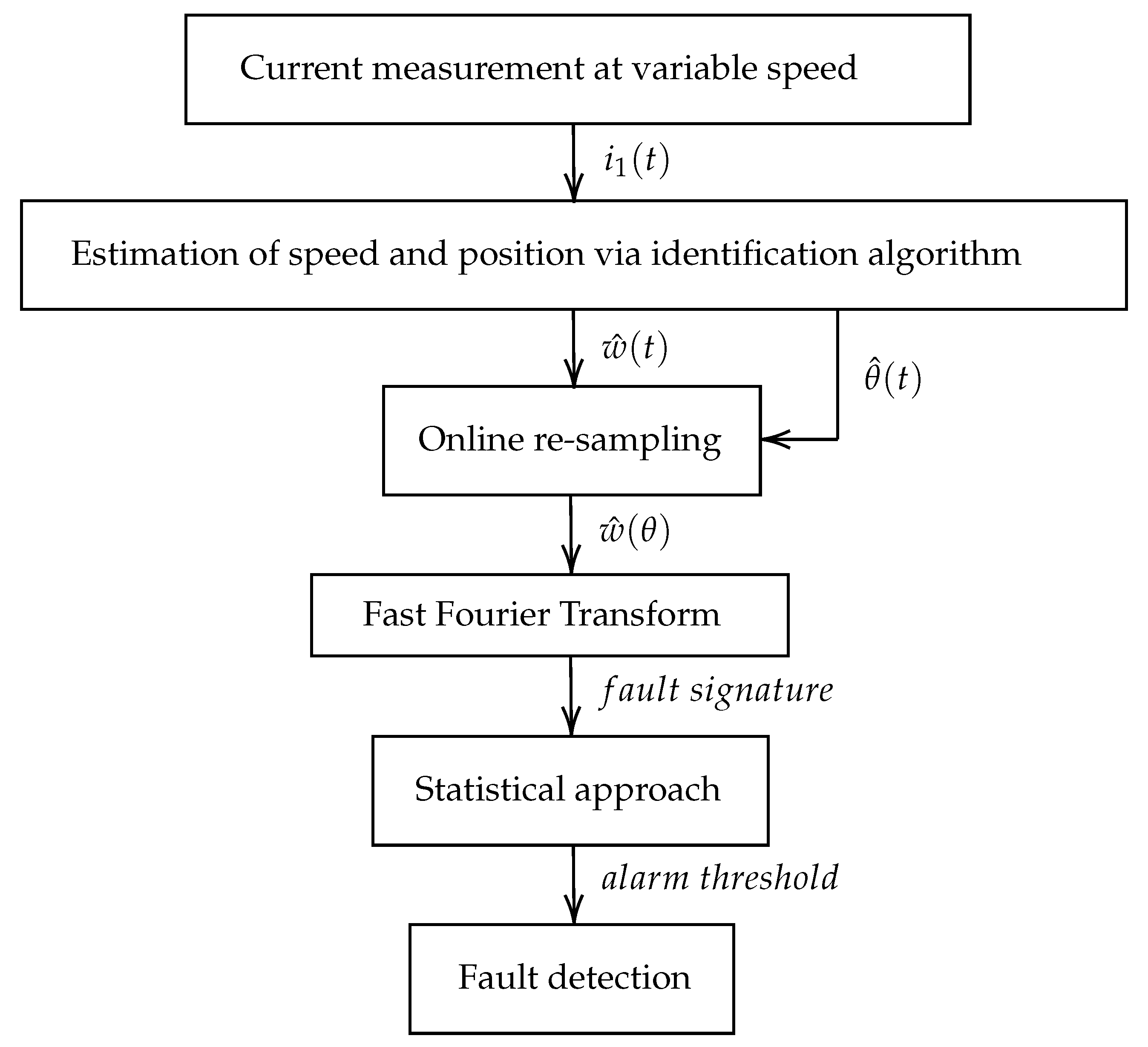
Figure 1. Flowchart of the proposed method.
Electronics 10 00418 g001
Figure 2. Block diagram of the nonlinear adaptive algorithm.
Electronics 10 00418 g002
Figure 3. Amplitude tracking. (a) amplitude step; (b) frequency output of the algorithm.
Electronics 10 00418 g003
Figure 4. Frequency tracking. (a) amplitude output of the algorithm, (b) frequency step.
Electronics 10 00418 g004
Figure 5. Block diagram of the online re-sampling.
Electronics 10 00418 g005
Figure 6. Test bench and fault emulator.
Electronics 10 00418 g006
Figure 7. Phase current i 1 ( t ) and I A ( t ) , m 1 = 20 .
Electronics 10 00418 g007
Figure 8. Generator mechanical frequencies, m 2 = 7200 , m 3 = 6.7 × 10 3 .
Electronics 10 00418 g008
Figure 9. Frequency as a function of mechanical position.
Electronics 10 00418 g009
Figure 10. Angular spectrum of mechanical frequency. (a) between 0.5 and 2 ev . t / rev , (b) between 0 and 6 ev . t / rev .
Electronics 10 00418 g010
Figure 11. Zooms of angular spectrum of mechanical frequency around fault components. (a) between 1.8 and 2.2 ev . t / rev , (b) between 3.8 and 4.2 ev . t / rev .
Electronics 10 00418 g011
Figure 12. Comparison for different records. (a) to (d) respectively records 2 to 5.
Electronics 10 00418 g012
Figure 13. Speed profile for experimental tests.
Electronics 10 00418 g013
Figure 14. Signatures, 1 period, N r e f = 50 .
Electronics 10 00418 g014
Figure 15. Speed profile for experimental tests.
Electronics 10 00418 g015
Figure 16. Signatures, 2 period, N r e f = 25 .
Electronics 10 00418 g016
Table 1. Tacholess Order Tracking (TOT) and applications.
Ref.Analysed SignalAngle Estimate
[5,6,7,8,9,10,11,12]vibrationvibration
[13,14,15]vibrationcurrent
[16]vibrationcurrents/voltages + observer
[17]vibrationvoltages
[18,19,20]currentcurrent
[21] I F current
[22] I F currents/voltages + observer
[23] I A and I F current
[24]soundcurrent
[25]soundvideo
Table 2. Tests setup.
TestNmin (rpm)Nmax (rpm)Imin (A)Imax (A)Default
Test 115045026No
Test 245075069.5No
Test 315075014No
Test 415045026Yes
Test 545075069.5Yes
Test 615075014Yes
Publisher’s Note: MDPI stays neutral with regard to jurisdictional claims in published maps and institutional affiliations.