Elastic Downsampling: An Adaptive Downsampling Technique to Preserve Image Quality

Abstract

This paper presents a new adaptive downsampling technique called elastic downsampling, which enables high compression rates while preserving the image quality. Adaptive downsampling techniques are based on the idea that image tiles can use different sampling rates depending on the amount of information conveyed by each block. However, current approaches suffer from blocking effects and artifacts that hinder the user experience. To bridge this gap, elastic downsampling relies on a Perceptual Relevance analysis that assigns sampling rates to the corners of blocks. The novel metric used for this analysis is based on the luminance fluctuations of an image region. This allows a gradual transition of the sampling rate within tiles, both horizontally and vertically. As a result, the block artifacts are removed and fine details are preserved. Experimental results (using the Kodak and USC Miscelanea image datasets) show a PSNR improvement of up to 15 dB and a superior SSIM (Structural Similarity) when compared with other techniques. More importantly, the algorithms involved are computationally cheap, so it is feasible to implement them in low-cost devices. The proposed technique has been successfully implemented using graphics processors (GPU) and low-power embedded systems (Raspberry Pi) as target platforms.

1. Introduction

Downsampling techniques are widely used in signal processing and transmission as they save computation time, storage, and bandwidth. Image reconstruction using a sampled data source can be applied in image storage and transmission but also for frame sampling reduction, where intermediate frames must be reconstructed (e.g., slow motion software or tomographic images) [1].

Downsampling is generally preceded by an antialiasing filter to reduce undesired noise, i.e., each resulting sample corresponds to the average of a certain number of original samples (sample rate). This process is known as “decimation”. The antialias filtering prior to downsampling enforces the Nyquist criterion at the downsampling stage, allowing bandlimited signal reconstruction.

The complementary mechanisms, called interpolation, scaling or upsampling, intends to create intermediate samples from the available ones. There are several interpolation techniques with different quality results and different computational costs [2,3].

In contrast to downsampling algorithms, which equally decrease the quality of the whole original image, adaptive downsampling algorithms aim to assign higher sampling rates to complex or detailed areas [4]. There are several known methods to assign an adaptive sampling rate to the different blocks of an image based on frequency analysis [5] or space (luminance) analysis [6]. This set of sampling rates constitutes the sampling rate vector.

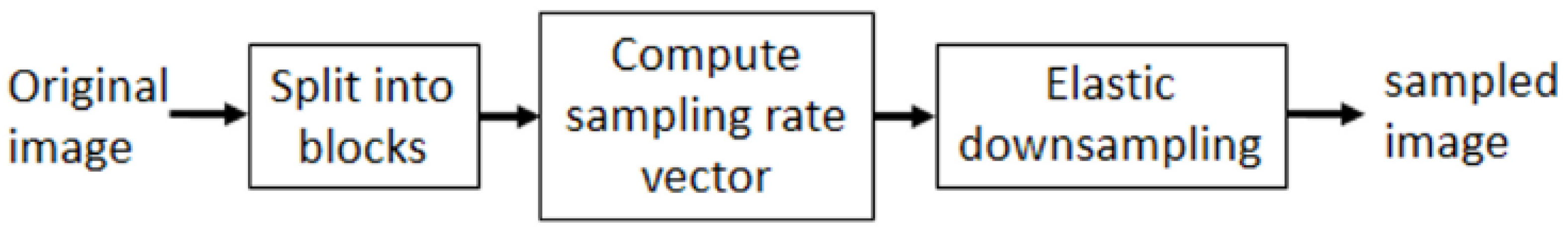
Existing block-based adaptive downsampling methods [6] share a common drawback: the change of sample rate at the frontiers between adjacent blocks produces undesirable blocking effects and artifacts. Solving this problem is the main motivation of this work: to propose a novel elastic downsampling technique that features no sample-rate discontinuities and a metric to evaluate the relevance of an image region to assign a sampling rate to each block’s corner (Figure 1).

The computation of the sampling rate vector is based on a “Perceptual Relevance” metric, which relies on a luminance analysis to determine the suitable sampling rate for each block corner. Once the sampling rate vector has been computed, the elastic downsampling process can be performed. This downsampling technique allows the adjustment of the sampling rate inside a block by defining an initial and a final sampling rate values. This mechanism avoids blocking effects by keeping a continuous linear sampling rate, smoothly evolving across the whole image.

This paper is organized as follows. Section 2 surveys the most relevant work related to the proposed algorithm. Section 3 briefly introduces elastic downsampling and describes the Perceptual Relevance (PR) metric. Section 4 details the elastic downsampling algorithm that uses this metric. Section 5 introduces the elastic interpolation mechanism. Section 6 shows the main results that have been obtained in the evaluation stage of the algorithm. Section 7 discusses the benefits and limitations of the proposed technique and applies the algorithm to a codec designed for real-time video, showing its validity. Finally, Section 8 summarizes the main contributions of this paper and outlines future lines of work.

2. Related Work

The goal of all existing downsampling methods is to reduce the original information while damaging the quality as little as possible. In the literature, most of the adaptive downsampling techniques can be classified into two types:

• Those applied block by block at different sample rates [4,6], using a sampling rate vector.
• Those applied to the whole frame at a fixed sampling rate, by balancing the distortion composition (coding distortion and downsampling distortion) in order to reach an optimal total distortion value [7,8]. For example, in [8], the proposed method is focused in filtering the image before sampling, using an adapted-content kernel at each image position, allowing for a higher quality subsequent subsampling.

There is another approach that looks at the problem the other way around, trying to maximize the perceived quality of a final image built from an original picture with little information. This approach focuses on choosing the most effective interpolation method [9] to extract the maximum quality from the given samples and has been particularly well developed for specific image types created by computer (“pixel-art”) [10,11]. These interpolation techniques can be combined with optimized downsampling methods in order to improve the quality even further.

Going back to the downsampling methods, all of them follow these two main approaches to compute the sampling vector:

(a)

Sample rate based on spatial analysis

(b)

Sample rate based on frequency analysis

2.1. Adaptive Sample Rate Based on Spatial Analysis

These methods compute the sampling rate vector by processing the image at the spatial domain. In [2], the authors use this approach with the standard deviation of the light intensity of each image block. The results show that the proposed methods provide a better Peak Signal-to-Noise Ratio (PSNR) than the other compared methods. However, some blocking artifacts may appear in the frontier between two consecutive downsampled blocks as they may have different sampling rates. In [12], the authors propose to compute a Just-Noticeable Difference (JND) luminance activity threshold to make the downsampling decision, previous to image compression, improving the final bitrate.

2.2. Adaptive Sample Rate Based on Frequency Analysis

These methods process the image at the frequency domain to compute the sampling rate vector. This approach is studied in [13], with a method based on image frequency statistics and their correlation with the optimal downsampling factor. In [14], the authors propose a codec which adaptively selects smooth regions of the original image to downsample according to Discrete Cosine Transform (DCT) coefficients and the current coding bit rate. In [15], the authors present a thresholding technique for image downsampling based on the Discrete Wavelet Transform (DWT) and a Genetic Algorithm (GA). The proposed method is divided into four different phases: preprocessing, DWT, soft thresholding, and GA. The preprocessing phase converts from RGB color space to greyscale and reduces the motion blur by using a motion filter. Then, the image is segmented into blocks and the DWT is applied to them to reduce the image size. The soft thresholding mechanism is used for reducing the background in the image. Finally, a GA is applied for identifying the number of thresholds and the threshold value. The downsampled image is obtained by comparing block similarities by using Euclidean distances and removing all the similar blocks. The results show improvements compared to an existing method called Interpolation-Dependent Image Downsampling (IDID) [16].

In [17], the authors propose a method to adaptively determine a downsampling mode and a quantization mode of each image macroblock using the ratio distortion optimization method, improving compression at low bit rates.

2.3. Limitations of the Current Downsampling Methods

All of the downsampling methods in the literature that rely on a sampling rate vector suffer from the same problem: the change of the sample rate at the frontiers between adjacent blocks, which may produce undesirable blocking effects and visual artifacts. This effect becomes more noticeable when an object inside the image appears in several adjacent blocks that have been sampled at different sample rates. Overcoming this undesirable effect is one of the reasons behind the elastic downsampling method proposed in this paper.

3. Proposed Perceptual Relevance Metric

This section briefly introduces the whole elastic downsampling process and then details the Perceptual Relevance metric that this process uses.

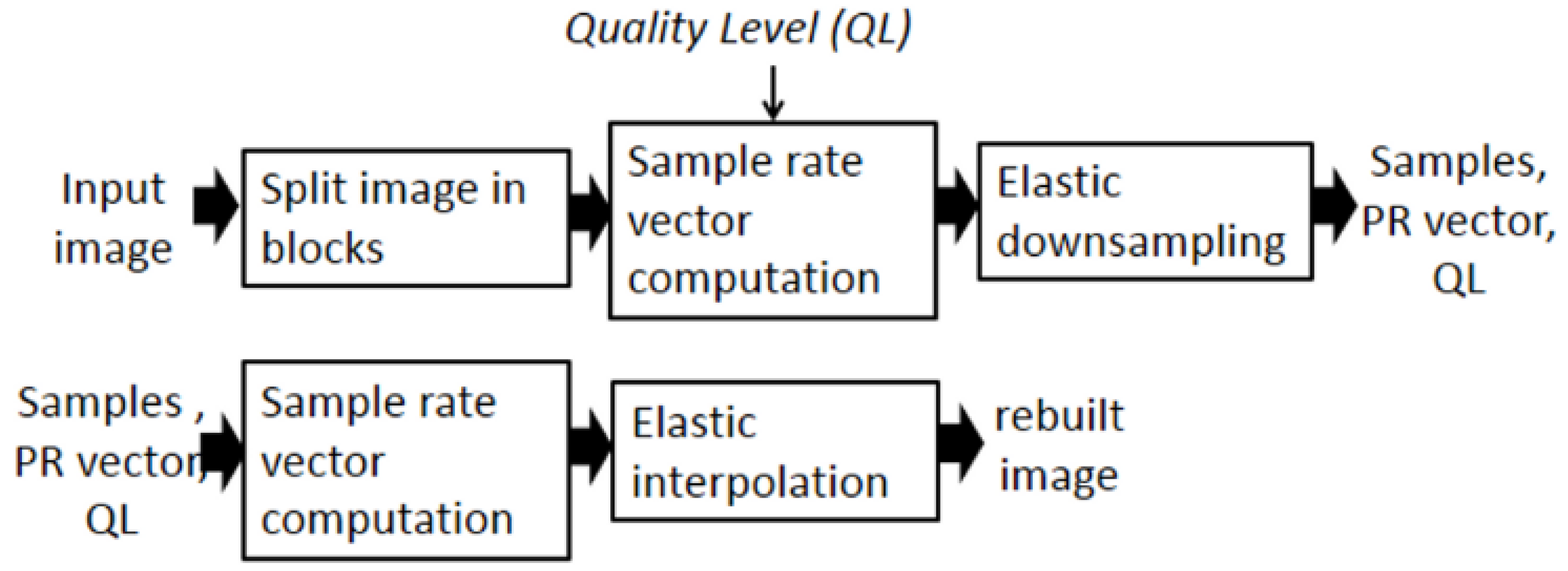
Figure 2 summarizes the proposed elastic downsampling and its corresponding elastic interpolation process. For the downsampling process, the original image is first split into blocks. In the sample rate vector computation, the Perceptual Relevance (PR) is evaluated at each corner of each block, resulting in a list of value pairs $(P{R}_x,P{R}_y)$. This list is later translated into sampling rate values which will evolve from corner to corner at the elastic sampling stage. The reverse procedure considers the resulting samples and the PR list and applies an elastic interpolation process to recover the original image.

Given a desired compression level (defined by “Quality Level” parameter), the evaluation of an image block’s interest must provide a metric, which may be translated into a sampling rate. Since this is a measurement of the block’s perceptual relevance, it can be used as a criterion to define the number of samples used to encode each block. Therefore, we propose a novel Perceptual Relevance metric of an image block which may be defined as a measure of the importance of the block regarding the complete image, as perceived by a human viewer [18].

Luminance fluctuations in both vertical and horizontal directions can be used as an estimator of the PR in an image block, since a change in the luminance gradient reveals edges or image details. Therefore, the number of such changes and their corresponding sizes are proposed as PR estimators. The processing is carried out as follows:

• The image is divided into blocks.
• The PR metric is calculated at each block corner. To achieve this, an imaginary block grid (Figure 3), where the center of each block matches with the block corners of the elastic grid, must be created.
• The PR metrics are modified to lie within two thresholds (histogram expansion) and finally quantized and translated to sample rate values.

3.1. PR Metrics Computation

For the PR metrics calculation, the luminance gradient changes are measured, to enable the downsampling of each block with a greater or lesser intensity. Since a PR value is related to its interpolation capability, a block with a higher PR value will need more samples to be rebuilt than other with lower PR information. For example, a white block can be interpolated using only one sample while a block containing a more complex object, such as an animal eye, would need more samples to be reconstructed.

It is possible to measure the interpolation capability of an image block by using the sign changes of the luminance gradient and their size. The PR must be computed in both directions, horizontal and vertical, resulting in a couple $(P{R}_x,P{R}_y)$ per corner, which are normalized to the range $[0,1]$.

The computation is performed scanline by scanline. For each scanline, a luminance gradient $g_i$ is computed as the logarithmical difference of luminance between two consecutive pixels Equation (1), and it is quantized to an integer value within the interval $[0,4]$. The $-2$ offset in the Equation (1) sets 8 as the minimum detectable luminance difference in $g_i$ (the luminance gradient), and $l_i$ is the luminance signal value at pixel i.

$$\begin{array}{ccc}\hfill g_i=\lfloor lo{g}_2\left(\left|l_i-l_{i-1}\right|\right)-2\rfloor ,& & \mathrm{if}{g}_i>4\mathrm{then}{g}_i=4\hfill \end{array}$$

(1)

As shown in Figure 3, the PR metric is calculated in the corner of each block. To perform this operation, luminance values inside an imaginary block are analyzed separately for the two coordinates using the following rules:

• For each scan, and for each pixel, the value of the $g_i$ value is cumulated and the counter of $g_i$ values greater than 0 is registered into $C_x$ (horizontal scans) or $C_y$ (vertical scans).
• After all scans are processed, the resulting cumulated value of $g_i$ is divided by the counter multiplied by 4 (the maximum value of each $g_i$). The resulting value is within the range $[0,1]$ (see Equations (2) and (3)).

  $$\begin{array}{ccc}\hfill P{R}_x& =& \frac{{\sum }_{i=1}^{C_x}{g}_i}{C_x·4}\hfill \end{array}$$

  (2)

  $$\begin{array}{ccc}\hfill P{R}_y& =& \frac{{\sum }_{i=1}^{C_y}{g}_i}{C_y·4}\hfill \end{array}$$

  (3)

There are some imaginary blocks that cover the image only partially (Figure 3). In such cases, only the pixels inside the image area are considered for the PR metric computation.

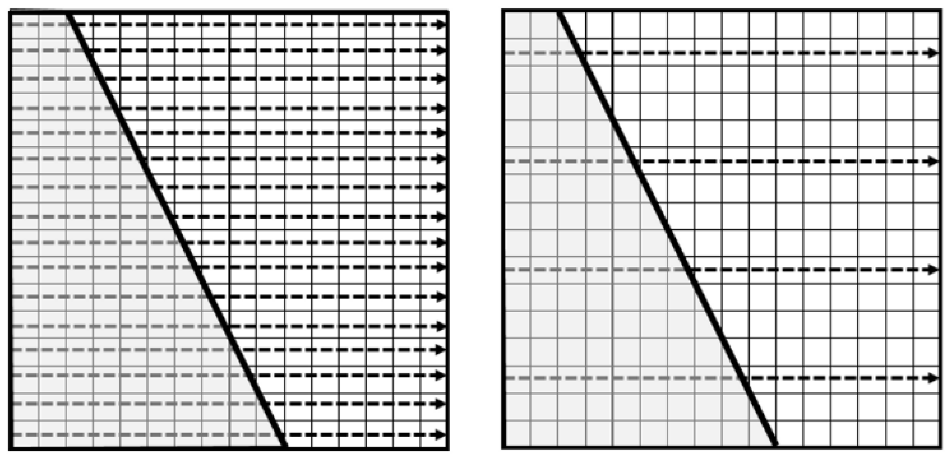
The aforementioned PR formula considers all block scanlines, based on the average size of their luminance changes, and it is independent of the number of such changes. Based on this reasoning, a performance optimization may be possible by reducing the number of analyzed scanlines. Instead of processing all scanlines of a block to compute the PR, a subset of them is enough to intersect the edges of the shapes included inside it and obtain an equivalent measurement. Figure 4 illustrate this point, since the same diagonal with a smaller number of processed scanlines produces similar results.

Algorithm 1 shows the pseudocode for the computation of $P{R}_x$.

Algorithm 1$P{R}_x$ computation.

1: for each scan line in block do  2:     for each x coordinate do  3:         $A=pixel\left[x\right]$  4:         $B=pixel[x-1]$  5:         $gradient=\lfloor (lo{g}_2\left(\right|B-A\left|\right)-2)\rfloor$  6:         if $gradient>0$ then  7:            $counter++$  8:            if $gradient>4$ then  9:                $gradient=4$ 10:            end if 11:            $acum=acum+gradient$ 12:         end if 13:     end for 14: end for 15: $P{R}_x=acum/(counter·4)$

3.2. PR Limits and Histogram Expansion

PR saturates in cases where sensory information is very high (or noisy). This means that the perception does not change whether the information increases or decreases. In this paper, the PR saturation threshold ($P{R}_{max}$) is defined as the value from which perceptual information hardly varies. If this threshold was not considered, the noise would be more protected than the useful information, because higher PR values will be transformed into higher sample rates. By the same reasoning, a $P{R}_{min}$ threshold should also be considered, to avoid differentiation among very low values of PR.

Once these two thresholds have been established, PR metrics fall within the interval $[P{R}_{min},P{R}_{max}]$. Considering that each block’s corner of the elastic grid has a pair of PR values $(P{R}_x,P{R}_y)$ to be saved into the image file, these metrics must be quantified into PR levels before the save operation. However, if the PR histogram is very compact, i.e., PR values are very similar to each other; it may happen that all values are quantized to the same PR level. In this situation, it would not be possible to perform a suitable image downsampling. To avoid this problem, a PR histogram expansion from a minimum PR value ($P{R}_{min}$) to a maximum PR value ($P{R}_{max}$) must be applied.

• $P{R}_{min}$: PR values lower than $0.125$ correspond to small signal fluctuations. It means that this is a soft area of the image. For this reason, they will be transformed in 0.
• $P{R}_{max}$: PR saturation threshold was established at $0.5$. Thus, PR values above $0.5$ will be transformed in 1. This threshold avoids protecting more the noise than the real edges of the image.

Before the expansion, the PR range lies within $[P{R}_{min}=0.125,P{R}_{max}=0.5]$. The formula applied to perform the PR histogram expansion is defined in Equation (4). After the PR histogram expansion, the PR range is $[0,1]$. In Equation (4), $P{R}_{init}$ is the PR value before the PR histogram expansion, and $P{R}_{end}$ is the PR value after the PR histogram expansion.

$$\begin{array}{ccc}\hfill P{R}_{end}& =& \frac{P{R}_{init}-P{R}_{min}}{P{R}_{max}-P{R}_{min}}\hfill \end{array}$$

(4)

The values for PRmin and PRmax were determined experimentally. The computation of pure noise produced a PR value around 0.8, while images from the USC-SIPI gallery [19] does not exceed $0.5$. In addition, the minimum PR value for very soft (but not null) areas found in that photo gallery is $0.125$.

3.3. PR Quantization

The next step is the PR quantization, where different PR values are translated into five different quant values (see

Table 1. PR quantization.

Quant Interval	PR Quantised Value	Value Meaning
$[0.75,1.0]$	$1.0$	Corners whose PR value was limited to the PR saturation threshold
$[0.5,0.75)$	$0.5$	High relevance
$[0.25,0.5)$	$0.25$	Medium relevance
$[0.125,0.25)$	$0.125$	Low relevance
$[0.0,0.125)$	$0.0$	Blocks without relevance

). This quantization aims to reduce the amount of information consumed by PR values for image transmission or storage. While the number of quants can be configured, this paper proposes five different values.

Quantized PR values will be translated into sample rates. A more accurate PR value would provide more quality. However, a higher accuracy implies more information, and the benefits of elastic downsampling would be canceled by the space taken by the PR data.

Table 1 shows that the quantization follows a nonlinear distribution. The underlying rationale is that, in common general photographic images, the computation of the sample rate based on nonlinear quants produces better results than linear distribution.

3.4. Translation of PR into a Sample Rate

Thanks to the PR metric, it is possible to assign different sampling rates to each block corner. Image samples are taken in accordance with the sampling rate evolution from corner to corner. The result is an image that has been downsampled in an elastic way.

First, the maximum compression or maximum sampling rate value ($S_{max}$) must be defined. Given an image width ($imag{e}_{width}$) and the number of blocks $N_{block}$ in which the image is going to be divided at the larger side (width or height), the block side length (l) is computed see Equation (5). The maximum sampling rate Equation (6) is related to the original image size and the number of blocks in which it was divided. The downsampled size of the block side is notated as $l^{{}^{\prime }}$ Equation (7) and the minimum size for each downsampled block is $2\times 2$ ( value of $l_{min}^{{}^{\prime }}$ is 2) because each corner may have a different sampling rate value, i.e., at least one pixel for each corner (4 pixels per block) must be preserved. For example, in common video formats, the larger side is located on the horizontal axis.

$$\begin{array}{ccc}\hfill l& =& \frac{image\text{\_}width}{N_{block}}\hfill \end{array}$$

(5)

$$\begin{array}{ccc}\hfill S_{max}& =& l/2\hfill \end{array}$$

(6)

Taking into account the aforementioned equations and an eligible compression factor (CF) between 0 and 1, the formula relating both concepts is shown in Equation (8), where the sample rate (S) expression is shown.

$$\begin{array}{ccc}\hfill l^{\prime }& =& l_{min}^{{}^{\prime }}+(l-l_{min}^{{}^{\prime }})·PR\hfill \end{array}$$

(7)

$$\begin{array}{ccc}\hfill S& =& \frac{l}{l^{{}^{\prime }}}=\frac{S_{max}}{1+(S_{max}-1)·PR}·CF\hfill \end{array}$$

(8)

Some examples of the maximum compression ratios and $S_{max}$ for different image sizes are shown in

Table 2. $S_{max}$ and Max compression ratio for different image sizes divided into 32 blocks widthwise.

Image Size	Blocks	${\mathit{S}}_{\mathbf{max}}$	Max Compression Ratio
$512\times 512$	$32\times 32$	8	1:64
$640\times 480$	$32\times 24$	10	1:100
$800\times 600$	$32\times 24$	12	1:156
$1024\times 768$	$32\times 24$	16	1:256
$1280\times 1024$	$32\times 26$	20	1:393

. The number of blocks that have been considered is $Nblock=32$.

Elastic downsampling does not use a fixed block size; instead, it considers a grid with a fixed number of blocks with variable size. This approach results in different block sizes for different image sizes. Our experiments have been conducted using a value of $N_{blocks}=32$ for the large side of the image. This value is configurable, but a higher number produces large vectors of PR, thus consuming more information. The minimum possible value is 1, considering the entire image as a single block. As could be expected, this verge case features a poor adaptive downsampling effectiveness.

4. Proposed Elastic Downsampling Method

This section details the elastic downsampling method briefly introduced in Section 3 (Figure 2).

Depending on the desired quality level (QL), the translation of PR values into sampling ratio values will be more or less destructive. Nevertheless, higher PR values will always be translated into higher sampling ratio values, thus preserving better quality in relevant areas.

In the proposed method, samples are taken with different sampling ratios across the same block. More concretely, this ratio varies from corner to corner, but adjacent blocks will have the same sampling ratio at their common frontier to prevent blocking effects. This variable sampling ratio is represented by the letter “S” in the formulas. For instance, a value $S=4$ means that one sample represents four original pixels.

As it can be inferred, S cannot be less than 1, and it can have different values at each corner of each block and in each dimension $(S_x,S_y$).

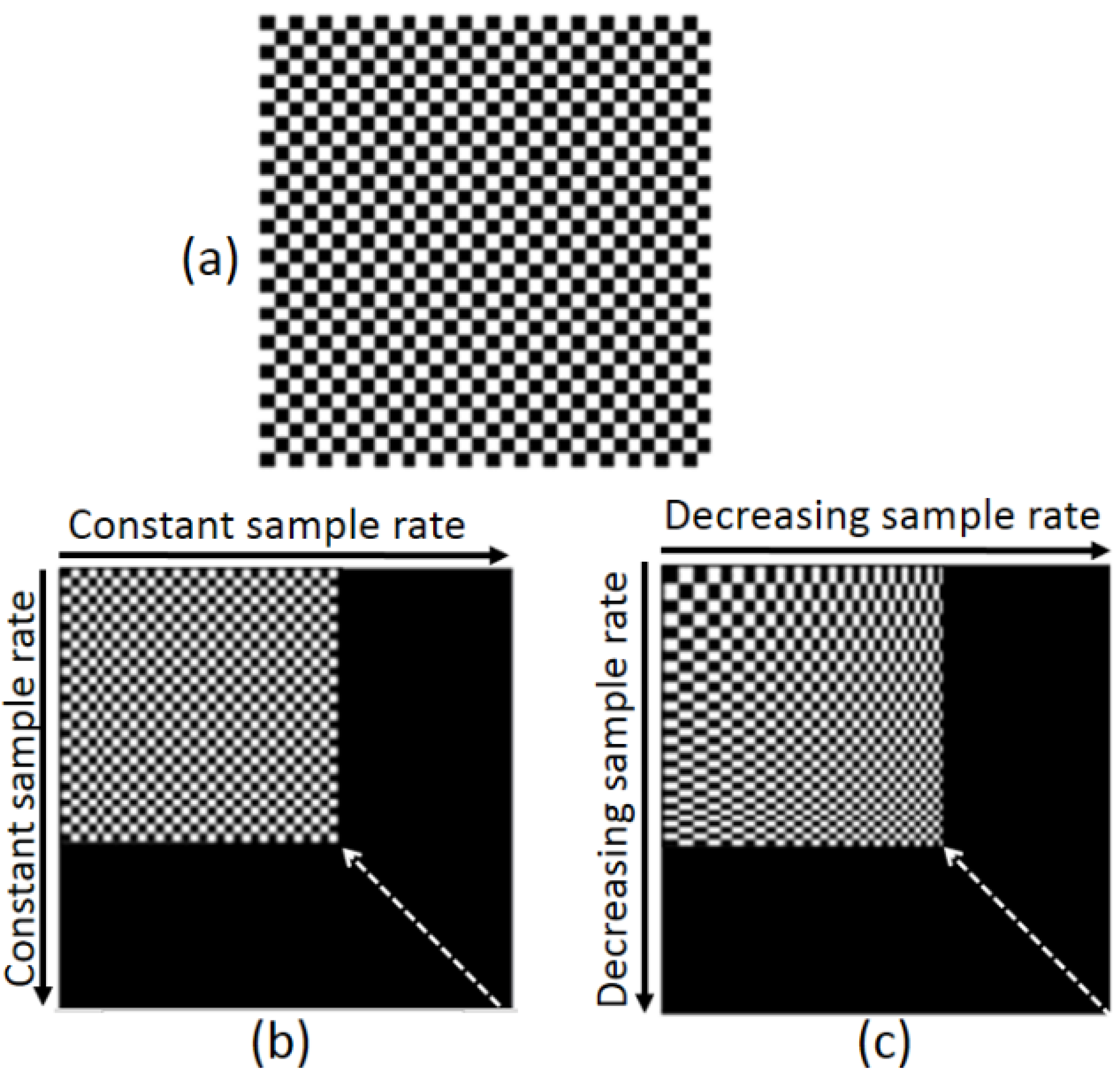
A visual comparison of nonelastic downsampling versus elastic downsampling is shown in Figure 5, where elastic and nonelastic methods are represented. In both cases, the number of samples is the same, but in the elastic method, the top-left corner is sampled with a higher sample rate (suppose that this corner has a higher PR value). Consequently, the top-left corner is more protected than the rest of the block.

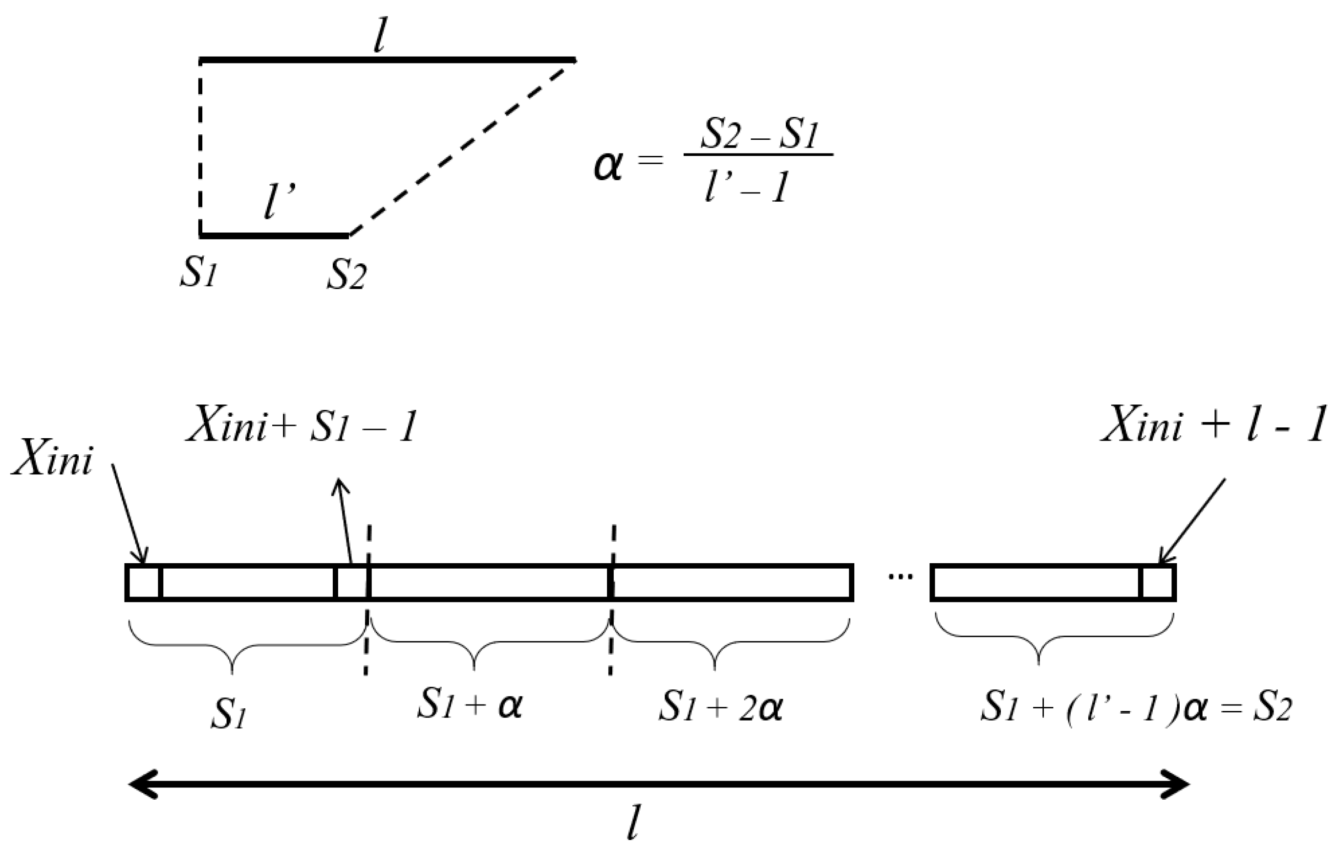
Given a vector of S values assigned to each corner, the equations to perform the Elastic Downsampling must consider an arithmetic series (Figure 6), which summation must match the entire edge of the block. In (Figure 6), $S1$ and $S2$ are the sample rates at block corners, and $\alpha$ is the sampling rate gradient.

Elastic downsampling is defined as a dimensionally independent mathematical operation. Due to that, this operation can be performed across dimensions indistinctly, like in any conventional (nonelastic) downsampling operation. For that reason, it is possible to first carry out a horizontal Elastic Downsampling and then a vertical elastic downsampling (or vice versa).

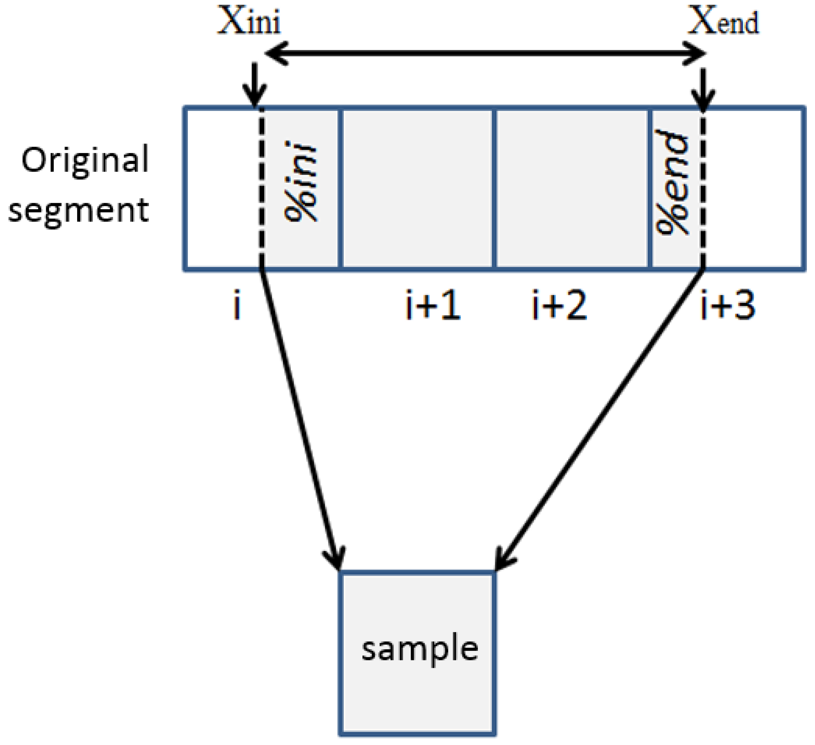
To compute the sample value, it is possible to use an average value of the pixels of the sample (in Figure 7, sample starts partially on $X_{ini}$ and finishes partially on $X_{end}$) or a single pixel selection (SPS). Empirical results show that the former produces better. As depicted in Figure 7, a sample may partially cover one or two pixels. This circumstance must be considered when computing sample values Equation (9). In Equation (9), $\%ini$ is the percentage of pixel i considered in the sample pixel, and $\%end$ is the percentage of pixel $i+3$ considered in the sample pixel.

$$\begin{array}{c}\hfill sample\text{\_}value={\displaystyle \frac{\%ini·value\left[i\right]+value[i+1]+\dots +\%end·value[i+3]}{X_{end}-X_{ini}}}\end{array}$$

(9)

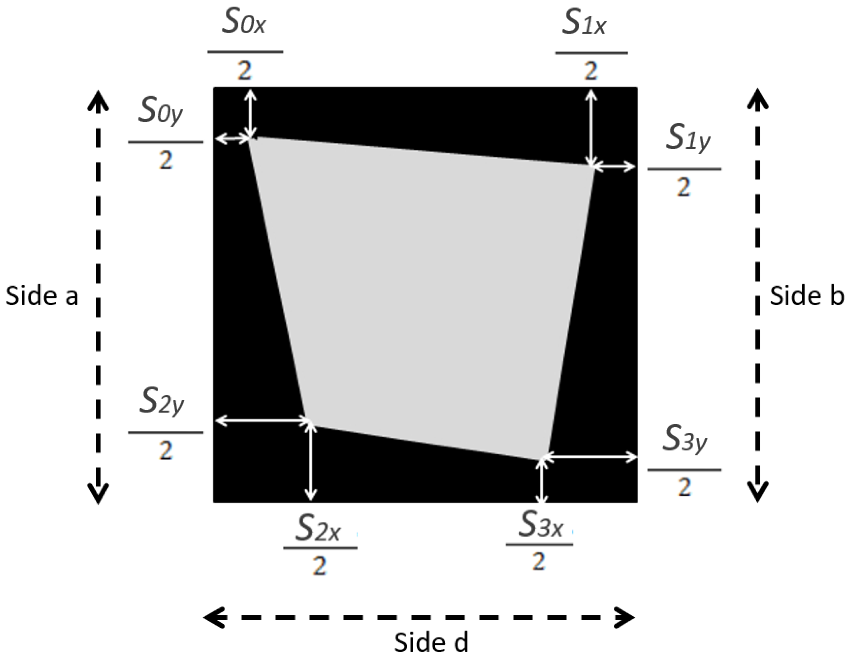
The final shape of a downsampled block must be a rectangle, so it can be processed by any filter or image compression algorithm. Equations (10) and (11) describe the required rectangular condition that has to be satisfied by the sample rates $S_{ij}$. The index i refers to the rectangle corner (0 is top-left, 1 is top-right, 2 is bottom-left and 3 is bottom-right). Index j refers to the space dimension (x refers to the horizontal dimension and y refers to the vertical dimension).

$$\begin{array}{ccc}\hfill S_{0x}+S_{1x}& =& S_{2x}+S_{3x}\hfill \end{array}$$

(10)

$$\begin{array}{ccc}\hfill S_{0y}+S_{1y}& =& S_{1y}+S_{3y}\hfill \end{array}$$

(11)

As a consequence, this rectangular condition implies that the sample rate values based on PR values have to be adjusted before the elastic downsampling process is carried out.

Algorithm 2 illustrates the procedure.

Algorithm 2 Elastic downsampling.

1: # $S_x\left[0\right],S_x\left[2\right]$ #initial and final rates for top edge a  2: # $S_x\left[1\right],S_x\left[3\right]$ #initial and final rates for bottom edge b  3: $S_{xa}=S_x\left[0\right]$ #initial rate for top edge  4: $S_{xb}=S_x\left[1\right]$ #initial rate for bottom edge  5: $gra{d}_{S_{xa}}=(S_x\left[2\right]-S_x\left[0\right])/l$  6: $gra{d}_{S_{xb}}=(S_x\left[3\right]-S_x\left[1\right])/l$  7: for$y=\{bloc{k}_{y_{start}}\dots bloc{k}_{y_{end}}\}$do  8:     $gra{d}_S=(S_{xb}-S_{xa})/(l^{\prime }-1)$  9:     for $x^{\prime }=\{bloc{k}_{x_{ini}}\dots bloc{k}_{x_{ini}}+l^{\prime }\}$ do 10:         # Addition of initial % 11:         $Percent=x_{ini}-\lfloor x_{ini}\rfloor$ 12:         $color+=image[x,y]\times Percent$ 13:         for $x=\{x_{ini}+1\dots \lfloor x_{ini}+S_x\rfloor \}$ do 14:            $color+=image[x,y]$ 15:         end for 16:         # Addition of last % 17:         $Percent=x_{ini}+Sx-\lceil x_{ini}+S_x\rceil$ 18:         $color+=image[x,y]\times Percent$ 19:         $color=color/S_x$ 20:         $imag{e}_{down}[x^{\prime },y]=color$ 21:         $S_x=S_x+gra{d}_S$ 22:         $x_{ini}=x_{ini}+S_x$ 23:     end for 24:     $S_{xa}=S_{xa}+{\alpha }_{S_{xa}}$ 25:     $S_{xb}=S_{xa}+{\alpha }_{S_{xb}}$ 26: end for

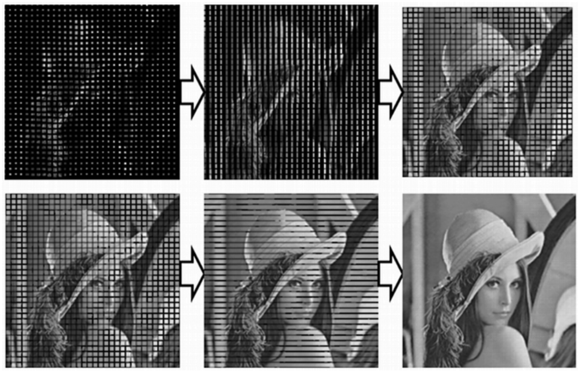
5. Proposed Elastic Interpolation Method

This section describes elastic interpolation: the inverse process to elastic downsampling. This is the method used to scale the blocks back to their original size. Like the downsampling, the interpolation is a separable operation and it can be executed in each dimension sequentially (Figure 8).

To carry out the elastic interpolation, the involved gradients of sample rates are required. They are used to reconstruct the correct number of pixels per sample for each interpolated scanline.

The horizontal sample rate at the vertical left side (notated as side a) of each block evolves from $S_{0x}$ to $S_{2x}$. This sample rate ($S_a$) is the initial sample rate for each scanline from the side a to side b (vertical right side of the block). At side b, the horizontal sample rate evolves from $S_{1x}$ to $S_{3x}$. Therefore, each scanline evolves from $S_{ax}$ to $S_{bx}$ across the length c, (side c is the horizontal top side of the block and is equals to the horizontal bottom side d, because of the rectangular condition). Equations for horizontal interpolation are the following:

$$\begin{array}{ccc}\hfill gra{d}_a& =& (S_{1x}-S_{0x})/l_a\hfill \end{array}$$

(12)

$$\begin{array}{ccc}\hfill gra{d}_b& =& (S_{3x}-S_{2x})/l_b\hfill \end{array}$$

(13)

$$\begin{array}{ccc}\hfill S_a& =& gra{d}_a·y\hfill \end{array}$$

(14)

$$\begin{array}{ccc}\hfill S_b& =& gra{d}_b·y\hfill \end{array}$$

(15)

$$\begin{array}{ccc}\hfill gra{d}_{scanline}& =& (S_b-S_a)/l_c\hfill \end{array}$$

(16)

where ${grad}_a$ is the sampling rate gradient at side a, $S_a$ is the sampling rate of side a at position y, ${grad}_b$ is the sampling rate gradient at side b, $S_b$ is the sampling rate of side b at position y, and ${grad}_{scanline}$ is the sampling rate gradient at horizontal scanline located at position y. The lengths of the different sides are $l_a$, $l_b$ and $l_c$.

Despite having a higher complexity, bilinear interpolation provides a higher quality than nearest neighbor interpolation in terms of PSNR. The first sample represents a group of pixels and is located in the middle of them. Therefore, the values before the location of the sample must be interpolated considering the previous block.

Additionally, due to the values of $S_{0x}$ and $S_{1x}$ are not equal, and $S_{0y}$ and $S_{1y}$ may be also different, the resulting interpolated block will probably not be a square but a trapezoid (Figure 9).

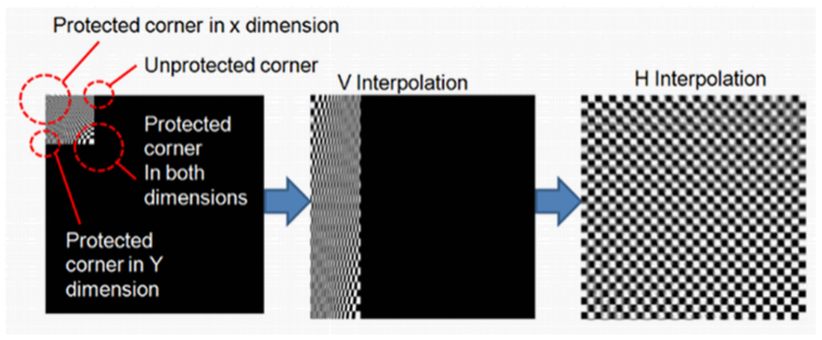
Elastic bilinear interpolation is composed of two stages: first, an interpolation of individual blocks, and second, the seams interpolation, which must be performed after the block interpolation has been processed for all blocks. The seam interpolation process is shown in Figure 10 and it is carried out first vertically and then horizontally.

6. Experimental Results

The proposed elastic downsampling technique has been validated against the Kodak image dataset [20] (24 natural images of size $768\times 512$ in PNG format released by the Kodak Corporation for unrestricted research usage) and the USC Miscelanea gallery [19] (44 images of different features including famous “lena”, “baboon”, etc.) The experimental results show a clear benefit at any sampling ratio.

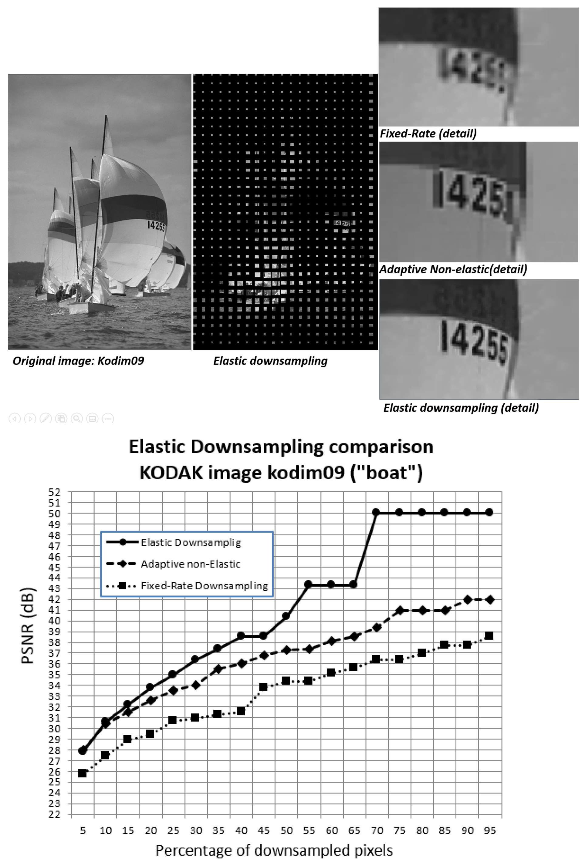
Figure 11 presents the comparison of the resulting PSNR (after the interpolation process) between a fixed-rate downsampling, an adaptive nonelastic downsampling, and the proposed elastic downsampling schemes. In all cases the interpolation type is bilinear. The sampling rates per block in adaptive nonelastic downsampling were assigned considering the PR metric. All curves tend to the same values when the percentage of samples is very low. The KODAK gallery improvement against fixed-rate is between 1.48 dB at the lowest sampling rates (5% samples) and up to 15.0 dB for the highest gains (95% of samples). The average advantage is 6.8 dB. The USC gallery average benefit is 2.94 dB and the highest is 14.5 dB. The advantage against adaptive nonelastic is lower, from 0.5 dB to 1dB for both galleries. In this case the benefit is more subjective (less artifacts) than objective (metrics).

In addition to the PSNR advantages, all the resulting images do not present blocking effects nor artifacts at any compression factor, thanks to the sampling rate continuity between adjacent blocks.

Additionally, Figure 11 also shows how elastic downsampling preserves quality at high sample rates (even better than adaptive nonelastic downsampling. Damage does not occur in relevant parts of the image, but only in nonrelevant areas, thus producing a higher PSNR. For comparison, fixed pixel-rate downsampling damages relevant and nonrelevant areas in the same proportion, thus producing a drastically lower PSNR. Both curves tend to the same values when the percentage of samples is very low. The greatest advantage (15.0 dB) is obtained with 95% of samples and the smallest (1.48 dB) with 5% of samples. On average the advantage is 6.8 dB.

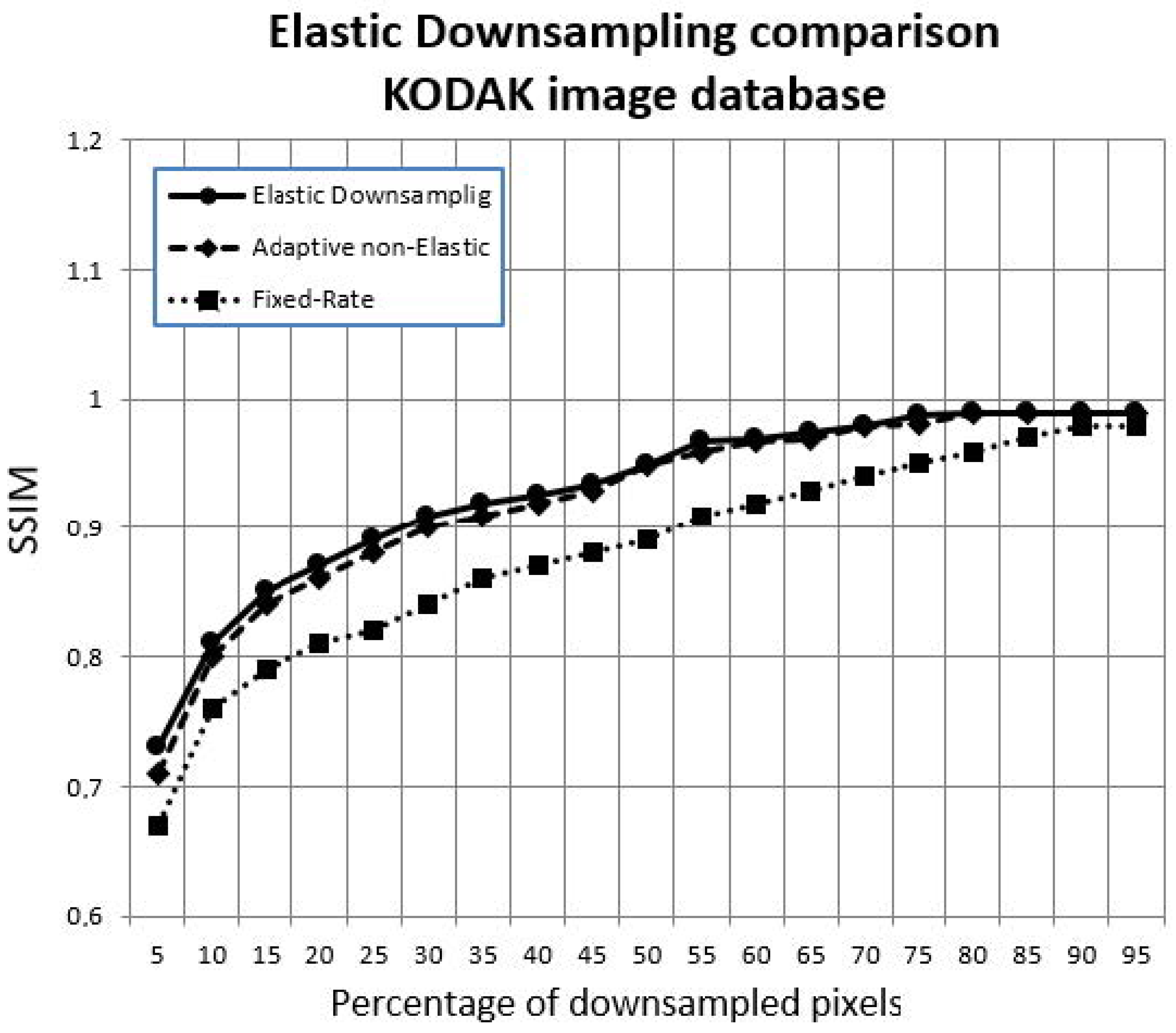
Regarding the SSIM metric, a comparison between adaptive nonelastic and elastic downsampling (Figure 12) reveals very similar curves, slightly better with elastic downsampling, but not as significant as with the PSNR metric.

A visual comparison between conventional (fixed-rate), adaptive nonelastic, and elastic downsampling is shown in Figure 13. It clearly shows that the boat and sail details, especially the numbers, are better protected with the elastic downsampling.

The same visual comparison for the image “motorcycles” is shown at Figure 14. In this case the advantage is not so extreme but is clear and the helmet details are better protected with elastic downsampling. For both images (boat and motorcycles), there are no blocking effects nor artifacts present, thanks to the smooth sample rate evolution, which is a benefit of elastic downsampling.

7. Discussion

This section presents the benefits and limitations of the proposed elastic downsampling method and describes its application for real-time video through two implementations.

7.1. Benefits and Limitations

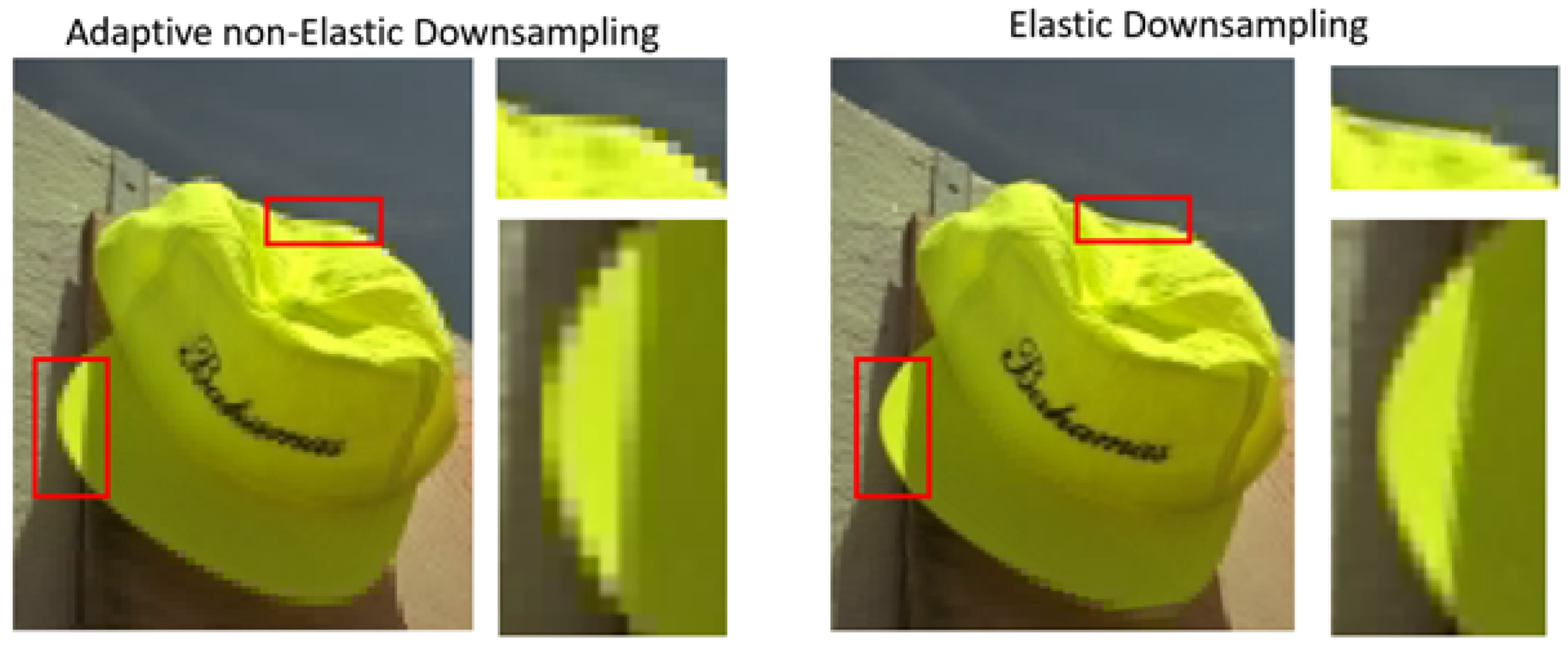
Considering PSNR metrics, elastic downsampling shows better (but similar) results when compared to adaptive nonelastic downsampling. However, when compared with fixed sample rate sampling the improvement is considerable. In our experiments, performed over two image sets, the average difference with nonelastic is around 1 dB, but it is important to note that the proposed method also offers a subjective improvement in quality, thanks to the reduction of potential artifacts at blocks’ boundaries (Figure 15).

Block boundaries may show artifacts at nonelastic adaptive downsampling and this drawback is overcome by elastic downsampling. However, depending on the image structure and location of every object with respect to block boundaries, the obtained benefit when comparing to nonelastic adaptive downsampling may range from dramatic to almost indistinguishable. For instance, a very homogeneous image, such as clouds, fur, or noise does not benefit from elastic downsampling, since perceptual relevance is constant across the image. Therefore, all corners get a similar sample rate and the result is comparable to downsampling using fixed sample rate. The benefit is more apparent when high relevance areas are combined with low relevance areas in the same image.

Finally, it must be highlighted that the PR has been computed on luminance, and the resulting metric has been applied to both luminance and chrominance components. Although not very common, an image that shows more contrast in chrominance than luminance will see reduced benefits from our proposed methods. Future improvements will focus on chrominance PR metrics.

7.2. Application for Real-Time Video: LHE Codec

This downsampling mechanism is suitable for encoding images and videos that do not need strict 8 × 8 or 16 × 16 resulting blocks, as is the case for a DCT-based encoding solution. Blocks bigger than 8 × 8 are more suitable to benefit from elastic downsampling, since there are potentially bigger Perceptual Relevance differences between corners. As a case study for this work we chose the Logarithmical Hopping Encoding [21] (LHE) codec: a fast spatial-based compressor able to process blocks/rectangles of any size. This codec was designed for real-time video applications and its main phases are shown in Figure 16. The downsampling process comprises two of these stages: horizontal and vertical.

An experimental implementation of elastic downsampling was developed using CUDA 8 and run on an Nvidia Geforce GTX-1070 GPU (NVIDIA, Santa Clara, CA, USA). This implementation involves the PR computation and, as already stated, separate horizontal and vertical downsampling steps. These three phases put together take 35% of the total computation time for the LHE compression process (1 ms for a vertical resolution of 720 pixels with a 16:9 aspect ratio).

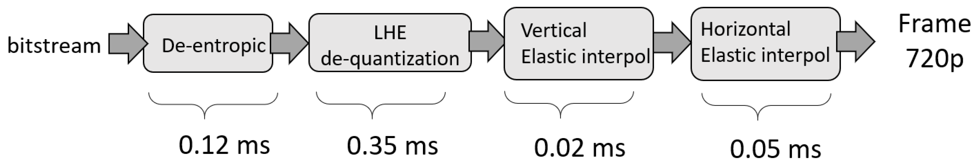
At the decoder side, the interpolation process takes fewer computing resources: around 10% of the total decompression time (Figure 17). This technique does not show any blocking effect at any compression level and takes around 0.55 ms tested on an Nvidia Geforce GTX-1070 GPU.

Another experimental implementation using a low-cost device (Raspberry Pi3) was also developed. This solution benefits from the four cores available in the hardware, allowing for a parallel execution of the elastic downsampling. This implementation was created following the same phases as Figure 16 with certain limitations such as the resolution (640 × 480) and the type of downsampling (single pixel selection, SPS, instead of the average method). The PR computation and downsampling phases of this implementation also took roughly 35% of the total compression time (11 ms). Since the device was intended for video transmission, the decoding phases (Figure 17) were not implemented in the Raspberry Pi.

8. Conclusions

This paper describes an adaptive downsampling technique based on a novel Perceptual Relevance metric and a new elastic downsampling method. Experimental results were presented to provide a comparison between nonelastic downsampling schemes and elastic downsampling.

Based on the results, elastic downsampling has been proven to provide:

• A reduction of spatial image information; a feature desirable for picture processing, storage, and transmission.
• Improvements in the adaptive downsampling stage of spatial compressors such as the LHE (Logarithmical Hopping Encoding) codec [21].

Additionally, the main advantages of the elastic downsampling algorithm are:

• High protection of image quality, improving from 1.5 dB to 15 dB compared with nonelastic downsampling methods (average 6.8 dB).
• No blocking effects, thanks to the sampling rate continuity between adjacent blocks.
• A linear and mathematically separable procedure, which allows for an easy implementation.

Finally, the proposed method has been successfully tested on a real-time video codec (LHE) in two different platforms: a GPU-based system and a low-cost device.

The results of this paper point to several interesting directions for future developments:

• PR analysis for the chrominance signal, improving the quality of color, particularly on images with heavy chrominant contrast.
• Comparison of elastic downsampling with upscaling methods, which share the same goal; to obtain a better quality image using less information.
• Improve the elastic interpolation algorithm: Where a downsampled pixel frontier does not match with an upsampled pixel frontier, an accurate mix of downsampled pixels could increase the fidelity of the upsampled pixel, improving final quality.
• Test on more image galleries of different nature, such as cartoons or computer graphics.