Article

Optimising Hardware Accelerated Neural Networks with Quantisation and a Knowledge Distillation Evolutionary Algorithm

1
Mathematical and Computer Sciences, Heriot-Watt University, Edinburgh, EH14 4AS, UK
2
Inria Rennes-Bretagne Altlantique Research Centre, 35042 Rennes, France
3
Lab-STICC, École Nationale Supérieure de Techniques Avancées, 29200 Brest, France
*
Author to whom correspondence should be addressed.
Electronics 2021, 10(4), 396; https://doi.org/10.3390/electronics10040396
Submission received: 28 December 2020 / Revised: 27 January 2021 / Accepted: 1 February 2021 / Published: 5 February 2021
(This article belongs to the Special Issue Recent Advances in Embedded Computing, Intelligence and Applications)

Abstract

:
This paper compares the latency, accuracy, training time and hardware costs of neural networks compressed with our new multi-objective evolutionary algorithm called NEMOKD, and with quantisation. We evaluate NEMOKD on Intel’s Movidius Myriad X VPU processor, and quantisation on Xilinx’s programmable Z7020 FPGA hardware. Evolving models with NEMOKD increases inference accuracy by up to 82% at the cost of 38% increased latency, with throughput performance of 100–590 image frames-per-second (FPS). Quantisation identifies a sweet spot of 3 bit precision in the trade-off between latency, hardware requirements, training time and accuracy. Parallelising FPGA implementations of 2 and 3 bit quantised neural networks increases throughput from 6 k FPS to 373 k FPS, a 62 × speedup.

1. Introduction

Neural networks have proved successful for many domains including image recognition, autonomous systems and language processing. State-of-the-art models have an enormous number of parameters, making them highly computationally and memory intensive. For example, AlexNet [1] is a Convolutional Neural Network (CNN) consisting of 60 million parameters and 650 k neurons with an architecture comprising five convolutional layers, multiple max-pooling layers, three fully-connected layers and a final softmax layer. GPUs are often used to train and use neural networks because they can deliver the highest peak arithmetic performance for 32 bit floating point neural network inference compared with CPUs and FPGAs. At the time when the AlexNet model was proposed (2012), the network was too large to fit on a single GPU. This problem was overcome by distributing the model across two GPUs for training. The use of 200+ Watt GPUs for such purposes over days and weeks is prohibitively expensive [2].
In recent years, a new class of hardware has emerged to significantly improve performance-per-Watt for deep learning. Accelerator devices such as the Intel Movidius Myriad X VPU [3] and the Coral/Google Edge TPU [4] accommodate deep learning workloads because they provide a trade off between compute performance and power consumption. The extreme on the hardware spectrum is programmable hardware like FPGAs, which provide extremely high throughput performance of fixed-point deep learning inference [5]. This is essential for real-time domains with low latency throughput requirements, e.g., remote computer vision and automated stack market trading.
It is widely accepted that neural network models exhibit a high level of redundancy. Most parameters contribute little or nothing to the final output [6], and the precision of arithmetic calculations are unnecessarily precise [7]. Removing redundant bloat offers the opportunity of mapping sophisticated models to energy efficient devices. Methods for compressing neural networks include precision reduction, removing redundant parameters or structure, and transferring knowledge from large models to smaller models [8].
The aim of compression is usually to reduce the hardware footprint of a model to increase its inference throughput (decreasing its inference latency), without overtly affecting inference accuracy.
Compressing neural network can:
  • Speed up inference time: The size of neural network models are limited by memory capacity and bandwidth. Training and inference computations switch from compute-bound to memory-bound workloads as model sizes increase. This memory capacity bottleneck limits the practical use of very large models [9].
  • Improve energy efficiency: It costs orders-of-magnitude more energy to access off-chip DDR memory compared to on-chip memory e.g., SRAM, BRAM and cache memory. Fitting weights into on-chip memories reduces frequency of energy inefficient off-chip memory accesses. Quantised fixed-point representations can significantly reduce energy costs [10], e.g., less than 5 Watts on FPGAs [11].
  • Reduce verification costs: Recent SMT-based verification approaches aim to prove a neural network’s robustness against adversarial attacks e.g., [12,13]. SMT solvers generally do not support non-linear arithmetic so activation functions must be linearised. This approximates a model for the purpose verification, rendering verification results unreliable. Quantising activation functions can increase reliability of verifying neural networks robust [14], because it is the same model being verified and deployed. Moreover quantised models can be as robust against adversarial attack as their full precision version, possibly because quantisation acts as a filter of subtle adversarial noise [15].
Neural network models vary hugely in their sizes, i.e., from 60 thousand parameters up to 900 million parameters. Figure 1 shows how compression such as quantisation and knowledge distillation can put relatively large models within reach of high throughput hardware accelerators [16,17,18,19,20].
This paper evaluates the accuracy, throughput, training time and resource costs of two compression approaches applied to different sized models: (1) an evolutionary algorithm that modifies the structure of 16 bit precision neural networks targeting the Intel Movidius Myriad X VPU, and (2) 1–8 bit precision quantisation of fixed neural networks targeting the Xilinx Z7020 FPGA.

Contributions

This paper makes the following contributions:
  • A new framework called NEMOKD for hardware aware evolution of knowledge-distilled student models (Section 3).
  • An evaluation of neural network quantisation by measuring inference accuracy, throughput, hardware requirements and training time, targeting programmable FPGA hardware (Section 4.2).
  • An evaluation of NEMOKD showing its ability to minimise both latency and accuracy loss on Intel’s fixed Movidius Myriad X VPU architecture (Section 4.3).
  • A comparison of NEMOKD and quantisation performance on these architectures (Section 4.4).

2. Quantisation Methodology

2.1. Quantisation for FPGAs

Floating point precision permits individual neural network parameters a range of exponent values. Higher precision values (larger exponents) can induce more computational overhead, leading to higher power consumption and longer compute times. Fixed-point quantised models use (usually smaller) fixed exponent values for all network parameters. This imposed restriction brings a range of benefits such as faster and more power efficient mathematical operations but can also potentially impact a model’s accuracy [21].
  • Quantisation [22] shiftsvalues from 32 bit floating point continuous values to reduced bit discrete values. In a neural network, weights between neurons and activiation functions can be quantised.
  • Binarisation [23] is a special case of quantisation that represents weights and/or activation function outputs with a single bit. These methods replace arithmetic operation with bit-wise operations, reducing the energy consumption and memory requirements.
Quantised neural networks can signifiantly outperform binarised neural networks and can compete with the accuracy of full precision models [22].

2.2. FINN Framework

Section 4.2 evaluates very low precision neural networks, quantising precision from 32 bits to 1–8 bits to fit within the resource constraints of FPGAs. Xilinx’s FINN quantisation framework and FPGA backend is used in these experiments. FINN initially supported binarised neural networks [7], then was extended for quantised networks [24] and Long-Short Term Memory Neural Networks (LSTM) [25]. Our experiments in Section 4.2 use FINN functionality from [24].
FINN employs quantisation aware training at the Python level, before generating synthesisable C++ for hardware. The weights and activation functions during training in Python operate on floating point values but Python functions simulate quantisation to limit weights and activation function outputs to discrete values permitted by the chosen quantisation configuration. When generating hardware, the arithmetic precision of weights and activation functions in the C++ match the quantised bit widths simulated during training.

2.3. Weight Quantisation for Training

FINN discretises the range of full precision values by rounding to a close neighbour to fixed point quantised values for weights. The min and max values for the quantisation range are related to the quantisation precision n, they are defined as:
m a x = 2 1 2 n 2 m i n = 2 + 1 2 n 2
The quantisation formula for x [ m i n ; m a x ] is shown in Equation (1).
Q u a n t i s e W e i g h t s ( x ) = 2 n x + 2 n 1 1 2 n 2 2 + 1 2 n 2
Table 1 shows examples of quantised values with m i n = 2 and m a x = 2 with 2 n 1 values in this interval. The values are all strictly positive but the quantisation range is symmetric. The step between each quantised value is 1 2 n 2 . When n increases, the number of quantised values increase and we can obtain values close to the upper and lower bound of the interval.

2.4. Activation Function Quantisation for Training

The quantisation of activation functions works similarly to weight quantisation. For the quantised hyperbolic tangent function t a n h ( x ) = e x e x e x + e x , the range of values in Table 1 is optimal because the function has two asymptotes towards −1 and 1, e.g., t a n h ( 2 ) = 0.964 . The saturation plateau of the activation function is almost attained. Figure 2 shows the shape of tanh for different quantisation precisions.

3. NEMOKD: Knowledge Distillation and Multi-Objective Optimisation of Neural Networks

This section presents our new NEMOKD framework. Its aim is to produce accurate neural networks small enough to fit onto hardware accelerators to achieve high throughput. Section 3.2 describes its knowledge distillation based training. Section 3.3 shows its multi-objective optimisation that evolves encoded neural network hyper-parameters to find optimal trade-offs between accuracy and throughput. Section 3.4 presents the NEMOKD methodology for hardware-aware optimisation, which measures inference latency on the intended target device to feed into the evaluation of evolved CNN architectures.

3.1. Evolutionary Algorithms

Evolutionary deep learning approaches [26] have been proposed as an alternative training approach to stochastic gradient descent. However, due to the enormity of the search space for state-of-the-art neural networks that comprise millions of parameters, evolutionary algorithms often fail to discover optimal solutions.
Recent neuro-evolution techniques retain stochastic gradient descent and back propagation for training, before using evolutionary algorithms to search for optimal architectural configurations. Device-aware Progressive Search for Pareto-Optimal Neural Architectures [27] is a method of neural architecture search that has been shown to simultaneously optimise device-related objectives such as inference time and device-agnostic objectives such as accuracy. This search algorithm uses progressive search and mutation operators to explore the trade-offs between these objectives. Applying this algorithm to problems on a range of different hardware devices from a NVIDIA Titan X GPU to a mobile phone with an ARM Cortex-A35, the authors of [27] were able to obtain higher accuracy and shorter inference times compared to the state-of- the-art CondenseNet [28].
Neural-Evolution with Multi-Objective Optimisation (NEMO) [29] is a neural network optimisation algorithm. It is a machine learning technique that uses multi-objective evolutionary algorithms to simultaneously optimise both accuracy and inference time of neural networks by evolving their architecture.

3.2. Knowledge Distillation

Neural networks often have a softmax output layer that produce probabilities of given inputs belonging to each class. The cross entropy loss function measures the similarity of the softmax output vector against a ground truth vector defined by the training set. Given ground truth label vector y , N classes in the vector, and a softmax prediction vector p , the cross entropy loss is:
H ( y , p ) = i N y i ln ( p i )
Knowledge distillation incorporates an additional hyper-parameter, temperature (T), into this softmax calculation. Softer probability distributions over classes are obtained by using higher temperatures [8]. Knowledge distillation employs a loss function that uses two weighted objective functions:
1.
Student loss: cross entropy of the student’s standard softmax output ( T = 1 ) with the ground truth vector.
2.
Distillation loss: cross entropy of the teacher’s high temperature ( T = τ ) output with the students high temperature output.
The loss function for knowledge distillation (from [30]) is:
L ( x ; W ) = α H ( y , σ ( z s ; T = 1 ) ) S t u d e n t L o s s + β H ( σ ( z t ; T = τ ) , σ ( z s ; T = τ ) ) D i s t i l l a t i o n L o s s
where x is an input, W are the parameters of the student network, y the ground truth vector and σ ( z ; T = τ ) is the softmax function applied to logit vector z and temperature T = τ . The student and teacher logit vectors are s and t, and hyper-parameters α and β are arbitrary constants.
In the NEMOKD methodology (Section 3.4), student models in the initial CNN architecture population are partially trained using knowledge distillation.

3.3. Multi-Objective Optimisation

Multi-Objective Optimisation solves optimisation problems with at least two conflicting objectives. For a solution space A that contains all permissible neural networks configurations, the two objectives of NEMOKD are (1) minimise inference latency (latency) and (2) minimising accuracy loss (error):
m i n a A ( l a t e n c y ( a ) , e r r o r ( a ) )
NEMOKD generates this solution space A by encoding and evolving hyper-parameters of student models (Section 3.3.1) then evolving these to optimise for Equation (4) (Section 3.3.2).

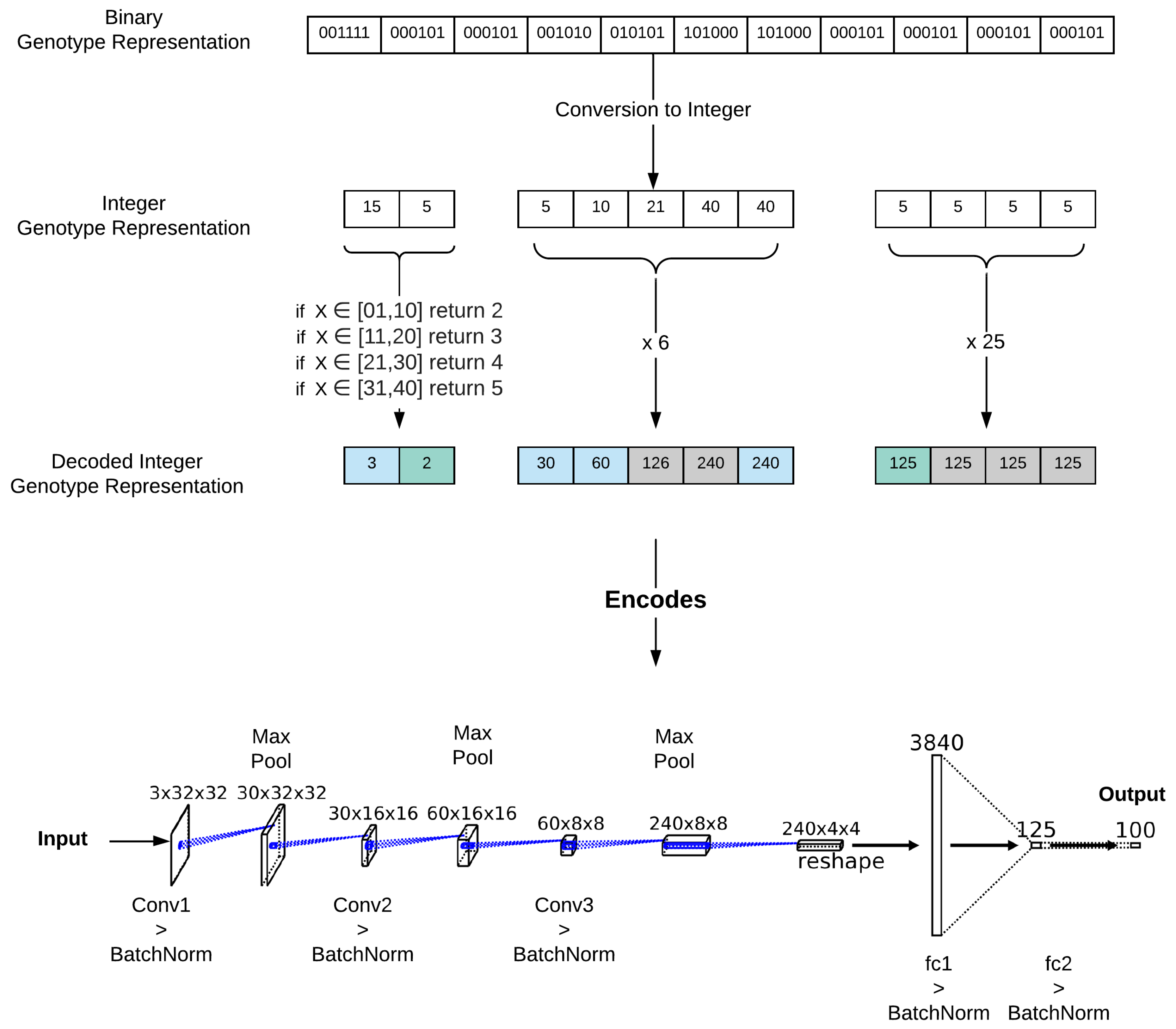
3.3.1. Encoding Student Models for Evolution

The evaluation of NEMOKD in Section 4.3 uses two baseline student architectures: FlexStudent and Resnet8x4. We encode certain features of these model into genotypes to evolve their hyper-parameters.
We encode the FlexStudent model with 11 genes. Genes 1 and 2 determine the number of convolutional and fully connected layers respectively. Genes 3–7 determine the number of output channels in convolutional layers. Genes 8–11 encode the number of fully connected layers. Figure 3 shows how NEMOKD decodes the genotype representation of the baseline FlexStudent model into a CNN architecture.
For the Resnet8x4 student we encode hyper-parameters to evolve the number of layers in the output channels from convolutional layers. The number of layers are fixed.

3.3.2. Multi-Objective Evolution

We employ the Non-Dominated Sorting Genetic Algorithm version II (NSGAII) [31] to facilitate evolutionary multi-objective optimisation, starting from the baseline architecture trained with knowledge distillation. Model mutations with NSGAII are both fine and coarse grained. Mutation in our NEMOKD framework modifies four hyper-parameters:
1.
The number of convolutional layers.
2.
The number of Fully Connect layers.
3.
The number of output channels.
4.
The number of Fully-Connected neurons.
NEMOKD uses NSGAII to generate a set of CNN architecture solutions from one population member. Student models (either FlexStudent or Resnet8x4) are first encoded into a genotype sequence (Figure 3). The evolutionary process then happens in two steps: (1) crossover generates a new solution by combining genotypes of two parents; (2) ranking and selection chooses the fittest members of the population, based on the best trade-off between accuracy and latency when evaluated on the VPU. For every solution, mutation alters one or more genes at random.
For the two objectives of minimising latency ( f 1 ) and error ( f 2 ), a solution a dominates solution b if it outperforms for one of these objectives and is not worse in the other:
i [ 1 , 2 ] , j [ 1 , 2 ] : f i ( a ) f i ( b ) a n d f j ( a ) < f j ( b )
NEMOKD uses NSGAII to search for Pareto optimal solutions. A CNN architecture solution a is Pareto optimal if it is not dominated by any other solution in a solution space A:
b A , i [ 1 , 2 ] , j [ 1 , 2 ] : f i ( a ) f i ( b ) a n d   f j ( a ) < f j ( b )   a n d   a     b
The final output from NEMOKD is a population of evolved models, which includes those in the Pareto optimal set.

3.4. NEMOKD Methodology

The NEMOKD methodology combines knowledge distillation and the multi-objective evolutionary algorithm above. The methodology comprises two phases:
  • Phase 1: Knowledge Distillation: A baseline model is trainedwith knowledge distillation to provide a comparison for NEMOKD performance. NEMOKD uses that baseline architecture as a starting point to generate variants using evolutionary multi-objective optimisation.
  • Phase 2: Model Evolution: Each generation produces 10–20 variations of the baseline model, each then trained using knowledge distillation. The two objectives, minimising latency and minimising error, are measured for each model on the VPU device. The Pareto optimal models are retained to form part of the next generation. The other models are discarded. This process repeats for a specified number of generations. In our NEMOKD evaluation (Section 4.3), generations range from 14 to 27.
The NEMOKD methodology is shown in Figure 4. A population N is initialised. Each member of this population is a genotype that represents a CNN student architecture in the solution space (Section 3.3.1). To increase the chance of finding comparable or better solutions in a small number of generations, random perturbations are then applied to half the population to encourage more diverse solutions.
First, each genotype is decoded to construct a CNN model. These are then partially trained with knowledge distillation and are then converted to the ONNX format and finally a half-precision Intermediate Representation for VPU deployment. The fitness of each individual genotype is then assessed on the VPU device based on accuracy and latency performance. Genotype evaluation results are passed to NSGAII for evolution of student model hyper-parameters (Section 3.3.2).
NSGAII selects genotypes based on their fitness values to add new members. Crossover and mutation are applied to this member set, to add to the overall population. This evolve/ decode/select process repeats until a specified number of NEMOKD generations. The algorithm outputs the final population including the Pareto optimal set (Equation (6)). This set of solutions provides optimal trade-offs between the two objectives in the objective space.

3.5. NEMOKD versus NEMO

Our NEMOKD methodology extends NEMO [29] in three ways:
  • Knowledge distillation replaces standard training in the learning phase of the evaluation procedure.
  • To conserve time and computational resources in the learning phase, partial training is provided with only 30 epochs (in phase 1) as opposed to fully training each member of initial population.
  • Latency and accuracy is measured on the VPU device to asses the fitness of population members. This evaluation data is fed into the evolutionary NSGAII algorithm.
Accuracy after 30 epochs is indicative of performance should full training later be performed. Therefore to save time and energy costs of fully training all evolving student variants, a developer might select a fully evolved partially trained model that meets latency requirements, then subject it to more training with 200+ epochs.
We say NEMOKD’s evolutionary optimisation is hardware-aware, because fitness is measured on the processor architecture (Intel’s Movidius VPU) intended for deploying the model. This is based on the idea that a model’s latency performance depends on the processor architecture used, and that optimising a model for one architecture may be ineffective if deploying to another [27].

4. Evaluation

4.1. Hardware Platforms

This section evaluates quantisation for programmable hardware, and our NEMOKD evolutionary algorithm for the fixed VPU architecture. The dataset and neural network model for the experiments are shown in Table 2.
For the programmable hardware experiments we target the mid-range Xilinx Zynq Z7020 140 mm × 87 mm FPGA on the Xilinx PYNQ-Z2 development board which uses ≈13.8 W energy. This FPGA has 53 k Lookup Tables (LUT), 106 k Flip Flops (FF) and 560 KB of Block RAM (BRAM) memory. Of the 64 quantised neural networks in Section 4.2, only four fit on this FPGA. This validates the need for aggressive compression approaches such as quantisation, on small to medium sized FPGA devices.
For the fixed hardware experiments we use a USB-based Intel Neural Compute Stick 2 (NCS2) accelerator using a 72.5 mm × 27 mm Intel Movidius Myriad X Visual Processing Unit (VPU) which uses ≈1.5 W energy. The NCS2 comprises dedicated accelerators with the 16 programmable 128-bit VLIW Vector Processors optimised for processing highly parallel workloads. The device can compute up to 1 Tera Operation Per Second (TOPS). The centralised 2.5 MB of on chip memory facilitated by the intelligent memory fabric enables memory access latencies of 400 GB/s and reduces the requirements for more costly off-chip data transfer. The NCS2 device has 512 MB of LPDDR4 memory [3].

4.2. Quantisation Results

This section investigates the design space granted by FINN’s ability to independently quantise weights and activation functions of a Multilayer Perceptron (MLP) network with three Fully-Connected (FC) layers. We created 64 quantised models from a baseline model by independently and exhaustively varying the bit-widths of weights and activation functions from 1 to 8. For 64 neural network quantisation configurations, the evaluation in this section measured:
(1)
Absolute accuracy and hardware resource costs of the 64quantised neural networks (Section 4.2.1).
(2)
Relative performance comparison of accuracy and hardware resource costs, compared with the other 63 quantised models (Section 4.2.2).
The training was done using 50,000 images from the MNIST dataset. A validation dataset of 10,000 images was then used to minimise overfitting. Accuracy was measured using a testing dataset, to test how well the model generalised to new data. FINN’s backend converted the model to a binary weight file and a synthesisable C++ implementation for hardware.

4.2.1. Absolute Performance

Absolute Accuracy Performance

Each of the 64 neural networks was labelled with a quantised weight W-X and quantised activation function A-Y with X , Y [ 1 ; 8 ] . Accuracy is measured after 10, 20, 30, 50 and 100 epochs.
Figure 5 plots the inference error rate for each of the 64 quantised neural networks after training with 10, 20, 30, 50 and 100 epochs. Using 1–3 bits weights had a noticeable effect on accuracy, i.e., between 3.9–4.7% dropping down to below 3.7% using 4 bits or more. Training further with 40–100 epochs shifted the noticeable accuracy boundary to just 1 bit weight, meaning that with enough training, 2 bit weights achieved almost the same inference accuracy as 3–8 bit weights. The quantisation of activation functions had a steady impact on accuracy, i.e., higher precision activation functions result in better accuracy, however, this was not as dramatic as the impact that quantised weight precision has on accuracy. With increased training time, the accuracy performance flattened, where absolute difference in accuracy between the best and worst quantisation configuration greatly diminished. Additionally, we observed a major gap between 1 and 2 bit weights versus 3–8 bit weights, especially for 10 and 20 epochs. Training beyond 40 epochs allowed weights to be quantised from 3 to 2 bits without noticeable accuracy loss.

Absolute Resource Utilisation Performance

Figure 6 shows the trade-off between quantised precision and hardware resource use. The X axis is the number of bits for weights, the Y axis is the number of bits for the activation functions. The colour in the heat maps represents the relative measurement of the respective performance metric compared to the other 63 models.
Figure 6a shows that both weight precision and activation function precision contributed evenly to LUTs costs. Figure 6b shows that the precision of activation functions determined FF costs. While FFs and LUTs could store small amounts of data, BRAMs had greater storage capacity and were used by hardware synthesis tools for larger data structures such as arrays. Figure 6c shows that BRAM consumption was determined exclusively by weight precision.

4.2.2. Relative Performance

Table 3 gives the best and worst relative performance numbers for the 64 quantised neural networks. The three radar plots in Figure 7 represents different quantised neural network configurations, comparing accuracy and resource use (LUTs, FFs and BRAMs) performance relative to the best and values in Table 3. Each metric defines one branch in a radar chart. The three precision variations in Figure 7 are:
  • Weight oriented distribution (Figure 7a) increased the weight precision and kept the activation function constant at 4 bits, i.e., W1–A4, W3–A4, W6–A4 and W8–A4.
  • Activation oriented distribution (Figure 7b) increased the activation function precision and kept the weight precision constant at 4 bits, i.e., W4–A1, W4–A3, W4–A6 and W4–A8.
  • Linear distribution (Figure 7c) increased both the weight and activation function precision across the diagonal from the heat maps in Figure 6, i.e., W1–A1, W2–A2, W4–A4 and W7–A7.
The radar plots compare the relative performance of these quantisation configurations. The models were ranked on LUT, BRAM and FF requirements (fewer was better), and their accuracy (higher was better). These scores were then normalised between 0 and 1. For example the model with the highest accuracy had a score of 1 and was plotted outermost in the radar plot in the Accuracy dimension, whereas the model withlowest accuracy was plotted at the centre point. Likewise for hardware requirements, e.g., the neural network requiring the fewest BRAMs was plotted outermost in the BRAM dimension.
When activation functions were set to 3 bits, increasing weights from W1 to W3 caused the greatest relative accuracy score improvement (Figure 7a). When weights were fixed at 4 bits, all accuracy scores were in the top half, with increases of activation function precision costing significantly more LUT and FF resources, with BRAM costed largely the same (Figure 7b). Scaling both precision linearly had an equal impact on FF, LUT and BRAM scores, yet their accuracy score were all in the top quartile when weights were 2–8 bits (Figure 7c). In summary if top-half relative accuracy performance was the goal, the most important constraint was 2+ bits for representing weights.
The importance of the trade-offs is highlighted by the fact that most of the neural networks did not fit on the target device (Xilinx Zynq Z7020). It had 280 BRAMs and only seven of the networks met this constraint, and 106,400 FFs with 22 of the networks within this constraint.

4.2.3. Parallel Speedups

FINN supports parallelisation on a layer-by-layer basis. The amount of parallel hardware resources used to implement each layer of a neural network is user definable. Parallelism is controlled with two settings: (1) the number of hardware processing elements (PE) to process each output channel, and (2) the number of input channels processed within one clock cycle (SIMD) [24]. Using more parallel hardware for a layer shortens the layer’s clock cycle latency, at the cost of increased hardware requirements. If the layer is on the critical path, i.e., is has the highest latency cost, then parallelisation of that layer should shorten overall latency thereby increasing throughput.
Our throughput evaluation used a multi-layer perceptron with three fully connected layers with the FASHION-MNIST dataset. Each quantised model was tested for accuracy and throughput on the Xilinx Z7020 FPGA on the PYNQ-Z2 board. Each model was trained with 40 epochs. The results compared:
  • Inference accuracy.
  • Frames-Per-Second (FPS) image throughput.
  • Quantisation configurations W2A2, W3A3 and W4A4.
  • The parallelism degree for PE and SIMD for all layers, setting both at 2, 8 then 16.
Figure 8 shows throughput results. The model with 2-bit precision achieved 84.9% accuracy. Increasing parallelism did not affect accuracy because each time it was the same model, just implemented with more parallel hardware. Increasing to 3-bit and 4-bit precision increased accuracy to 85.5% and 85.7%. Setting PE and SIMD to 2 achieved a throughput of 6 k FPS. Increasing these parallelism parameters to 8 and 16 increased throughput to 96 k and 373 k FPS for the 2 and 3 bit models—a 62 × speedup. The W4A4 quantised model did not fit within the Xilinx Z7020 FPGA’s available resources when PE and SIMD is 16, and hence is not shown in Figure 8.

4.2.4. Quantisation Results Discussion

The sweet spot in the quantisation design space for the MNIST and FASHION-MNIST datasets is about 3 bit weights and 3 bit activation functions. Beyond 3 bit quantisation and with enough training, there is no significant improvement to accuracy performance. This confirms results in [25]. Our methodology for evaluating the trade-off between accuracy, throughput and hardware efficiency is similar to [32]. We extend that work by also measuring the impact of varying training of quantised models, and a more fine grained benchmark suite measuring weight precision independently of activation function precision.
In summary, our quantisation experiments show:
  • LUT and FF resources increase with increased activation function precision, because increasing arithmetic calculation complexity increases the number of required processing units.
  • BRAM increases with increased weight precision, because weight parameters are stored in BRAM memories.
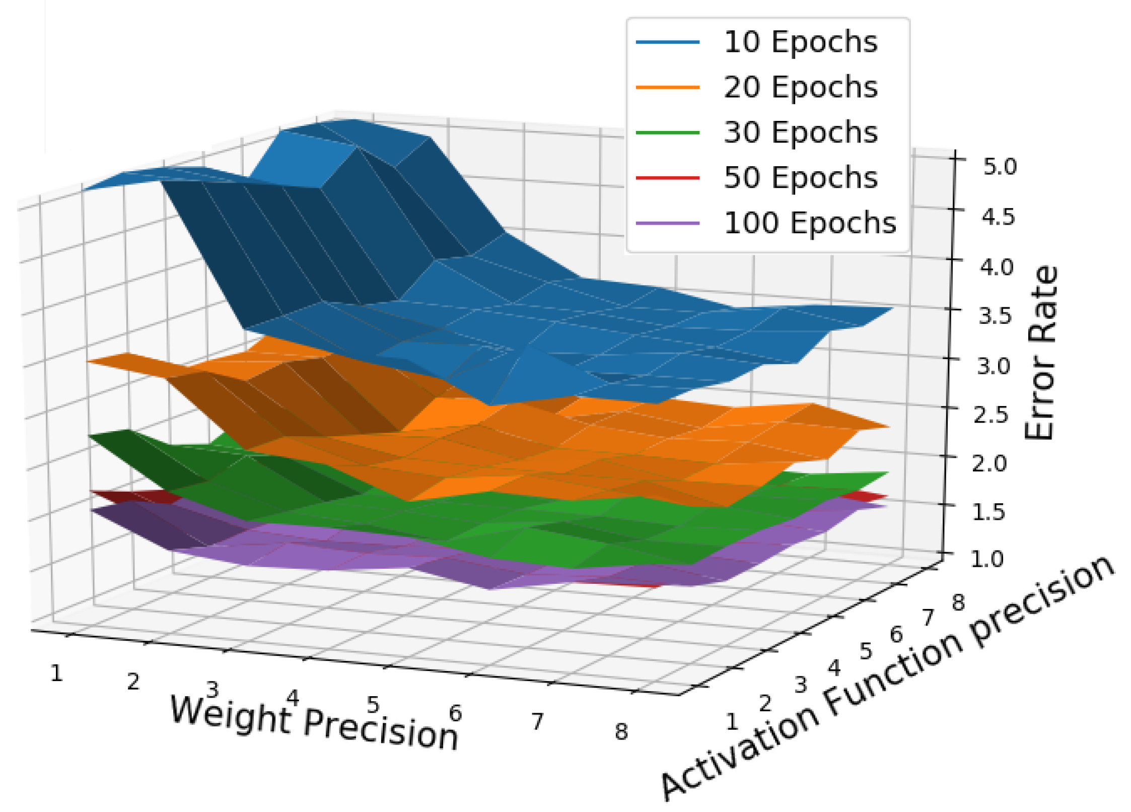
  • Inference accuracy is highest with higher precision, i.e., least aggressive quantisation. The biggest improvement in accuracy with a 1 bit increment is switching from 1 to 2 bits weight precision.
  • With enough training beyond 50 epochs, 2 bit precision achieves almost the same inference accuracy as 3–8 bit precision.
  • Increasing the parallelisation of hardware neural network implementations significantly increases throughput performance from 6.1 k FPS to 373 k FPS, a 62 × speedup.
  • The trade-off between precision, throughput and accuracy is the W3A3 model with 16 for PE and SIMD, achieving 373 k FPS and 85.5% accuracy for the FASHION-MNIST dataset.

4.3. NEMOKD Results

For the NEMOKD experiments in this section, we used two student models as our solution space for hyper-parameter evolution:
  • FlexStudent, a model that we constructed with a simple five layer model to provide a starting point for the NEMOKD evolution process (Section 3). A similar model performs well as a student architecture on the CIFAR10 dataset [33].
  • A version of the Resnet8x4 architecture, modified to enable the NEMOKD hyper-parameter evolutionary process.
Our NEMOKD framework was measured with three benchmarks:
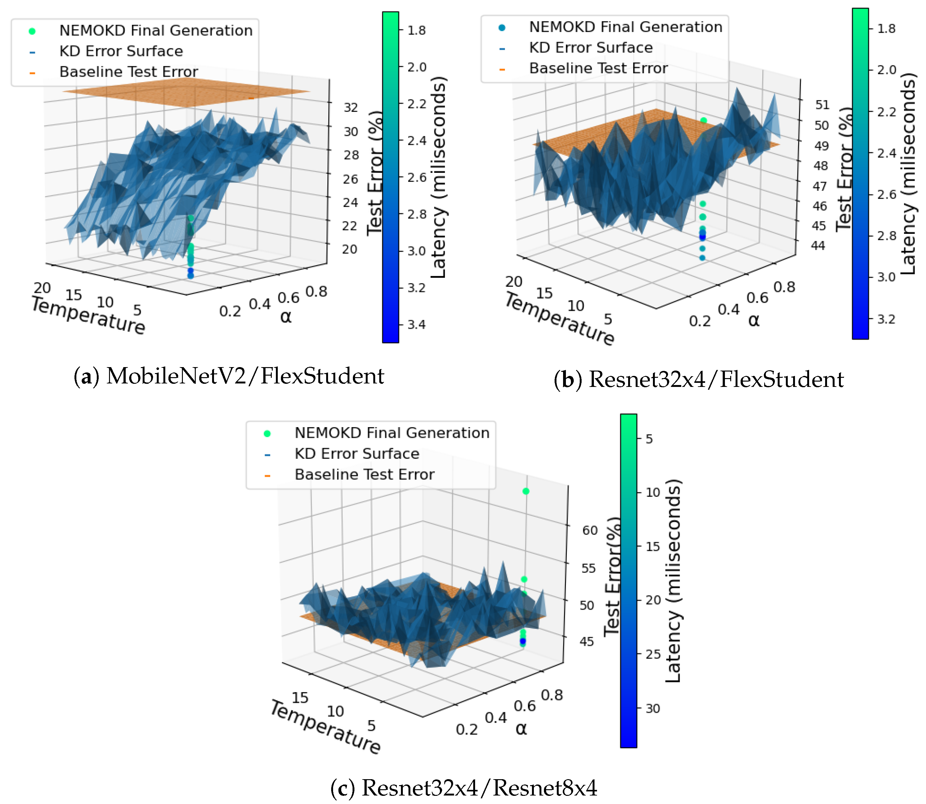
  • The MobileNetV2 model distilled into a FlexStudent student model with the CIFAR10 dataset.
  • The Resnet32x4 model distilled into a FlexStudent student model with CIFAR100.
  • The Resnet32x4 model distilled into a Resnet8x4 student model with CIFAR100. For this experiment, the number of layers remained fixed.
The experiments used 30 epochs for knowledge distillation and the number of NSGAII generations varies for each experiment, ranging from 14 to 27. For our pruning benchmarks we used Platypus [34] for multi-objective optimisation, RepDistiller [35] for knowledge distillation, and OpenVino’s Python API to execute trained exported PyTorch models on the NSC2 device.

4.3.1. Knowledge Distillation Parameter Search

Figure 9 shows knowledge distillation error with 30 epochs. It illustrates how different combinations of knowledge distillation parameters affected the accuracy of the baseline model after 30 epochs. The α value determined how much the distillation loss and student loss contributed to the overall loss e.g., if α = 0.5 , then both terms in the knowledge distillation loss function were weighted evenly. The softmax function in the distillation loss term was parametrised by the temperature. This softened the output distribution revealing extra information about which classes the model found most alike. The blue surface illustrates the error rate of the baseline model with respect to different combinations of knowledge distillation hyper-parameters. The orange plane indicates the baseline test error performance without knowledge distillation.
For the MobileNetV2 teacher, a FlexStudent student model and CIFAR10 in Figure 9a, any choice of knowledge distillation hyper-parameters provided a significant increase in accuracy over the baseline model.
Figure 9b shows that some combinations of the knowledge distillation parameters had a negative effect on the accuracy of the baseline model. We observed that this method produced better accuracy than could be obtained by distilling knowledge into the baseline model, once again at the expense of latency. The MobileNetV2/FlexStudent experiment in Figure 9a is similar to Figure 9b, but rather than CIFAR100 it used the simpler CIFAR10 dataset. In this case, every combination of knowledge distillation hyper parameters provided significant improvement over baseline.
In Figure 9c, the majority of combinations of knowledge distillation hyper-parameters had a negative impact on the baseline model accuracy, though certain combinations did provide improvements as shown in Figure 9c. In this case, no major trends were observed with respect to the individual hyper-parameters. We observed that this method, once again, produced better accuracy than could be obtained by distilling knowledge into the baseline model with 30 epochs of training.

4.3.2. Efficacy of NEMOKD Evolution

Figure 10 shows the latency and accuracy performance of student models after 30 epochs for student models. It shows the baseline model trained with just knowledge distillation (green diamonds). The red and blue points show performance of the models at intermediate and final generations of student models. As with the quantisation experiments, accuracy was measured using a testing dataset to asses how the models generalised to new unseen data.
Figure 10a shows FlexStudent student performance with the MobileNetV2 teacher. The chosen knowledge distillation hyper-parameters for this experiment greatly increased the accuracy of the baseline model. With 30 epochs of training, many students in the final generation evolved to attain a better accuracy than the baseline model but with the same or better latency. The same was also true of the baseline model trained with knowledge distillation. The most accurate students, however, had larger latency values with respect to the baseline model. The best latency/accuracy trade-off for Resnet32x4/FlexStudent distillation with CIFAR10 was an evolved model with five convolutional layers with a relatively small number of output channels and just two fully connected layers. It has a low to moderate number of neurons of about 125–150 neurons.
Figure 10b shows FlexStudent student performance with the larger Resnet32x4 teacher model, for the CIFAR100 dataset. Student models evolved from the same baseline FlexStudent as the experiment in Figure 10a. Figure 10b illustrates the population at two distinct generations of the evolutionary process, in addition to the baseline architecture from which all the students evolved. Interestingly, the combination of knowledge distillation hyper-parameters we chose for this experiment had a negative impact on the accuracy of the baseline model. However, the evolved students appeared to adapt their architecture to accommodate these parameters, resulting in student models with significant accuracy improvements for the same inference latency. The best accuracy produced by the NEMOKD algorithm was obtained by an architecture with a higher latency. In contrast to Figure 10a, every student model in the final generation evolved to have the same layer structure as the baseline model.
Figure 10c shows Resnet8x4 student performance student performance with the Resnet32x4 teacher, for the CIFAR100 dataset. It differs from Figure 10a,b in two ways: (1) a different evolutionary starting point is used for the ResNet8x4 student; and (2) the layers of this student model are fixed, only the output channels of the convolutional layers were modified in the NEMOKD evolutionary process.

4.4. Discussion

4.4.1. Quantisation for FPGAs

Our quantisation experiments (Section 4.2) use the quantisation scheme implemented in Xilinx’s FINN framework. Developing compression algorithms for embedded devices is a research area of its own, e.g., a dynamic precision data quantisation algorithm in [36], performed layer-by-layer from a corresponding floating point CNN, with the goal of improving bandwidth and resource utilisation. Other compression approaches are focused on specific goals e.g., reducing power consumption, or target specific hardware e.g., GPUs or FPGAs, or target specific domains or even specific application algorithms.

Device Specific Quantisation

Recent work explores the performance trade-offs between reduced precision of neural networks and their speed on GPUs, e.g., performance aware pruning can lead to 3–10 times speedups [37]. Multi-precision FPGA hardware for neural networks significantly reduces model sizes, which in [38] enables an ImageNet network to fit entirely on-chip for the first time, significantly speeding up throughput. Another recent study [25] measures the hardware cost, power consumption, and throughput for a High Level Synthesis extension of FINN that supports Long Short-Term Memory (LSTM) models on FPGAs. [39] proposes a design flow for constructing low precision, low powered FPGA-based neural networks with a hybrid quantisation scheme. [40] shows that resource-aware model analysis, data quantisation and efficient use of hardware techniques can be combined to jointly map binarised neural networks to FPGAs with dramatically reduced resource requirements whilst maintaining acceptable accuracy.

Domain Specific Quantisation

Some quantisation methods target specific algorithms, e.g., a resource-aware weight quantisation framework for performing object detection in images [41].

4.4.2. NEMO with Knowledge Distillation for the VPU

Knowledge distillation parameters for the NEMOKD experiments (Section 4.3) greatly increase the accuracy of the baseline model. With 30 epochs of training, many students in the final generation evolve to attain a better accuracy than the baseline model but with the same or better latency. The most accurate students, however, have larger latency values with respect to the baseline model. The best trade-off model evolved five convolutional layers with a small number of output channels and just two fully connected layers, with a low to moderate number of neurons of about 125–150 neurons.
Our NEMOKD approach significantly increases inference accuracy at a modest expense of latency. The method consistently provides higher accuracy students than could be obtained through an exhaustive knowledge distillation parameter search with the baseline model, irrespective of the choice of knowledge distillation hyper-parameters. This highlights the importance of the student’s architecture in the knowledge distillation process. Evolving students appears to enable models to adapt and accommodate an arbitrary choice of knowledge distillation hyper-parameters, even if the choice was initially detrimental to the accuracy of the baseline model.

4.4.3. Comparing Quantisation and NEMOKD

The quantisation and NEMOKD results are shown in Figure 11. Both compression approaches start from baseline models: ResNet32x4 and MobileNetV2 for NEMOKD, and a 32 bit Multi-Layer Perceptron model for quantisation. Quantisation reduces the arithmetic precision without changing a model’s architecture, i.e., the number of hidden layers and number of neurons are unchanged. Training with the FINN framework is quantisation-aware, with performance sweet spots for our benchmarks at around 2–4 bits.
In contrast, the NEMOKD framework changes the model’s architecture whilst leaving arithmetic precision unchanged during training. After training, models are converted into the OpenVINO IR format with 16-bit half precision for deployment on the VPU.
Typically, 30 image FPS throughput is considered real-time computer vision performance [42]. Quantisation and the NEMOKD framework both achieve real-time image processing: 590 FPS on the VPU and 373 k FPS on the FPGA.

5. Conclusions and Future Work

5.1. Conclusions

This paper explores two optimisation approaches for neural networks for programmable hardware and a fixed AI processor: (1) quantisation precision of fixed models, and (2) evolving hyper-parameters of student models in conjunction with knowledge distillation. There is a sweet spot of 3 bit quantisation in the trade-off between latency, hardware requirements, training time and accuracy. Parallelising hardware implementations of neural networks increases FPS from 6 k to 373 k, a 62 × speedup. Evolving student models increases inference accuracy by up to 82% at the cost of 38% increased latency. The lowest inference latencies were 1.7 ms for the FlexStudent model distilled from MobileNetV2, 1.4 ms for FlexStudent distilled from Resnet32x4, and 2 ms for Resnet8x4 distilled from Resnet32x4. This is a throughput of between 100 and 590 FPS.

5.2. Future Work

5.2.1. Larger Datasets and Models

Our experiments use four datasets: MNIST and FASHION-MNIST for quantisation, and CIFAR10 and CIFAR100 for NEMOKD. The quantisation experiments are based on a five layer fully-connected network and the NEMOKD experiments use two student models. More work is required to scale accuracy-preserving compression methods to real world computer vision applications e.g., from 28 × 28 MNIST and FASHION-MNIST images, and 32 × 32 CIFAR10 and CIFAR100 images, to much higher dimensions such as 400 × 150 road lane detection images for autonomous driving [43]. Scaling compressing experiments to (1) deeper models with tens/hundreds of hidden layers, and (2) datasets with thousands of classes e.g., ImageNet, would be an intermediate step in that direction.

5.2.2. Profile Guided Automating Compression

Our quantisation benchmarks were exhaustive in the design space of 1–8 bits for activation functions and weight values. The quantisation was homogeneous across the entire network each time, i.e., each quantisation configuration applied to all parameters. Combining layer-specific dataflow optimisation and layer-specific quantisation allows models to fit entirely in on-chip BRAM, thereby removing off-chip memory accesses which improves throughput performance [44]. In [45], mixed precision quantisation scheme applies layer-wise priority in inverse order of their layer depth, based on findings that binarising different layers has a widely-varied effect on accuracy loss. FINN supports per-layer activation function and weights precision, as well as layer-by-layer clock cycle profiling and accuracy testing. This opens up the opportunity for automating profile guided layer-by-layer quantisation methodologies in simulation i.e., without having to run models on hardware, to find the optimal trade-off between throughput and accuracy for each combination of model and dataset.
When using evolutionary algorithms with knowledge distillation for larger datasets and models, enabling more parameters to be the subject of mutation throughout the evolutionary process could prove beneficial in automating search for optimal compressed models. Recent teacher-student methods [35] outperform knowledge distillation in a wide range of problems. Designing a flexible student model that accommodates both evolution and more complex distillation methods would be considerably more challenging, but given the positive results we report for NEMOKD we believe this would be important future work.

5.2.3. Performance Portability of Compressed Models

The two compression methods in this paper were tested on one hardware platform each. Our NEMOKD approach is hardware-aware, since the multi-objective optimisation phase is measured on the Intel Movidius VPU device. Evolving the same initial model with the goal of minimising latency and accuracy loss may produce quite different models for different devices due to different memory latencies, cache size and the number of parallel processing elements on each device. For quantisation, the amount of on-chip BRAM memory ranges from 0.5 to 8 MB for different FPGA devices, meaning aggressive quantisation and binarisation is needed for low-end devices, necessitating auto-tuning of model precision to be device specific.

5.2.4. Combining Knowledge Distillation with Quantisation

Previous work shows that combining compression methods can achieve superior performance compared with using them in isolation, e.g., combining pruning and knowledge distillation [46]. The approach in [47] shows that distilling knowledge to shallower quantised architectures can achieve accuracy comparable with state-of-the-art full-precision models. There are other compression methods such as weight sharing [48] to consider for hybrid compression. A complete study of neural network compression approaches is in [21].
More work is required to evaluate these hybrid neural network compression techniques at the scale of state-of-the-art real world problems. Not only may hybrid methods achieve superior throughput performance and energy efficiency, reducing precision and removing unimportant redundancy at scale may make verification of large real-world deep learning models possible.

Author Contributions

The individual contributions are as follows. R.S.: conceptualisation; funding acquisition; investigation; project administration; resources; supervision; writing—original draft; writing—review and editing. P.B.: software Section 2; data curation Section 4.2; visualisation Section 4.2; formal analysis Section 4.4; writing—original draft preparation Section 2.1 and Section 4.2. Q.D.: software Section 2; data curation Section 4.2.3; visualisation Section 4.2.3; writing—original draft preparation Section 4.2.3. A.N.: conceptualization Section 3; software Section 3; data curation Section 4.3; formal analysis Section 4.3; visualisation Section 4.3; writing—original draft preparation Section 3 and Section 4.3. E.K.: funding acquisition; supervision; writing—review and editing. All authors have read and agreed to the published version of the manuscript.

Funding

This research was funded by EPSRC project “Border Patrol: Improving Smart Device Security through Type-Aware Systems Design (EP/N028201/1)”; EPSRC project “Serious Coding: A Game Approach To Security For The New Code-Citizens (EP/T017511/1)”; National Cyber Security Center, UK, Grant “SecConn-NN: Neural Networks with Security Contracts—towards lightweight, modular security for neural networks”; UK Research Institute in Verified Trustworthy Software Systems research project “CONVENER: Continuous Verification of Neural Networks” (from the “Digital Security Through Verification” call).

Conflicts of Interest

The authors declare no conflict of interest.

References

  1. Krizhevsky, A.; Sutskever, I.; Hinton, G.E. ImageNet Classification with Deep Convolutional Neural Networks. In Proceedings of the Advances in Neural Information Processing Systems 25: 26th Annual Conference on Neural Information Processing Systems 2012, Lake Tahoe, NV, USA, 3–6 December 2012; pp. 1106–1114. [Google Scholar]
  2. Lu, D. Creating an AI Can Be Five Times Worse for the Planet Than a Car. New Scientist. 2019. Available online: https://www.newscientist.com/article/2205779-creating-an-ai-can-be-five-times-worse-for-the-planet-than-a-car (accessed on 28 December 2020).
  3. Intel. Intel® Movidius™ Vision Processing Units (VPUs). Available online: https://www.intel.com/content/www/us/en/products/processors/movidius-vpu.html (accessed on 28 December 2020).
  4. Edge TPU: Google’s Purpose-Built ASIC Designed to Run Inference at the Edge. Available online: https://cloud.google.com/edge-tpu (accessed on 28 December 2020).
  5. Véstias, M.P.; Neto, H.C. Trends of CPU, GPU and FPGA for high-performance computing. In Proceedings of the 2014 24th International Conference on Field Programmable Logic and Applications (FPL), Munich, Germany, 2–4 September 2014; pp. 1–6. [Google Scholar]
  6. Han, S.; Pool, J.; Tran, J.; Dally, W.J. Learning both Weights and Connections for Efficient Neural Network. In Proceedings of the Advances in Neural Information Processing Systems 28: Annual Conference on Neural Information Processing Systems 2015, Montreal, QC, Canada, 7–12 December 2015; pp. 1135–1143. [Google Scholar]
  7. Umuroglu, Y.; Fraser, N.J.; Gambardella, G.; Blott, M.; Leong, P.H.W.; Jahre, M.; Vissers, K.A. FINN: A Framework for Fast, Scalable Binarized Neural Network Inference. In Proceedings of the 2017 ACM/SIGDA International Symposium on Field-Programmable Gate, Monterey, CA, USA, 22–24 February 2017; pp. 65–74. [Google Scholar]
  8. Hinton, G.E.; Vinyals, O.; Dean, J. Distilling the Knowledge in a Neural Network. arXiv 2015, arXiv:1503.02531. [Google Scholar]
  9. Diamos, G.; Sengupta, S.; Catanzaro, B.; Chrzanowski, M.; Coates, A.; Elsen, E.; Engel, J.H.; Hannun, A.Y.; Satheesh, S. Persistent RNNs: Stashing Recurrent Weights On-Chip. In Proceedings of the 33nd International Conference on Machine Learning (ICML 2016), New York, NY, USA, 19–24 June 2016; Volume 48, pp. 2024–2033. [Google Scholar]
  10. Chen, T.; Du, Z.; Sun, N.; Wang, J.; Wu, C.; Chen, Y.; Temam, O. DianNao: A small-footprint high-throughput accelerator for ubiquitous machine-learning. In Proceedings of the ASPLOS 2014, Salt Lake City, UT, USA, 1–5 March 2014; pp. 269–284. [Google Scholar]
  11. Park, J.; Sung, W. FPGA based implementation of deep neural networks using on-chip memory only. In Proceedings of the ICASSP 2016, Shanghai, China, 20–25 March 2016; pp. 1011–1015. [Google Scholar]
  12. Katz, G.; Barrett, C.W.; Dill, D.L.; Julian, K.; Kochenderfer, M.J. Reluplex: An Efficient SMT Solver for Verifying Deep Neural Networks. In Proceedings of the Computer Aided Verification-29th International Conference (CAV 2017), Heidelberg, Germany, 24–28 July 2017; pp. 97–117. [Google Scholar]
  13. Liu, C.; Arnon, T.; Lazarus, C.; Barrett, C.W.; Kochenderfer, M.J. Algorithms for Verifying Deep Neural Networks. arXiv 2019, arXiv:1903.06758. [Google Scholar]
  14. Kokke, W.; Komendantskaya, E.; Kienitz, D.; Atkey, R.; Aspinall, D. Neural Networks, Secure by Construction: An Exploration of Refinement Types. In Asian Symposium on Programming Languages and Systems (APLAS), Fukuoka, Japan; Springer: Berlin/Heidelberg, Germany, 2020. [Google Scholar]
  15. Duncan, K.; Komendantskaya, E.; Stewart, R.; Lones, M.A. Relative Robustness of Quantized Neural Networks against Adversarial Attacks. In Proceedings of the 2020 International Joint Conference on Neural Networks (IJCNN 2020), Glasgow, UK, 19–24 July 2020; pp. 1–8. [Google Scholar]
  16. Lecun, Y.; Bottou, L.; Bengio, Y.; Haffner, P. Gradient-based learning applied to document recognition. Proc. IEEE 1998, 86, 2278–2324. [Google Scholar] [CrossRef] [Green Version]
  17. Szegedy, C.; Ioffe, S.; Vanhoucke, V.; Alemi, A.A. Inception-v4, Inception-ResNet and the Impact of Residual Connections on Learning. In Proceedings of the Thirty-First AAAI Conference on Artificial Intelligence, San Francisco, CA, USA, 4–9 February 2017; pp. 4278–4284. [Google Scholar]
  18. Zhang, X.; Li, Z.; Loy, C.C.; Lin, D. PolyNet: A Pursuit of Structural Diversity in Very Deep Networks. In Proceedings of the 2017 IEEE Conference on Computer Vision and Pattern Recognition (CVPR 2017), Honolulu, HI, USA, 21–26 July 2017; pp. 3900–3908. [Google Scholar]
  19. Tan, M.; Le, Q.V. EfficientNet: Rethinking Model Scaling for Convolutional Neural Networks. In Proceedings of the 36th International Conference on Machine Learning (ICML 2019), Long Beach, CA, USA, 9–15 June 2019; pp. 6105–6114. [Google Scholar]
  20. Mahajan, D.; Girshick, R.B.; Ramanathan, V.; He, K.; Paluri, M.; Li, Y.; Bharambe, A.; van der Maaten, L. Exploring the Limits of Weakly Supervised Pretraining. arXiv 2018, arXiv:1805.00932. [Google Scholar]
  21. Wang, E.; Davis, J.J.; Zhao, R.; Ng, H.; Niu, X.; Luk, W.; Cheung, P.Y.K.; Constantinides, G.A. Deep Neural Network Approximation for Custom Hardware: Where We’ve Been, Where We’re Going. ACM Comput. Surv. 2019, 52, 40:1–40:39. [Google Scholar] [CrossRef] [Green Version]
  22. Hubara, I.; Courbariaux, M.; Soudry, D.; El-Yaniv, R.; Bengio, Y. Quantized Neural Networks: Training Neural Networks with Low Precision Weights and Activations. J. Mach. Learn. Res. 2017, 18, 187:1–187:30. [Google Scholar]
  23. Courbariaux, M.; Bengio, Y. BinaryNet: Training Deep Neural Networks with Weights and Activations Constrained to +1 or −1. arXiv 2016, arXiv:1602.02830. [Google Scholar]
  24. Blott, M.; Preußer, T.B.; Fraser, N.J.; Gambardella, G.; O’Brien, K.; Umuroglu, Y.; Leeser, M.; Vissers, K.A. FINN-R: An End-to-End Deep-Learning Framework for Fast Exploration of Quantized Neural Networks. TRETS 2018, 11, 16:1–16:23. [Google Scholar] [CrossRef]
  25. Rybalkin, V.; Pappalardo, A.; Ghaffar, M.M.; Gambardella, G.; Wehn, N.; Blott, M. FINN-L: Library Extensions and Design Trade-Off Analysis for Variable Precision LSTM Networks on FPGAs. In Proceedings of the FPL 2018, Dublin, Ireland, 27–31 August 2018; pp. 89–96. [Google Scholar]
  26. Stanley, K.O.; Miikkulainen, R. Evolving Neural Networks through Augmenting Topologies. Evol. Comput. 2002, 10, 99–127. [Google Scholar] [CrossRef] [PubMed]
  27. Dong, J.; Cheng, A.; Juan, D.; Wei, W.; Sun, M. DPP-Net: Device-Aware Progressive Search for Pareto-Optimal Neural Architectures. In Proceedings of the Computer Vision-ECCV 2018-15th European Conference, Munich, Germany, 8–14 September 2018; pp. 540–555. [Google Scholar]
  28. Huang, G.; Liu, S.; van der Maaten, L.; Weinberger, K.Q. CondenseNet: An Efficient DenseNet Using Learned Group Convolutions. In Proceedings of the 2018 IEEE Conference on Computer Vision and Pattern Recognition, CVPR 2018, Salt Lake City, UT, USA, 18–22 June 2018; pp. 2752–2761. [Google Scholar]
  29. Kim, Y.H.; Reddy, B.; Yun, S.; Seo, C. NEMO: Neuro-Evolution with Multiobjective Optimization of Deep Neural Network for Speed and Accuracy. In Proceedings of the AutoML 2017: Automatic Machine Learning Workshop (ICML 2017), Sydney, Australia, 10 August 2017. [Google Scholar]
  30. Zmora, N.; Jacob, G.; Zlotnik, L.; Elharar, B.; Novik, G. Neural Network Distiller: A Python Package For DNN Compression Research. arXiv 2019, arXiv:1910.12232. [Google Scholar]
  31. Deb, K.; Agrawal, S.; Pratap, A.; Meyarivan, T. A fast and elitist multiobjective genetic algorithm: NSGA-II. IEEE Trans. Evol. Comput. 2002, 6, 182–197. [Google Scholar] [CrossRef] [Green Version]
  32. Su, J.; Fraser, N.J.; Gambardella, G.; Blott, M.; Durelli, G.; Thomas, D.B.; Leong, P.H.W.; Cheung, P.Y.K. Accuracy to Throughput Trade-Offs for Reduced Precision Neural Networks on Reconfigurable Logic. In Proceedings of the ARC 2018, Santorini, Greece, 2–4 May 2018; pp. 29–42. [Google Scholar]
  33. Exploring Knowledge Distillation of Deep Neural Nets for Efficient Hardware Solutions. CS230 Report. Available online: http://cs230.stanford.edu/files_winter_2018/projects/6940224.pdf (accessed on 28 December 2020).
  34. Hadka, D. Platypus: Multiobjective Optimization in Python. Available online: https://platypus.readthedocs.io (accessed on 28 December 2020).
  35. Tian, Y.; Krishnan, D.; Isola, P. Contrastive Representation Distillation. In Proceedings of the 8th International Conference on Learning Representations (ICLR 2020), Addis Ababa, Ethiopia, 26–30 April 2020. [Google Scholar]
  36. Qiu, J.; Wang, J.; Yao, S.; Guo, K.; Li, B.; Zhou, E.; Yu, J.; Tang, T.; Xu, N.; Song, S.; et al. Going Deeper with Embedded FPGA Platform for Convolutional Neural Network. In Proceedings of the 2016 ACM/SIGDA International Symposium on Field-Programmable Gate Arrays, Monterey, CA, USA, 21–23 February 2016; pp. 26–35. [Google Scholar]
  37. Radu, V.; Kaszyk, K.; Wen, Y.; Turner, J.; Cano, J.; Crowley, E.J.; Franke, B.; Storkey, A.; O’Boyle, M. Performance Aware Convolutional Neural Network Channel Pruning for Embedded GPUs. In Proceedings of the 2019 IEEE International Symposium on Workload Characterization (IISWC), Orlando, FL, USA, 3–5 November 2019. [Google Scholar]
  38. Zhao, Y.; Gao, X.; Guo, X.; Liu, J.; Wang, E.; Mullins, R.; Cheung, P.Y.K.; Constantinides, G.A.; Xu, C. Automatic Generation of Multi-Precision Multi-Arithmetic CNN Accelerators for FPGAs. In Proceedings of the 2019 International Conference on Field-Programmable Technology (ICFPT), Tianjin, China, 9–13 December 2019; pp. 45–53. [Google Scholar]
  39. Wang, J.; Lou, Q.; Zhang, X.; Zhu, C.; Lin, Y.; Chen, D. Design Flow of Accelerating Hybrid Extremely Low Bit-Width Neural Network in Embedded FPGA. In Proceedings of the FPL 2018, Dublin, Ireland, 27–31 August 2018; pp. 163–169. [Google Scholar]
  40. Liang, S.; Yin, S.; Liu, L.; Luk, W.; Wei, S. FP-BNN: Binarized neural network on FPGA. Neurocomputing 2018, 275, 1072–1086. [Google Scholar] [CrossRef]
  41. Ding, C.; Wang, S.; Liu, N.; Xu, K.; Wang, Y.; Liang, Y. REQ-YOLO: A Resource-Aware, Efficient Quantization Framework for Object Detection on FPGAs. In Proceedings of the FPGA 2019, Seaside, CA, USA, 24–26 February 2019; pp. 33–42. [Google Scholar]
  42. Gu, Q.; Ishii, I. Review of some advances and applications in real-time high-speed vision: Our views and experiences. Int. J. Autom. Comput. 2016, 13, 305–318. [Google Scholar] [CrossRef]
  43. Cheng, C.H. Towards Robust Direct Perception Networks for Automated Driving. In Proceedings of the 2020 IEEE Intelligent Vehicles Symposium (IV), Las Vegas, NV, USA, 19 October–13 November 2020. [Google Scholar]
  44. Nguyen, D.T.; Kim, H.; Lee, H. Layer-specific Optimization for Mixed Data Flow with Mixed Precision in FPGA Design for CNN-based Object Detectors. IEEE Trans. Circuits Syst. Video Technol. 2020. [Google Scholar] [CrossRef]
  45. Wang, H.; Xu, Y.; Ni, B.; Zhuang, L.; Xu, H. Flexible Network Binarization with Layer-Wise Priority. In Proceedings of the 2018 25th IEEE International Conference on Image Processing (ICIP), Athens, Greece, 7–10 October 2018; pp. 2346–2350. [Google Scholar]
  46. Turner, J.; Crowley, E.J.; Radu, V.; Cano, J.; Storkey, A.; O’Boyle, M. Distilling with Performance Enhanced Students. arXiv 2018, arXiv:1810.10460. [Google Scholar]
  47. Polino, A.; Pascanu, R.; Alistarh, D. Model compression via distillation and quantization. In Proceedings of the 6th International Conference on Learning Representations (ICLR 2018), Vancouver, BC, Canada, 30 April–3 May 2018. [Google Scholar]
  48. Cheng, Y.; Yu, F.X.; Feris, R.S.; Kumar, S.; Choudhary, A.N.; Chang, S. Fast Neural Networks with Circulant Projections. arXiv 2015, arXiv:1502.03436. [Google Scholar]
Figure 1. Meeting in the middle: compressing neural networks for acceleration.
Electronics 10 00396 g001
Figure 2. Hyperbolic tangent with different quantisation configuration.
Electronics 10 00396 g002
Figure 3. Decoding the genotype representation of the baseline FlexStudent.
Electronics 10 00396 g003
Figure 4. NEMOKD methodology.
Electronics 10 00396 g004
Figure 5. Accuracy of Quantised Neural Networks (QNN) with increasing training.
Electronics 10 00396 g005
Figure 6. Hardware resources required for 64 quantised neural networks.
Electronics 10 00396 g006
Figure 7. Radar charts for different quantisation configurations.
Electronics 10 00396 g007
Figure 8. Throughput and accuracy performance of parallel FPGA designs for FASHION-MNIST.
Electronics 10 00396 g008
Figure 9. Knowledge distillation parameter search for Teacher/Student distillation.
Electronics 10 00396 g009
Figure 10. Student latency and accuracy performance for Teacher/Student distillation.
Electronics 10 00396 g010
Figure 11. Varying precision and model architectures.
Electronics 10 00396 g011
Table 1. Quantised weight values between 0.136 and 2 with m i n = 2 and m a x = 2 .
ValuePrecision (bits)
12345678
0.1361000.250.1250.1250.1250.140625
0.357100.50.250.3750.3750.343750.359375
0.639110.50.750.6250.6250.6250.640625
1.1351111.251.1251.1251.1251.140625
2111.51.751.8751.93751.968751.984375
Table 2. Quantisation and model evolution experiments
DeviceModelDatasetSection
Xilinx Z7020 FPGA3 layer fully connected MLPMNISTSection 4.2.1 and Section 4.2.2
(quantisation)3 layer fully connected MLPFASHION-MNISTSection 4.2.3
Intel Movidius Myriad X VPUTeacherStudent
MobileNetV2FlexStudentCIFAR10Section 4.3
(model evolution)Resnet32x4FlexStudentCIFAR100Section 4.3
Resnet32x4Resnet8x4CIFAR100Section 4.3
Table 3. Relative performance for radar plots in Figure 7.
MetricRelative Performance
WorstBest
Accuracy loss2.07%1.52%
BRAM1643224
Flip Flops226,28231,954
Look Up Tables223,91053,336
Publisher’s Note: MDPI stays neutral with regard to jurisdictional claims in published maps and institutional affiliations.

