
Channel Impulse Response at 60 GHz and Impact of Electrical Parameters Properties on Ray Tracing Validations

 ,
, 

 ,
, 
Abstract
1. Introduction
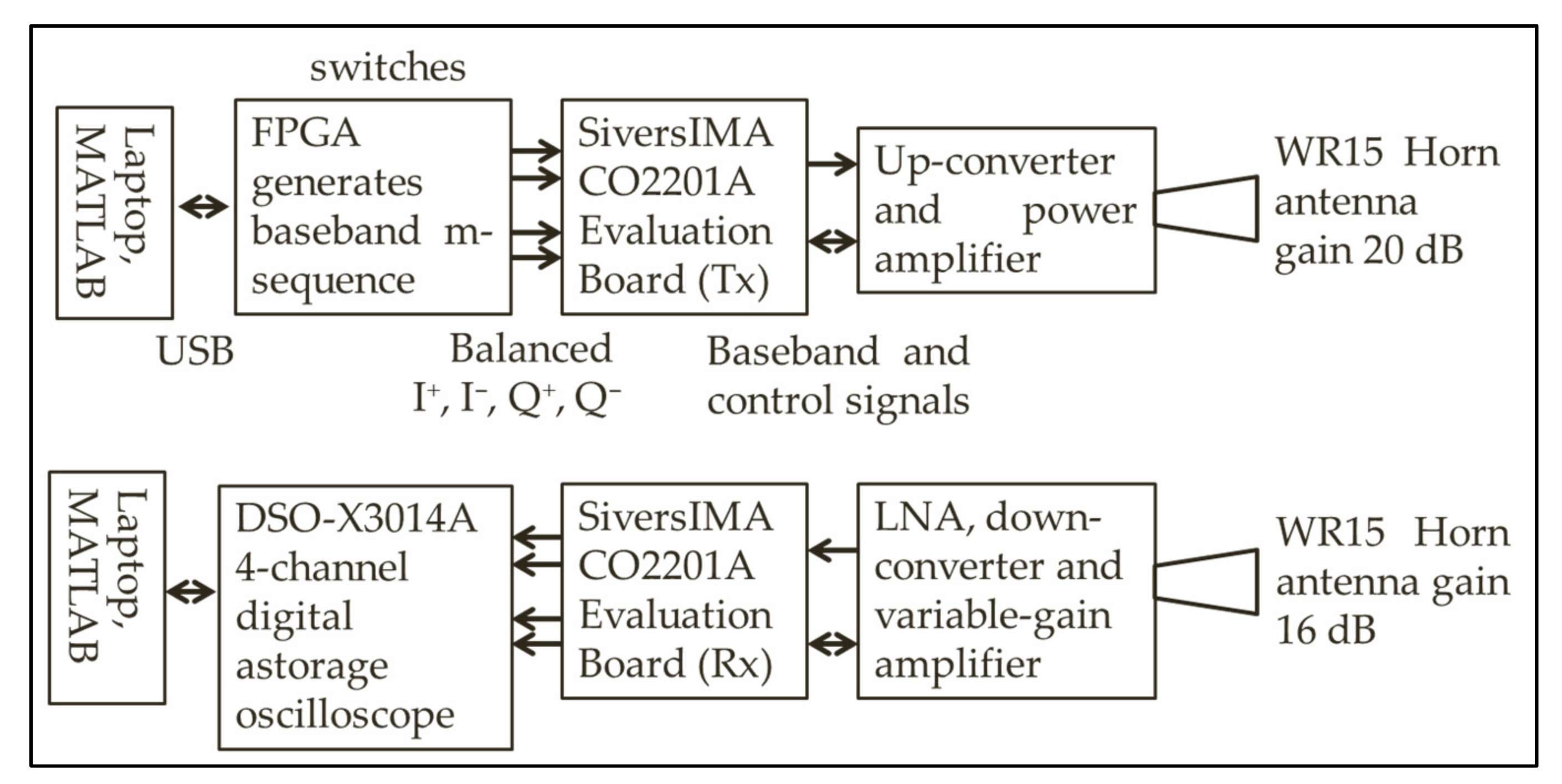
2. Channel Sounder
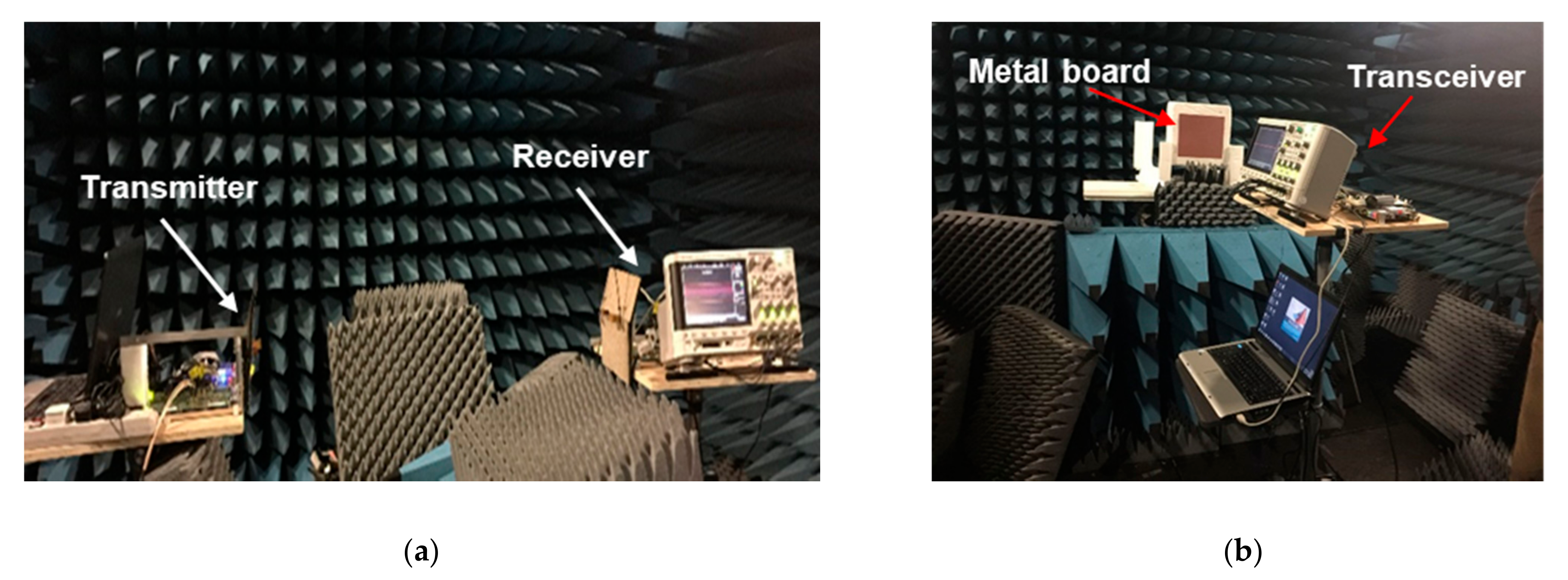
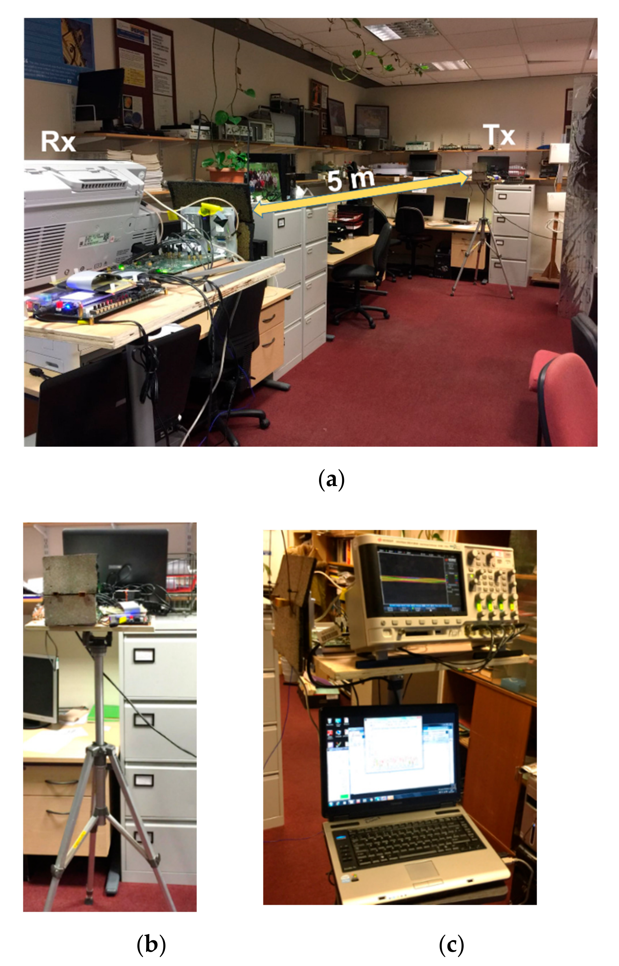
3. Experimental Setup
3.1. LOS Experiment
3.2. NLOS Experiment
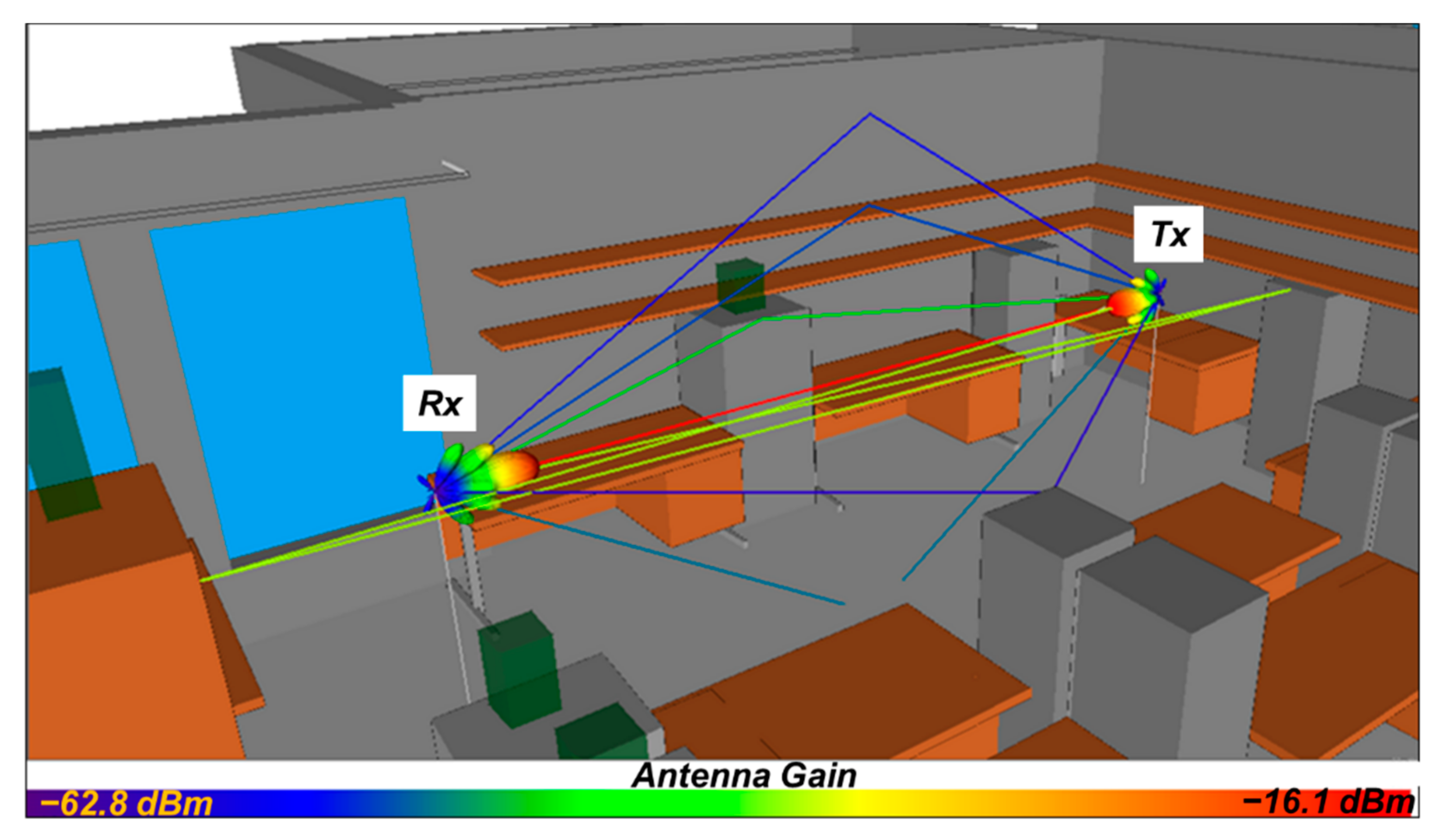
4. Results and Discussion
4.1. LOS Scenario
4.2. NLOS Scenario
4.2.1. Position 1
4.2.2. Position 2
- Case 1: LOS for (120–180°) rotation
- Case 2: Reflection from a wooden board for 210–250° rotations
4.2.3. Position 3: (Reflection on Two Wooden Surfaces)
5. Conclusions
Author Contributions
Funding
Data Availability Statement
Conflicts of Interest
References
- Nitsche, T.; Cordeiro, C.; Flores, A.B.; Knightly, E.W.; Perahia, E.; Widmer, J.C. IEEE 802.11 ad: Directional 60 GHz communication for multi-Gigabit-per-second Wi-Fi. IEEE Commun. Mag. 2014, 52, 132–141. [Google Scholar] [CrossRef]
- Yilmaz, T.; Fadel, E.; Akan, O.B. Employing 60 GHz ISM Band for 5G Wireless Communications. In Proceedings of the 2014 IEEE International Black Sea Conference on Communications and Networking (BlackSeaCom), Chisinau, Moldova, 27–30 May 2014; IEEE: New York, NY, USA, 2014; pp. 77–82. [Google Scholar]
- Roh, W.; Seol, J.-Y.; Park, J.; Lee, B.; Lee, J.; Kim, Y.; Cho, J.; Cheun, K.; Aryanfar, F. Millimeter-wave beamforming as an enabling technology for 5G cellular communications: Theoretical feasibility and prototype results. IEEE Commun. Mag. 2014, 52, 106–113. [Google Scholar] [CrossRef]
- Cordeiro, C. The pursuit of tens of gigabits per second wireless systems [Industry Perspectives]. IEEE Wirel. Commun. 2013, 20, 3–5. [Google Scholar] [CrossRef]
- Guo, N.; Qiu, R.C.; Mo, S.S.; Takahashi, K. 60-GHz millimeter-wave radio: Principle, technology, and new results. EURASIP J. Wirel. Commun. Netw. 2006, 2007, 68253. [Google Scholar] [CrossRef][Green Version]
- Liu, P.; Di Renzo, M.; Springer, A. Line-of-sight spatial modulation for indoor mmWave communication at 60 GHz. IEEE Trans. Wirel. Commun. 2016, 15, 7373–7389. [Google Scholar] [CrossRef]
- Rappaport, T.S.; Heath, R.W., Jr.; Daniels, R.C.; Murdock, J.N. Millimeter Wave Wireless Communications; Pearson Education: New York, NY, USA, 2015; ISBN 0132172283. [Google Scholar]
- Hansen, C.J. WiGiG: Multi-gigabit wireless communications in the 60 GHz band. IEEE Wirel. Commun. 2011, 18, 6–7. [Google Scholar] [CrossRef]
- Saha, S.K.; Ghasempour, Y.; Haider, M.K.; Siddiqui, T.; De Melo, P.; Somanchi, N.; Zakrajsek, L.; Singh, A.; Shyamsunder, R.; Torres, O. X60: A programmable testbed for wideband 60 ghz wlans with phased arrays. Comput. Commun. 2019, 133, 77–88. [Google Scholar] [CrossRef]
- Pang, J.; Maki, S.; Kawai, S.; Nagashima, N.; Seo, Y.; Dome, M.; Kato, H.; Katsuragi, M.; Kimura, K.; Kondo, S. A 50.1-Gb/s 60-GHz CMOS transceiver for IEEE 802.11 ay with calibration of LO feedthrough and I/Q imbalance. IEEE J. Solid State Circuits 2019, 54, 1375–1390. [Google Scholar] [CrossRef]
- Ghasempour, Y.; da Silva, C.R.C.M.; Cordeiro, C.; Knightly, E.W. IEEE 802.11 ay: Next-generation 60 GHz communication for 100 Gb/s Wi-Fi. IEEE Commun. Mag. 2017, 55, 186–192. [Google Scholar] [CrossRef]
- Wu, X.; Wang, C.-X.; Sun, J.; Huang, J.; Feng, R.; Yang, Y.; Ge, X. 60-GHz millimeter-wave channel measurements and modeling for indoor office environments. IEEE Trans. Antennas Propag. 2017, 65, 1912–1924. [Google Scholar] [CrossRef]
- AlAbdullah, A.A.; Ali, N.; Obeidat, H.; Abd-Alhmeed, R.A.; Jones, S. Indoor Millimetre-Wave Propagation Channel Simulations at 28, 39, 60 and 73 GHz for 5G Wireless Networks. In Proceedings of the 2017 Internet Technologies and Applications (ITA), North East Wales, UK, 12–15 September 2017; IEEE: New York, NY, USA, 2017; pp. 235–239. [Google Scholar]
- Saha, S.K.; Vira, V.V.; Garg, A.; Koutsonikolas, D. A feasibility study of 60 GHz indoor WLANs. In Proceedings of the 2016 25th International Conference on Computer Communication and Networks (ICCCN), Waikoloa, HI, USA, 1–4 August 2016; IEEE: New York, NY, USA, 2016; pp. 1–9. [Google Scholar]
- Saha, S.K.; Malleshappa, D.G.; Palamanda, A.; Vira, V.V.; Garg, A.; Koutsonikolas, D. 60 GHz indoor WLANs: Insights into performance and power consumption. Wirel. Netw. 2018, 24, 2427–2450. [Google Scholar] [CrossRef]
- Salous, S.; Gao, Y. Wideband Measurements in Indoor and Outdoor Environments in the 30 GHz and 60 GHz Bands. In Proceedings of the 2016 10th European Conference on Antennas and Propagation (EuCAP), Davos, Switzerland, 10–15 April 2016; IEEE: New York, NY, USA, 2016; pp. 1–3. [Google Scholar]
- Rangan, S.; Rappaport, T.S.; Erkip, E. Millimeter-wave cellular wireless networks: Potentials and challenges. Proc. IEEE 2014, 102, 366–385. [Google Scholar] [CrossRef]
- Sulyman, A.I.; Seleem, H.; Alwarafy, A.; Humadi, K.M.; Alsanie, A. Effects of solar radio emissions on outdoor propagation path loss models at 60 GHz bands for access/backhaul links and D2D communications. IEEE Trans. Antennas Propag. 2017, 65, 6624–6635. [Google Scholar] [CrossRef]
- Diakhate, C.A.L.; Conrat, J.-M.; Cousin, J.-C.; Sibille, A. Millimeter-Wave Outdoor-to-Indoor Channel Measurements at 3, 10, 17 and 60 GHz. In Proceedings of the 2017 11th European Conference on Antennas and Propagation (EUCAP), Paris, France, 19–24 March 2017; IEEE: New York, NY, USA, 2017; pp. 1798–1802. [Google Scholar]
- Manan, W.; Obeidat, H.; Al-Abdullah, A.; Abd-Alhameed, R.; Hu, F. Indoor to indoor and indoor to outdoor millimeter wave propagation channel simulations at 26 Ghz, 28 Ghz and 60 Ghz for 5G mobile networks. Int. J. Eng. Sci 2018, 7, 8–18. [Google Scholar]
- Obeidat, H.; Alabdullah, A.; Elkhazmi, E.; Suhaib, W.; Obeidat, O.; Alkhambashi, M.; Mosleh, M.; Ali, N.; Dama, Y.; Abidin, Z.; et al. Indoor environment propagation review. Comput. Sci. Rev. 2020, 37, 100272. [Google Scholar] [CrossRef]
- Medeđović, P.; Veletić, M.; Blagojević, Ž. Wireless insite software verification via analysis and comparison of simulation and measurement results. In Proceedings of the 2012 35th International Convention MIPRO, Opatija, Croatia, 21–25 May 2012; pp. 776–781. [Google Scholar]
- Obeidat, H.A.; Obeidat, O.A.; Mosleh, M.F.; Abdullah, A.A.; Abd-Alhameed, R.A. Verifying Received Power Predictions of Wireless InSite Software in Indoor Environments at WLAN Frequencies. Appl. Comput. Electromagn. Soc. J. 2020, 35, 1119–1126. [Google Scholar] [CrossRef]
- Dama, Y.A.S.; Abd-Alhameed, R.A.; Salazar-Quinonez, F.; Zhou, D.; Jones, S.M.R.; Gao, S. MIMO Indoor Propagation Prediction Using 3D Shoot-and-Bounce Ray (SBR) Tracing Technique for 2.4 GHz and 5 GHz. In Proceedings of the 5th European Conference on Antennas and Propagation (EUCAP), Rome, Italy, 11–15 April 2011; IEEE: New York, NY, USA, 2011; pp. 1655–1658. [Google Scholar]
- Remcom. Wireless InSite Reference Manual, 3.1.0; Remcom: State College, PA, USA, 2017. [Google Scholar]
- Balanis, C.A. Antenna Theory: Analysis and Design; John Wiley & Sons: Hoboken, NJ, USA, 2016; ISBN 1118642066. [Google Scholar]
- Series, P. Effects of building materials and structures on radiowave propagation above about 100 MHz. Recomm. ITU-R 2015, 2040–2041. Available online: https://www.itu.int/dms_pubrec/itu-r/rec/p/R-REC-P.2040-1-201507-I!!PDF-E.pdf (accessed on 1 December 2020).
- Correia, L.M.; Frances, P.O. Transmission and isolation of signals in buildings at 60 GHz. Proceedings of 6th International Symposium on Personal, Indoor and Mobile Radio Communications, Toronto, ON, Canada, 27–29 September 1995; Volume 3, p. 1031. [Google Scholar]
- Pinhasi, Y.; Yahalom, A.; Petnev, S. Propagation of ultra wide-band signals in lossy dispersive media. In Proceedings of the 2008 IEEE International Conference on Microwaves, Communications, Antennas and Electronic Systems, Tel Aviv, Israel, 13–14 May 2008; pp. 1–10. [Google Scholar]
- Stavrou, S.; Saunders, S.R. Review of Constitutive Parameters of Building Materials. In Proceedings of the Twelfth International Conference on Antennas and Propagation, 2003 (ICAP 2003), Exeter, UK, 31 March–3 April 2003; IET: London, UK, 2003; Volume 1, pp. 211–215. [Google Scholar]
- Torgovnikov, G.I. Dielectric Properties of Wood and Wood-Based Materials; Springer: Berlin/Heidelberg, Germany, 1993. [Google Scholar]
- Series, P. Propagation data and prediction methods for the planning of indoor radiocommunication systems and radio local area networks in the frequency range 900 MHz to 100 GHz. Recomm. ITU-R 2012, 1237–1238. Available online: https://www.itu.int/dms_pubrec/itu-r/rec/p/R-REC-P.1238-8-201507-S!!PDF-E.pdf (accessed on 1 December 2020).
- Fares, M.; Fargier, Y.; Villain, G.; Derobert, X.; Lopes, S.P. Determining the permittivity profile inside reinforced concrete using capacitive probes. NDT E Int. 2016, 79, 150–161. [Google Scholar] [CrossRef]
- Fakharzadeh, M.; Nezhad-Ahmadi, M.-R.; Biglarbegian, B.; Ahmadi-Shokouh, J.; Safavi-Naeini, S. CMOS phased array transceiver technology for 60 GHz wireless applications. IEEE Trans. Antennas Propag. 2010, 58, 1093–1104. [Google Scholar] [CrossRef]
- Lu, J.; Steinbach, D.; Cabrol, P.; Pietraski, P.; Pragada, R.V. Propagation Characterization of An Office Building in the 60 GHz Band. In Proceedings of the 8th European Conference on Antennas and Propagation (EuCAP 2014), The Hague, The Netherlands, 6–11 April 2014; IEEE: New York, NY, USA, 2014; pp. 809–813. [Google Scholar]
- Correia, L.M.; Frances, P.O. Transmission and isolation of signals in buildings at 60 GHz. In Proceedings of the 6th International Symposium on Personal, Indoor and Mobile Radio Communications, Helsinki, Finland, 13–16 September 2021; IEEE: New York, NY, USA, 1995; Volume 3, p. 1031. [Google Scholar]
- Affum, E.; Tchao, E.T.; Diawuo, K.; Agyekum, K. Wideband Parameters Analysis and Validation for Indoor radio Channel at 60/70/80 GHz for Gigabit Wireless Communication employing Isotropic, Horn and Omni directional Antenna. arXiv 2013, arXiv:1312.5109. [Google Scholar] [CrossRef][Green Version]
- Salous, S.; Degli Esposti, V.; Fuschini, F.; Thomae, R.S.; Mueller, R.; Dupleich, D.; Haneda, K.; Garcia-Pardo, J.-M.M.; Garcia, J.P.; Gaillot, D.P. Millimeter-Wave Propagation: Characterization and modeling toward fifth-generation systems. [Wireless Corner]. IEEE Antennas Propag. Mag. 2016, 58, 115–127. [Google Scholar] [CrossRef]


| Item | Value |
|---|---|
| Internal pulse amplitude | 5 V peak |
| Bit period | 4 ns |
| Bandwidth of operation | 400 MHz |
| EIRP * | 32 dBm |
| Data rate | 250 bps |
| sampling interval | 2 ns |
| Sweep speed | 10 µs/div |
| HPBW * E (dB) | 18.72° |
| HPBW H (dB) | 23.03° |
| Material | Reference | εr | σ | Description |
|---|---|---|---|---|
| Concrete | [32] (a) | 5.31 | 0.897 | ITU-A |
| [32] (b) | 6.5 | 0.228 | ITU-B | |
| [33] | 7–13 | - | Fares | |
| [34] | 6.13 | 1.005 | Fakharzadeh | |
| [35] | 3.3 | 1.267 | Lu | |
| [36] (a) | 6.14 | 1.005 | Correia-A | |
| [36] (b) | 6.5 | 1.428 | Correia-B | |
| [29] | 11.47 | 0.988 | Pinhasi | |
| Wood | [32] | 1.99 | 0.378 | ITU |
| [31] | 2.1 | 0.2 | Torgovnikov | |
| [34] | 1.57 | 0.321 | Fakharzadeh | |
| [37] | 3.3 | - | Affum | |
| [35] | 2.8 | 0.001 | Lu | |
| [36] (a) | 1.57 | 0.321 | Correia-A | |
| [36] (b) | 1.54 | 0.118 | Correia-B | |
| [38] | 2.4 | 0.4 | Salous | |
| [29] (a) | 1.64 | 3.717 | Pinhasi-A | |
| [29] (b) | 2.068 | 1.38 | Pinhasi-B |
| Receiver | Measured | Simulated |
|---|---|---|
| Rx2_120 | −42.89 | −51.742 |
| Rx2_130 | −33.82 | −46.533 |
| Rx2_140 | −23.86 | −34.464 |
| Rx2_150 | −24.16 | −28.308 |
| Rx2_160 | −25.78 | −30.812 |
| Rx2_170 | −52.46 | −41.34 |
| Rx2_180 | −50.37 | −48.37 |
| Receiver | Measured | [33] + [32] (a) | [32] (a) | [32] (b) | [34] | [35] | [36] (a) | [36] (b) | [29] |
|---|---|---|---|---|---|---|---|---|---|
| Rx2_120 | −58.53 | −63.45 | −69.61 | −67.90 | −68.36 | −74.76 | −68.35 | −67.87 | −64.12 |
| Rx2_130 | −54.30 | −63.97 | −70.13 | −68.42 | −68.88 | −75.28 | −68.87 | −68.39 | −64.64 |
| Rx2_140 | −54.98 | −53.36 | −59.51 | −57.81 | −58.26 | −64.66 | −58.25 | −57.78 | −54.02 |
| Rx2_150 | −40.34 | −48.39 | −54.60 | −52.89 | −53.35 | −59.75 | −53.34 | −52.86 | −49.11 |
| Rx2_160 | −37.92 | −35.65 | −41.81 | −40.10 | −40.56 | −46.96 | −40.55 | −40.07 | −36.32 |
| Rx2_170 | −39.38 | −31.34 | −37.50 | −35.79 | −36.24 | −42.65 | −36.23 | −35.76 | −32.01 |
| Rx2_180 | −46.20 | −35.01 | −35.50 | −39.44 | −39.89 | −46.30 | −39.88 | −39.41 | −35.66 |
| RMSE | 7.3694 | 10.2147 | 8.5859 | 8.8307 | 13.4507 | 8.8252 | 8.5706 | 7.4062 | |
| Rotations | ||
|---|---|---|
| Rx3_150° | Rx3_160° | |
| Measured | −37.11 | −52.14 |
| [32] (a) | −50.05 | −49.03 |
| [31] | −48.73 | −47.72 |
| [34] | −54.60 | −53.60 |
| [37] + [32] (a) | −44.70 | −43.70 |
| [35] | −37.25 | −39.77 |
| [36] (a) | −54.55 | −53.54 |
| [36] (b) | −56.93 | −55.91 |
| [38] | −47.70 | −46.69 |
| [29] (a) | −46.80 | −45.79 |
| [29] (b) | −48.94 | −47.93 |
Publisher’s Note: MDPI stays neutral with regard to jurisdictional claims in published maps and institutional affiliations. |
© 2021 by the authors. Licensee MDPI, Basel, Switzerland. This article is an open access article distributed under the terms and conditions of the Creative Commons Attribution (CC BY) license (http://creativecommons.org/licenses/by/4.0/).
Share and Cite
Obeidat, H.; Ullah, A.; AlAbdullah, A.; Manan, W.; Obeidat, O.; Shauieb, W.; Dama, Y.; Kara-Zaïtri, C.; Abd-Alhameed, R. Channel Impulse Response at 60 GHz and Impact of Electrical Parameters Properties on Ray Tracing Validations. Electronics 2021, 10, 393. https://doi.org/10.3390/electronics10040393
Obeidat H, Ullah A, AlAbdullah A, Manan W, Obeidat O, Shauieb W, Dama Y, Kara-Zaïtri C, Abd-Alhameed R. Channel Impulse Response at 60 GHz and Impact of Electrical Parameters Properties on Ray Tracing Validations. Electronics. 2021; 10(4):393. https://doi.org/10.3390/electronics10040393
Chicago/Turabian StyleObeidat, Huthaifa, Atta Ullah, Ali AlAbdullah, Waqas Manan, Omar Obeidat, Wafa Shauieb, Yousef Dama, Chakib Kara-Zaïtri, and Raed Abd-Alhameed. 2021. "Channel Impulse Response at 60 GHz and Impact of Electrical Parameters Properties on Ray Tracing Validations" Electronics 10, no. 4: 393. https://doi.org/10.3390/electronics10040393
APA StyleObeidat, H., Ullah, A., AlAbdullah, A., Manan, W., Obeidat, O., Shauieb, W., Dama, Y., Kara-Zaïtri, C., & Abd-Alhameed, R. (2021). Channel Impulse Response at 60 GHz and Impact of Electrical Parameters Properties on Ray Tracing Validations. Electronics, 10(4), 393. https://doi.org/10.3390/electronics10040393