Review

The Impact of State-of-the-Art Techniques for Lossless Still Image Compression

School of Computer Science and Engineering, The University of Aizu, Aizu-Wakamatsu City, Fukushima 965-8580, Japan
*
Authors to whom correspondence should be addressed.
Electronics 2021, 10(3), 360; https://doi.org/10.3390/electronics10030360
Submission received: 3 January 2021 / Revised: 21 January 2021 / Accepted: 28 January 2021 / Published: 2 February 2021
(This article belongs to the Special Issue Recent Advances in Multimedia Signal Processing and Communications)

Abstract

:
A great deal of information is produced daily, due to advances in telecommunication, and the issue of storing it on digital devices or transmitting it over the Internet is challenging. Data compression is essential in managing this information well. Therefore, research on data compression has become a topic of great interest to researchers, and the number of applications in this area is increasing. Over the last few decades, international organisations have developed many strategies for data compression, and there is no specific algorithm that works well on all types of data. The compression ratio, as well as encoding and decoding times, are mainly used to evaluate an algorithm for lossless image compression. However, although the compression ratio is more significant for some applications, others may require higher encoding or decoding speeds or both; alternatively, all three parameters may be equally important. The main aim of this article is to analyse the most advanced lossless image compression algorithms from each point of view, and evaluate the strength of each algorithm for each kind of image. We develop a technique regarding how to evaluate an image compression algorithm that is based on more than one parameter. The findings that are presented in this paper may be helpful to new researchers and to users in this area.

1. Introduction

A huge amount of data is now produced daily, especially in medical centres and on social media. It is not easy to manage these increasing quantities of information, which are impractical to store and they take a huge amount of time to transmit over the Internet. More than 2.5 quintillion bytes of data are produced daily, and this figure is growing, according to the sixth edition of a report by DOMO [1]. The report further estimates that approximately 90% of the world’s data were produced between 2018 and 2019, and that each person on earth will create 1.7 MB of data per second by 2020. Consequently, storing large amounts of data on digital devices and quickly transferring them across networks is a significant challenge. There are three possible solutions to this problem: better hardware, better software, or a combination of both. However, so much information is being created that it is almost impossible to design new hardware that is sufficiently competitive, due to the many limitations on the construction of hardware, as reported in [2]. Therefore, the development of better software is the only solution to the problem.
One solution from the software perspective is compression. Data compression is a way of representing data using fewer bits than the original in order to reduce the consumption of storage and bandwidth and increase transmission speed over networks [3]. Data compression can be applied in many areas, such as audio, video, text, and images, and it can be classified into two categories: lossless and lossy [4]. In lossy compression, irrelevant and less significant data are removed permanently, whereas, in lossless compression, every detail is preserved and only statistical redundancy is eliminated. In short, lossy compression allows for slight degradation in the data, while lossless methods perfectly reconstruct the data from its compressed form [5,6,7,8]. There are many applications for lossless data compression techniques, such as medical imagery, digital radiography, scientific imaging, zip file compression, museums/art galleries, facsimile transmissions of bitonal images, business documents, machine vision, the storage and sending of thermal images taken by nano-satellites, observation of forest fires, etc. [9,10,11,12,13]. In this article, we study the compression standards that are used for lossless image compression. There are many such methods, including run-length coding, Shannon–Fano coding, Lempel–Ziv–Welch (LZW) coding, Huffman coding, arithmetic coding, lossless JPEG, PNG, JPEG 2000, JPEG-LS, JPGE XR, CALIC, AVIF, WebP, FLIF, etc. However, we limit our analysis to lossless JPEG, PNG, JPEG 2000, JPEG-LS, JPGE XR, CALIC, AVIF, WebP, and FLIF, since these are the latest and most fully developed methods in this area. Although there are also many types of image, such as binary images, 8-bit and 16-bit grayscale images, 8-bit indexed images, and 8-bit and 16-bit red, green, and blue (RGB) images, we only cover 8-bit and 16-bit grayscale and RGB images in this article. A detailed review of run-length, Shannon–Fano, LZW, Huffman, and arithmetic coding was carried out in [3]. Four parameters are used to evaluate a lossless image compression algorithm: the compression ratio (CR), bits per pixel (bpp), encoding time (ET), and decoding time (DT), and bpp is the simply the inverse of the CR; therefore, we only consider the CR, ET, and DT when evaluating these methods. Most studies in this research area use only the CR to evaluate the effectiveness of an algorithm [14,15,16,17]. Although there are many applications for which higher CRs are important, others may require higher encoding or decoding speeds. Other applications may require high CR and low ET, low ET and DT, or high CR and decoding speed. In addition, there are also many applications where all three of these parameters are equally important. In view of this, we present an extensive analysis from each perspective, and then examine the strength of each algorithm for each kind of image. We compare the performance of these methods based on public open datasets. More specifically, the main aim of this research is to address the following research issues:
RI1:
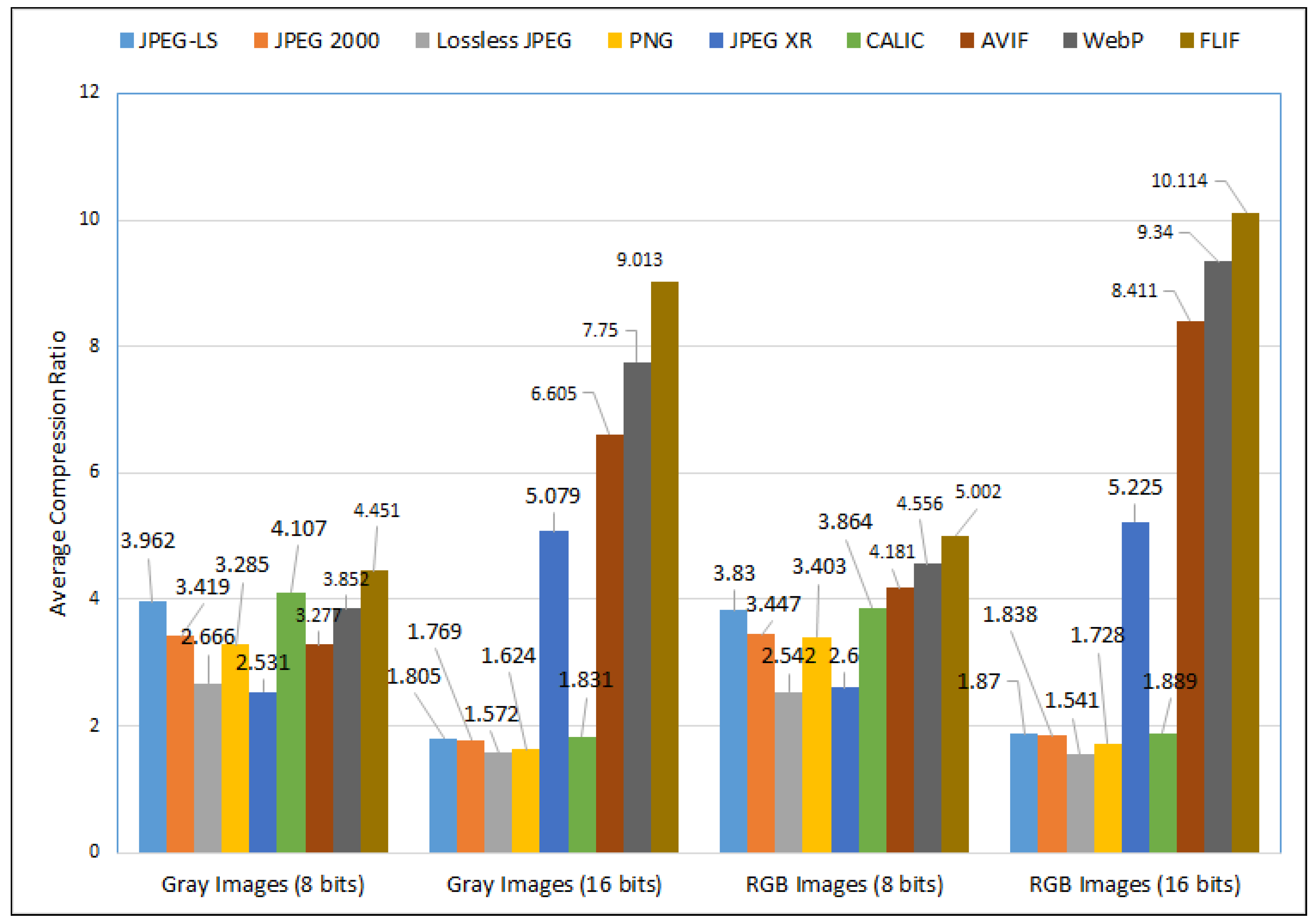
How good is each algorithm in terms of the CR for 8-bit and 16-bit greyscale and RGB images?
RI2:
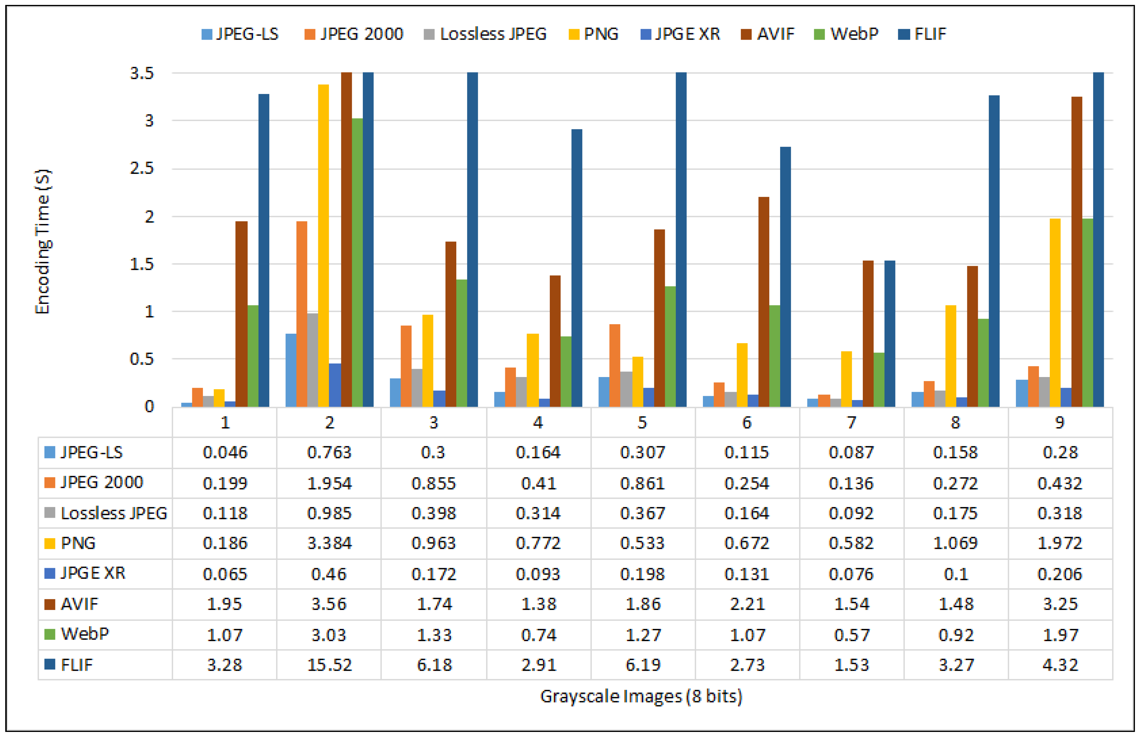
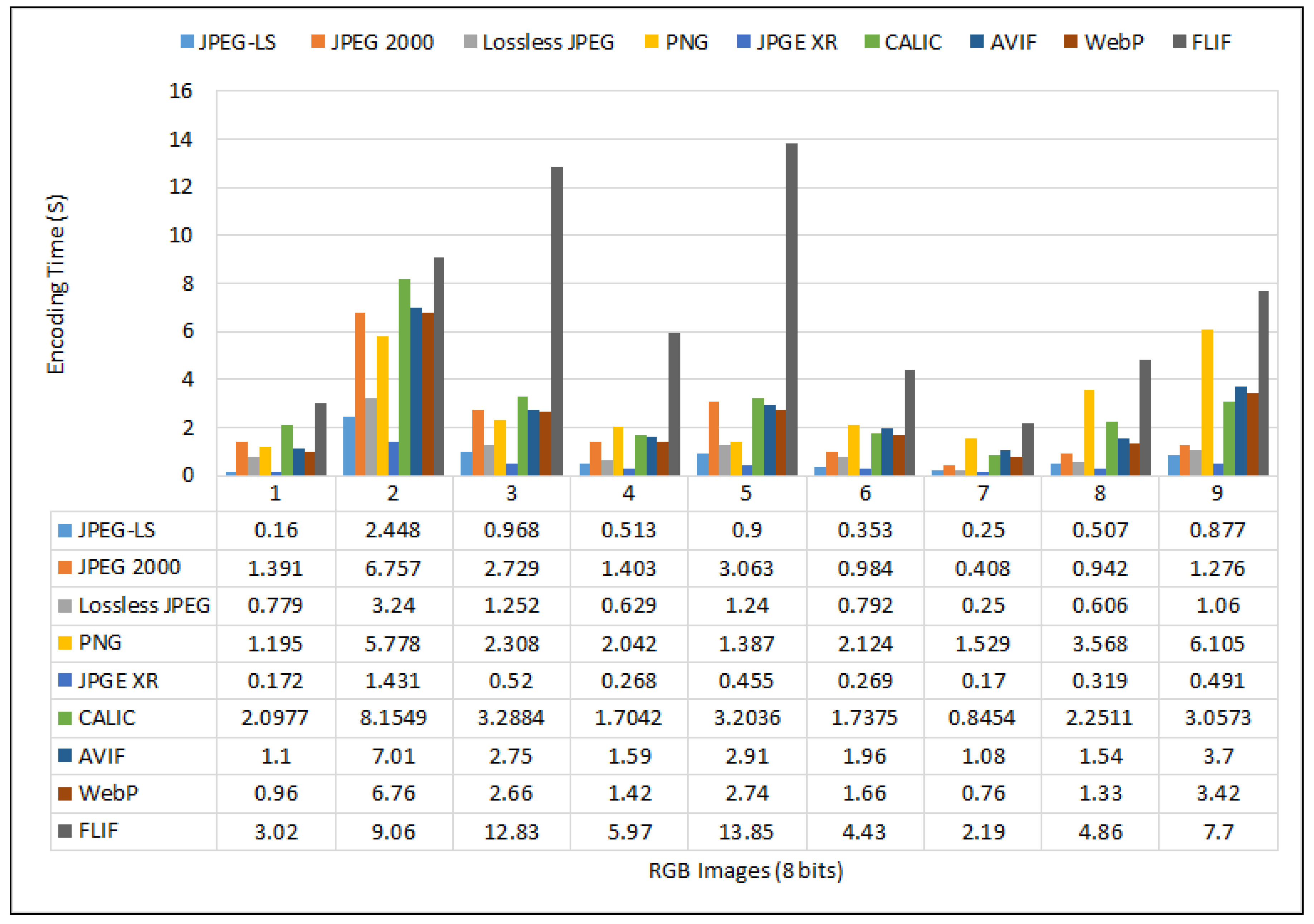
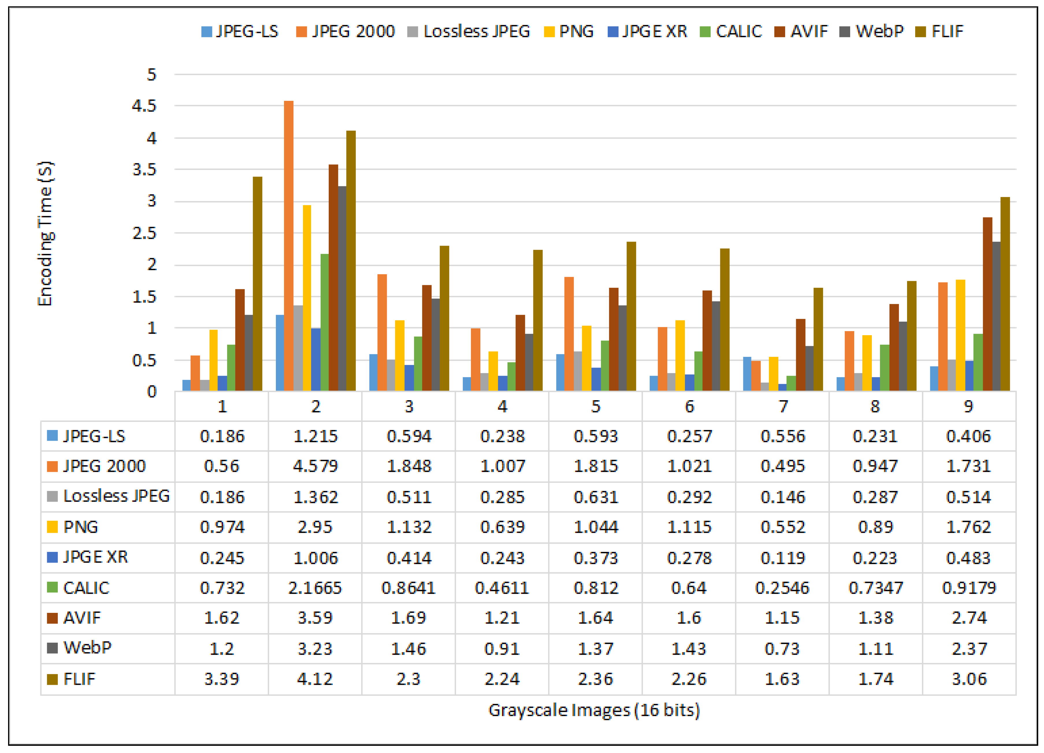
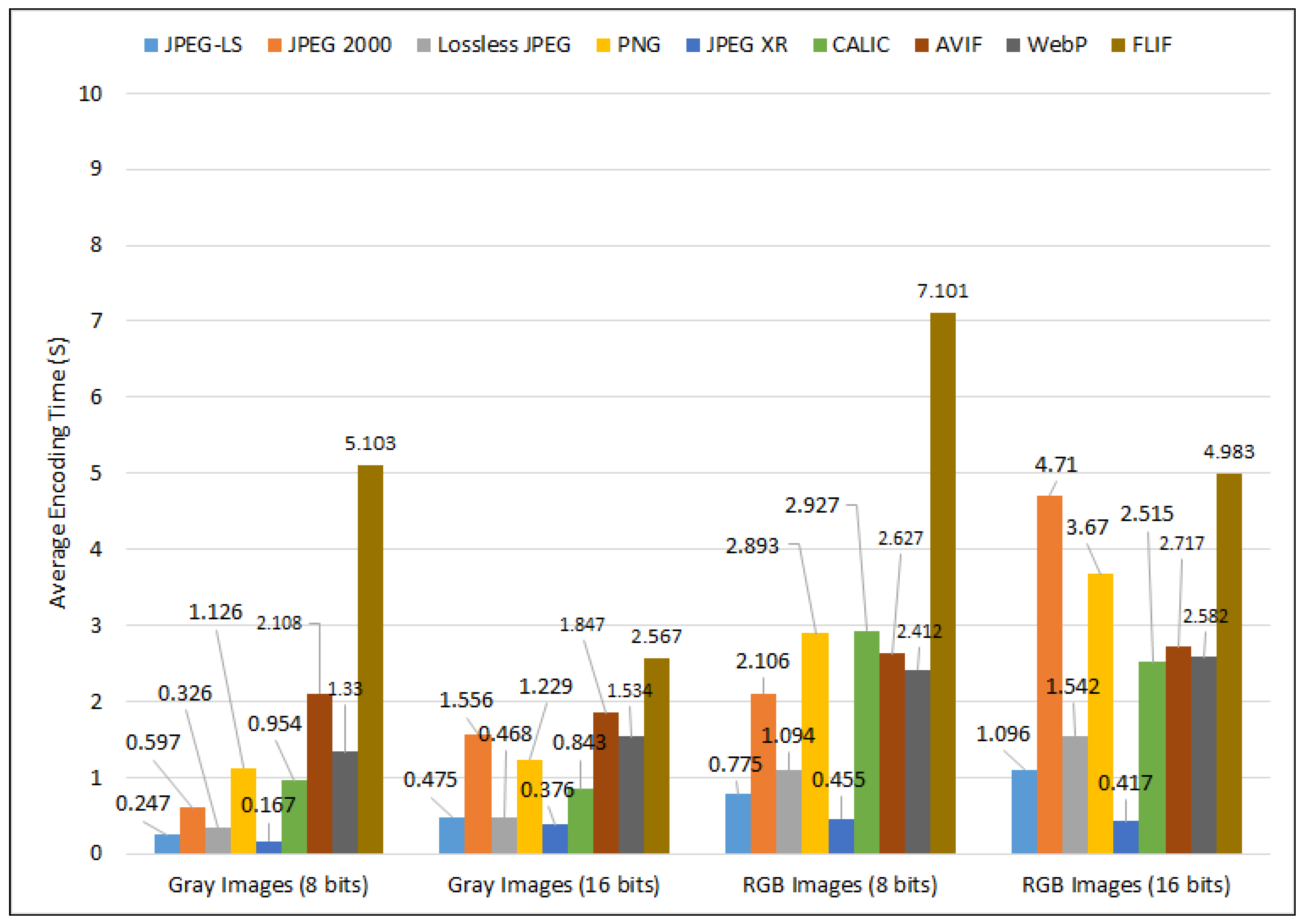
How good is each algorithm in terms of the ET for 8-bit and 16-bit greyscale and RGB images?
RI3:
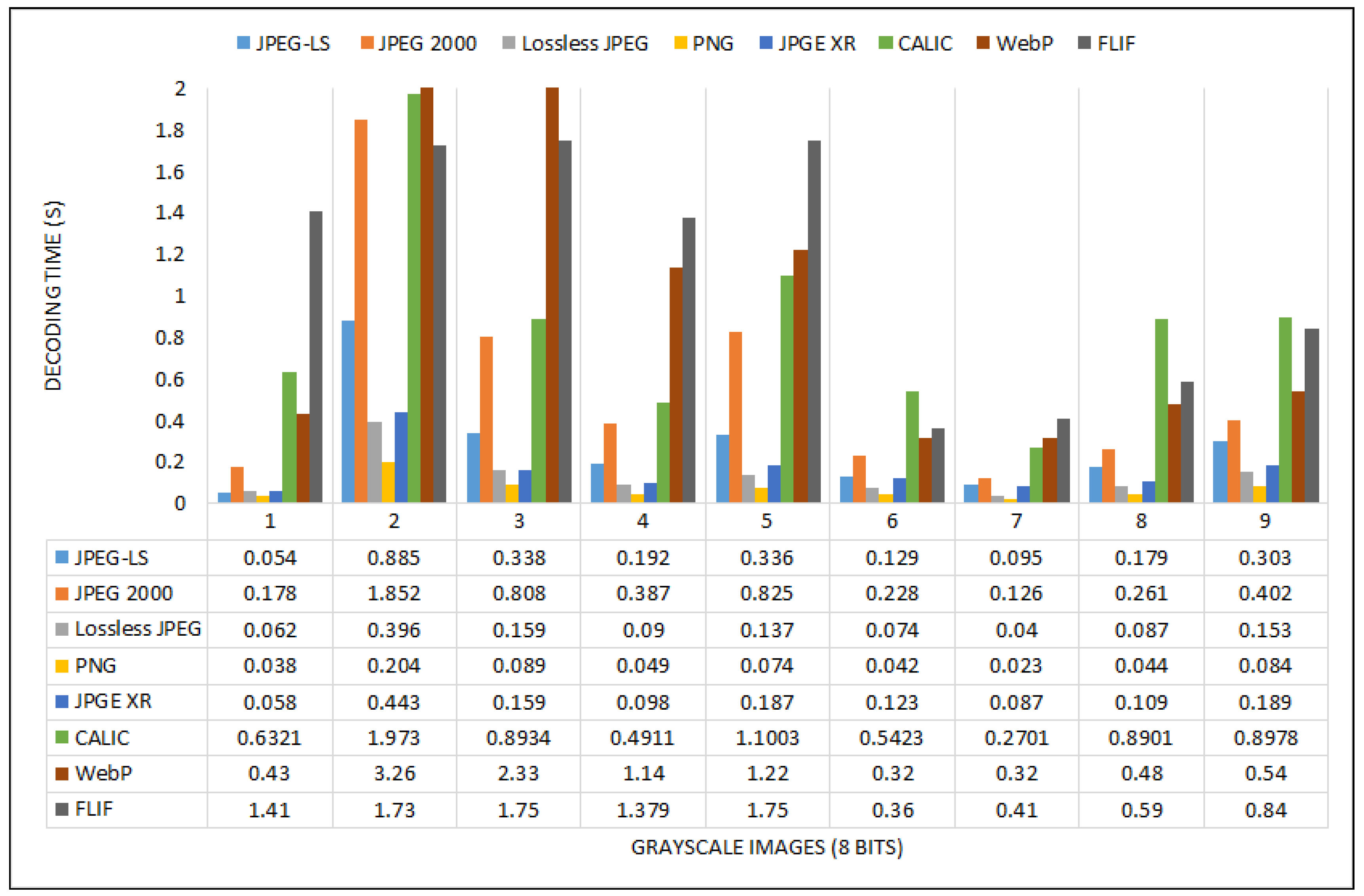
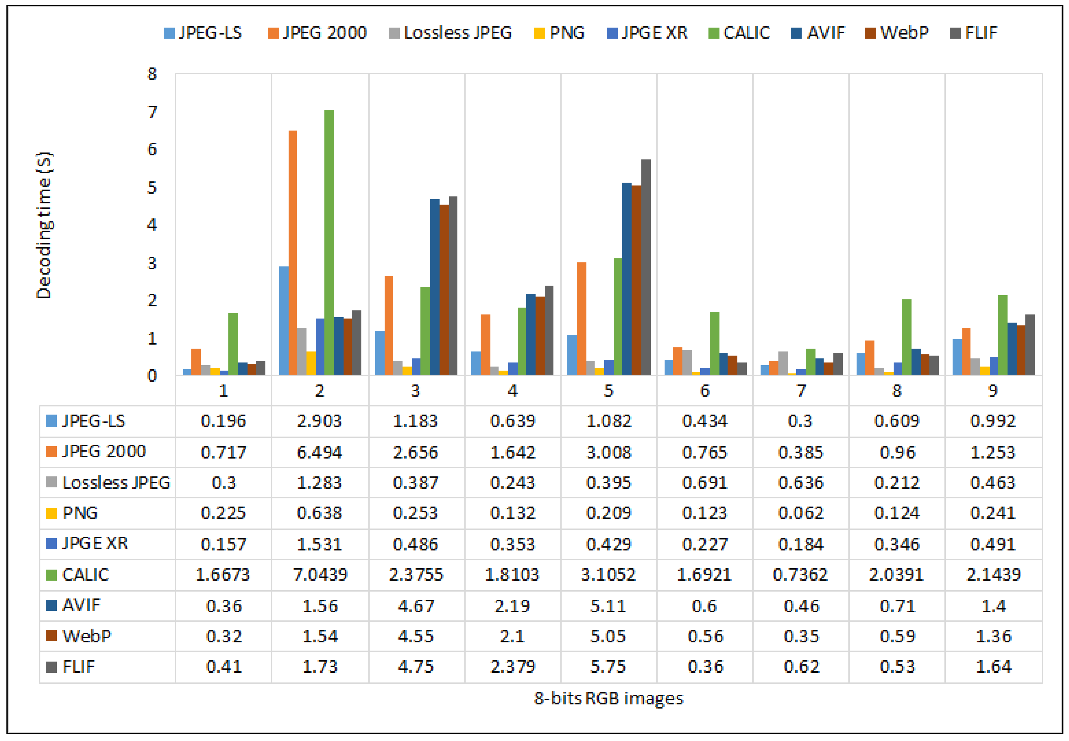
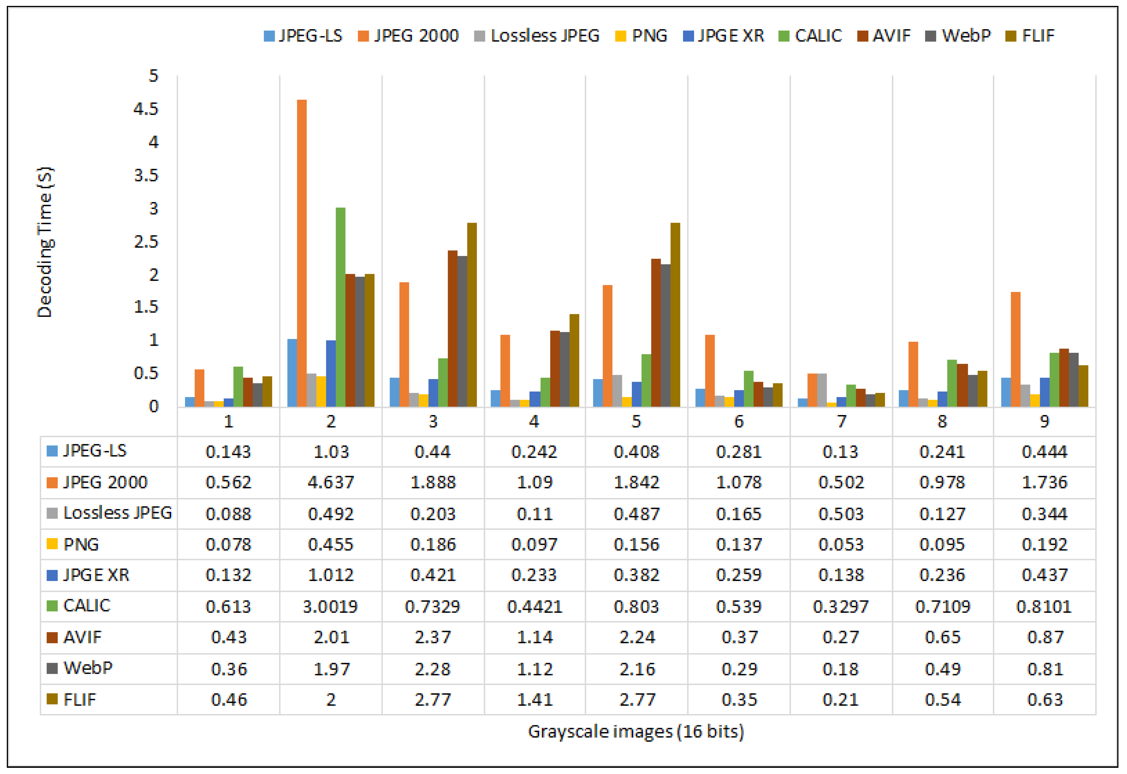
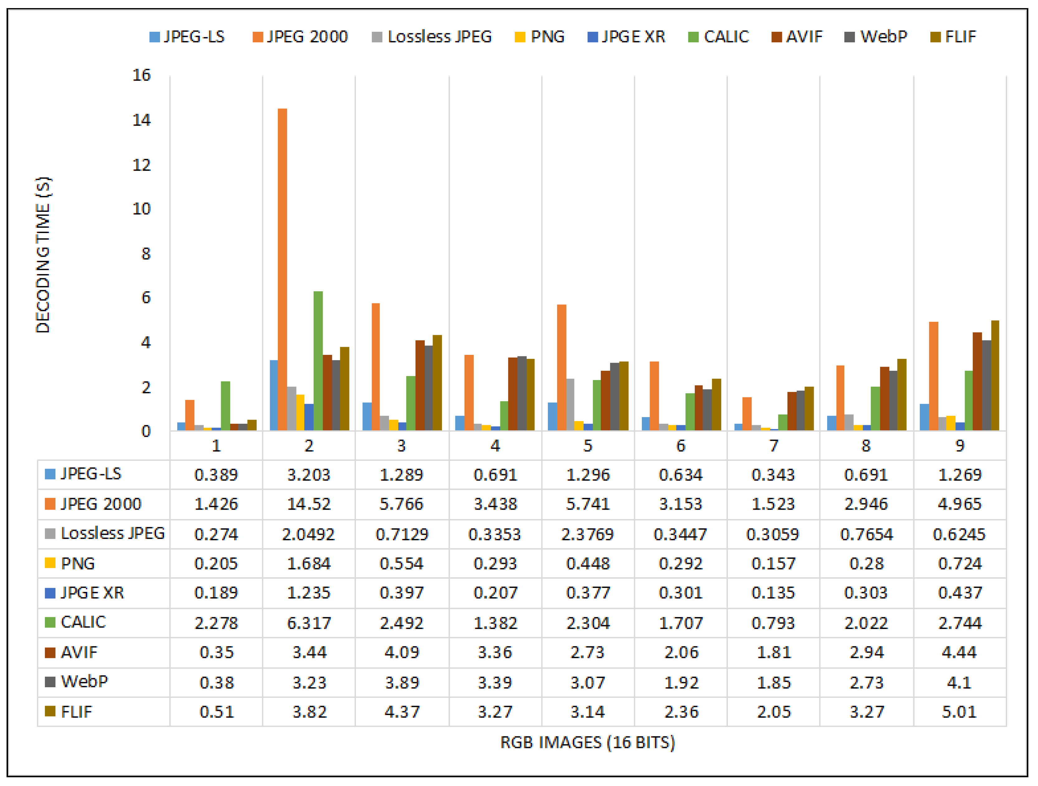
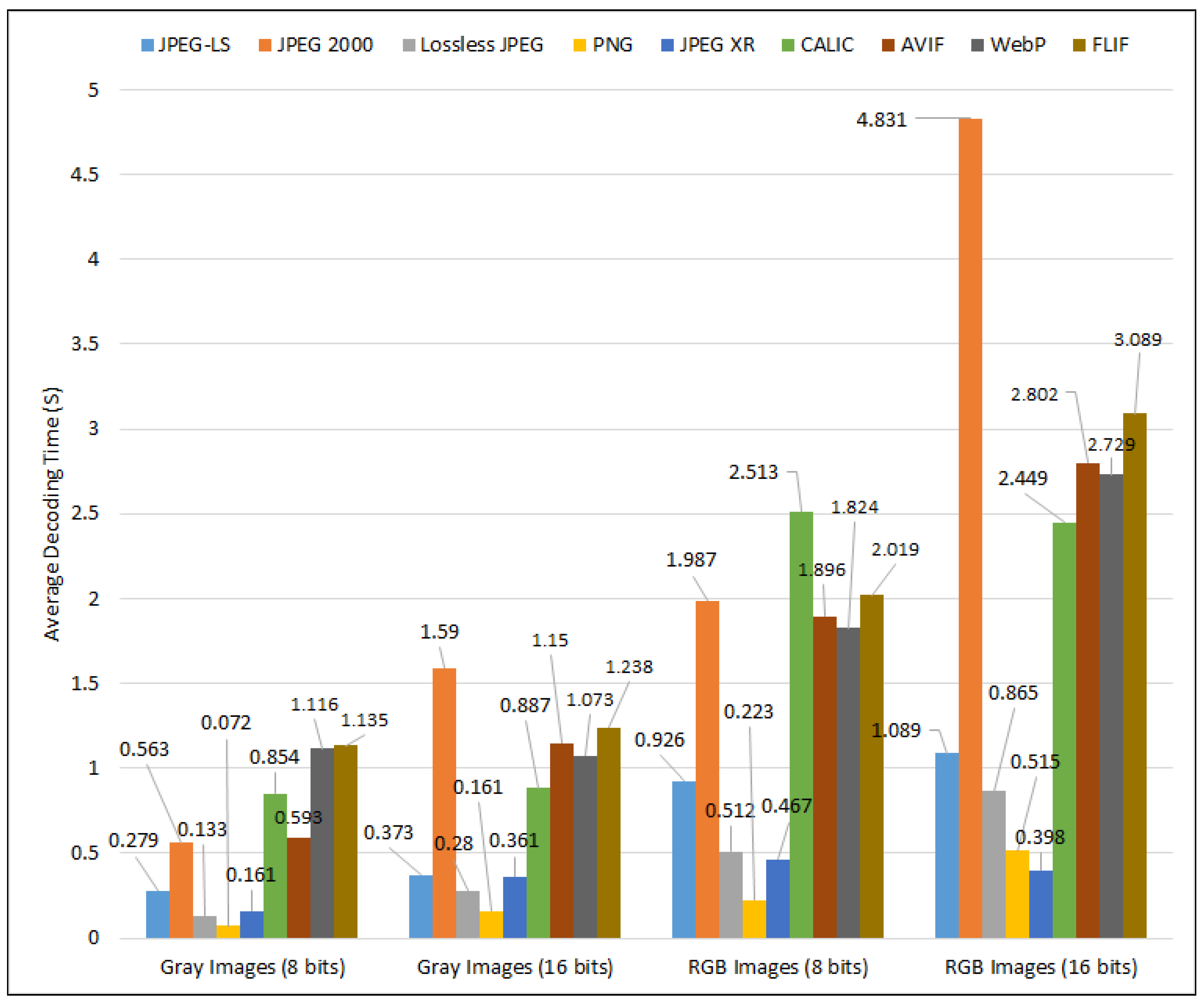
How good is each algorithm in terms of the DT for 8-bit and 16-bit greyscale and RGB images?
RI4:
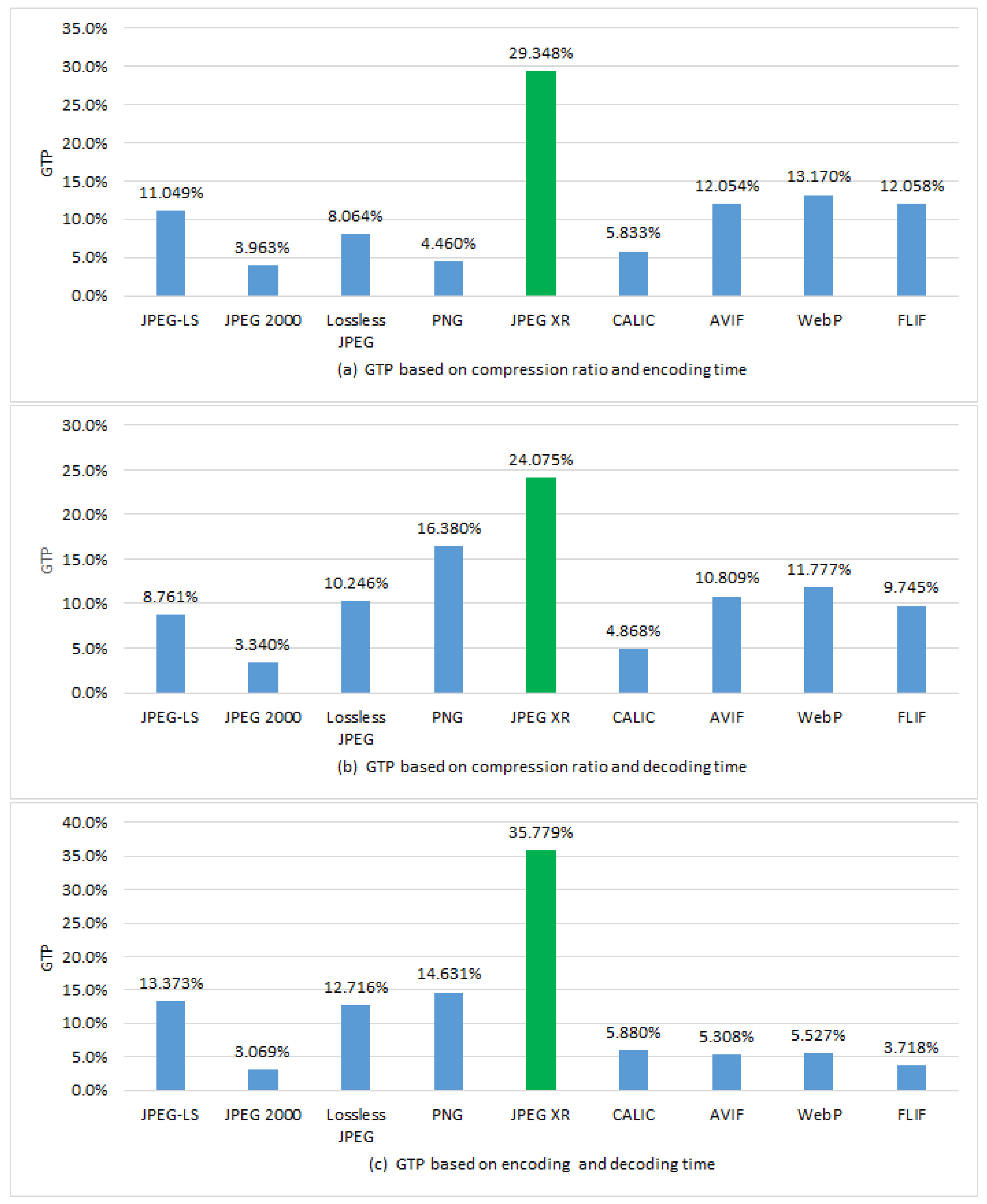
How good is each algorithm in terms of the CR and ET for 8-bit and 16-bit greyscale and RGB images?
RI5:
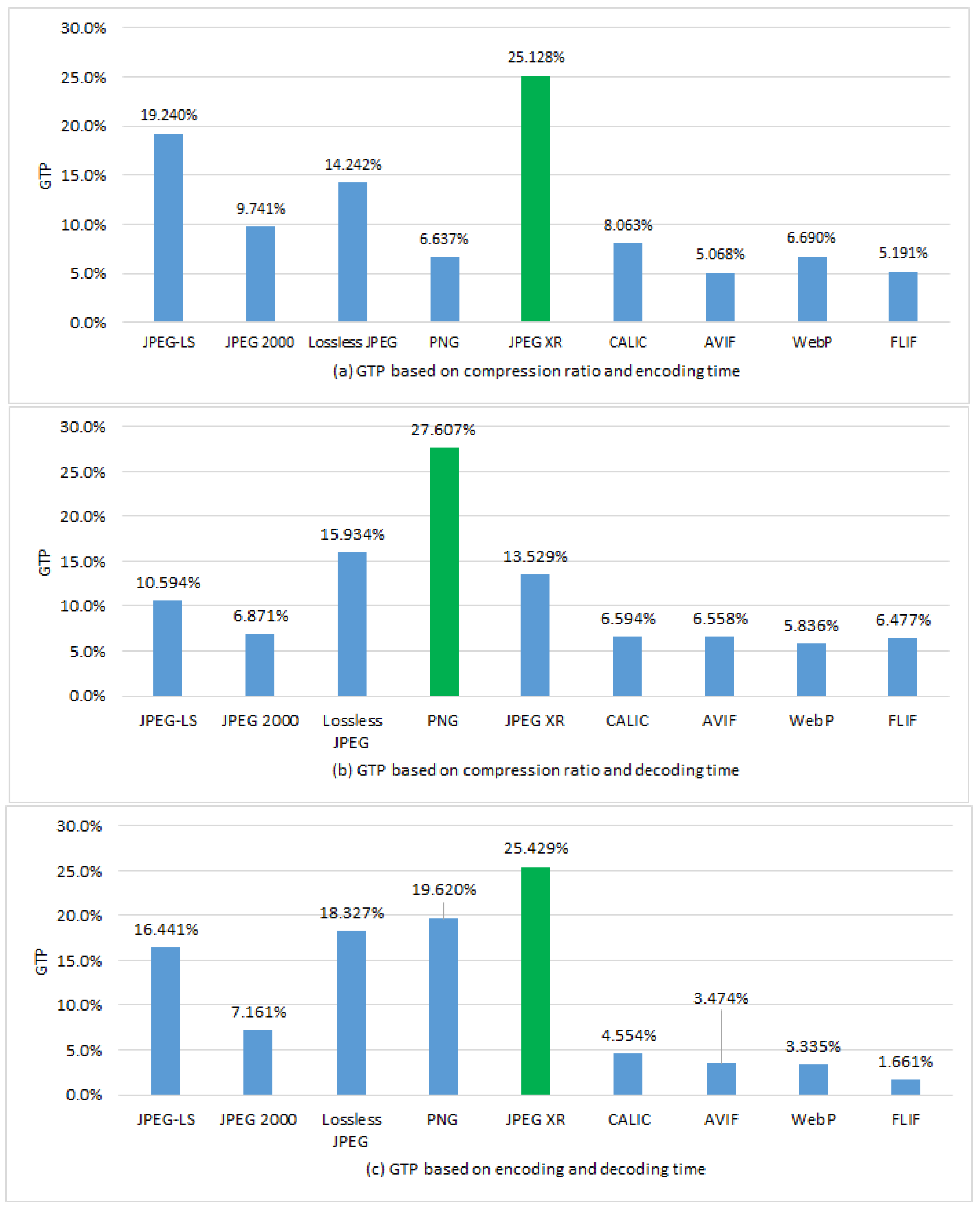
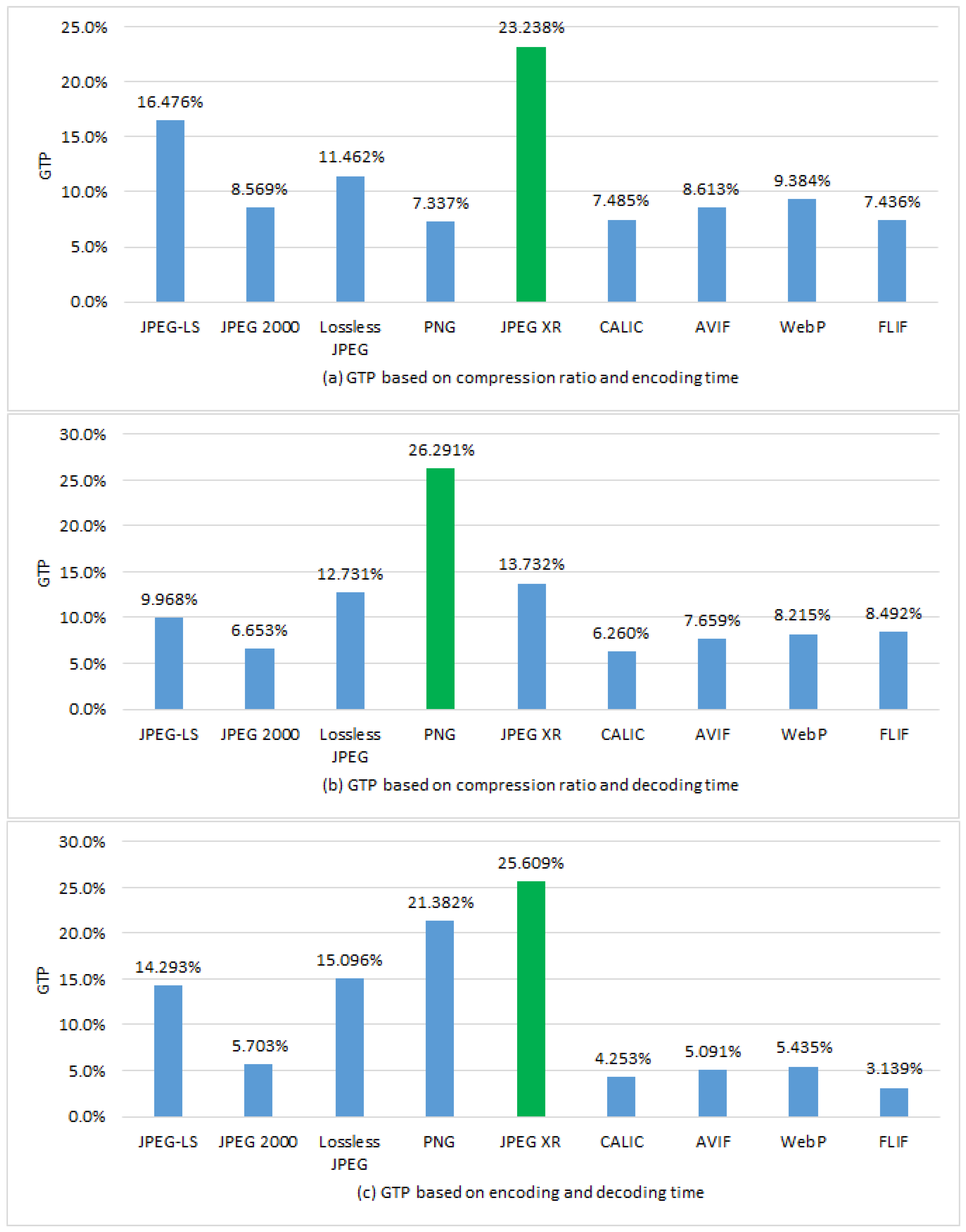
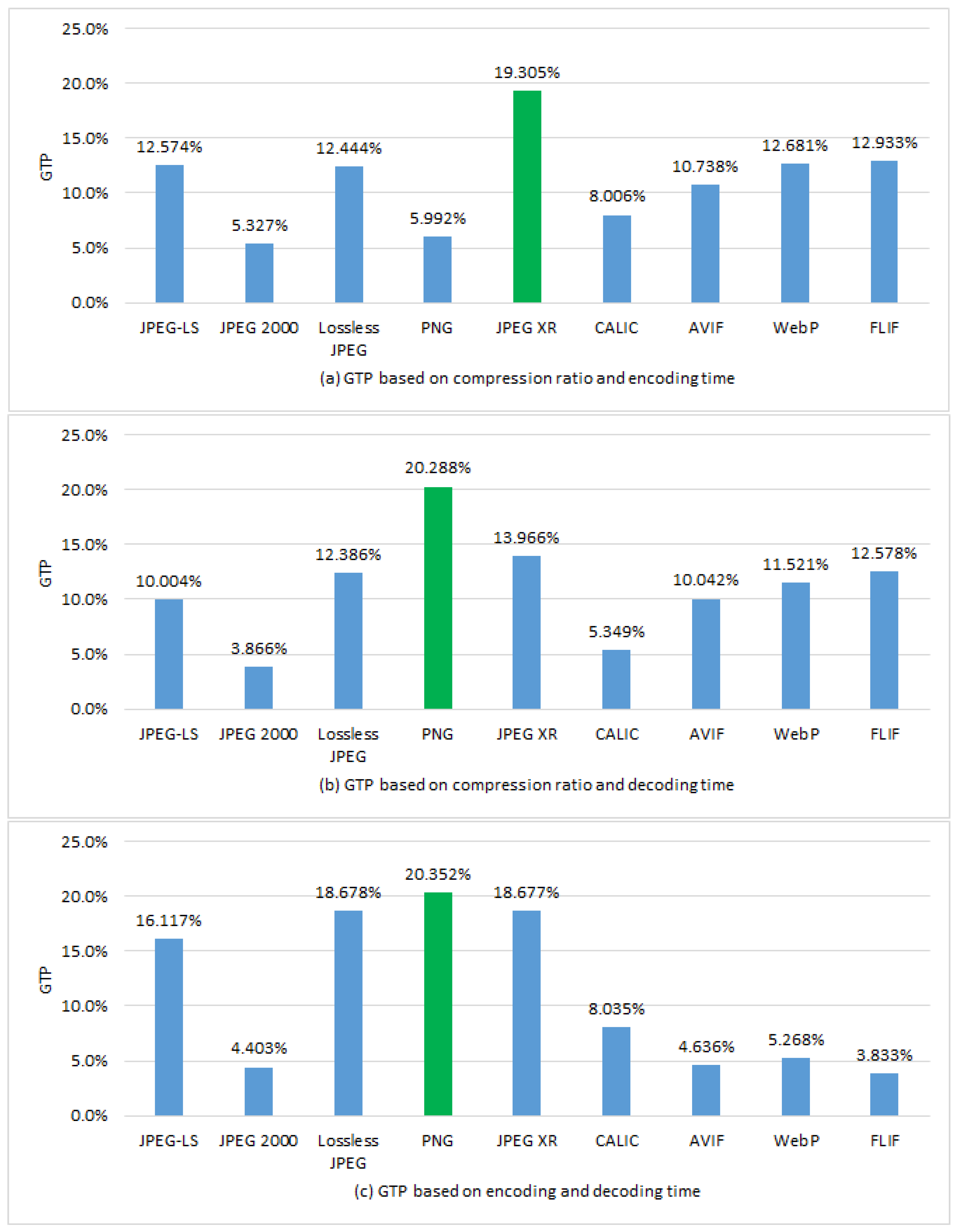
How good is each algorithm in terms of the CR and DT for 8-bit and 16-bit greyscale and RGB images?
RI6:
How good is each algorithm in terms of the ET and DT for 8-bit and 16-bit greyscale and RGB images?
RI7:
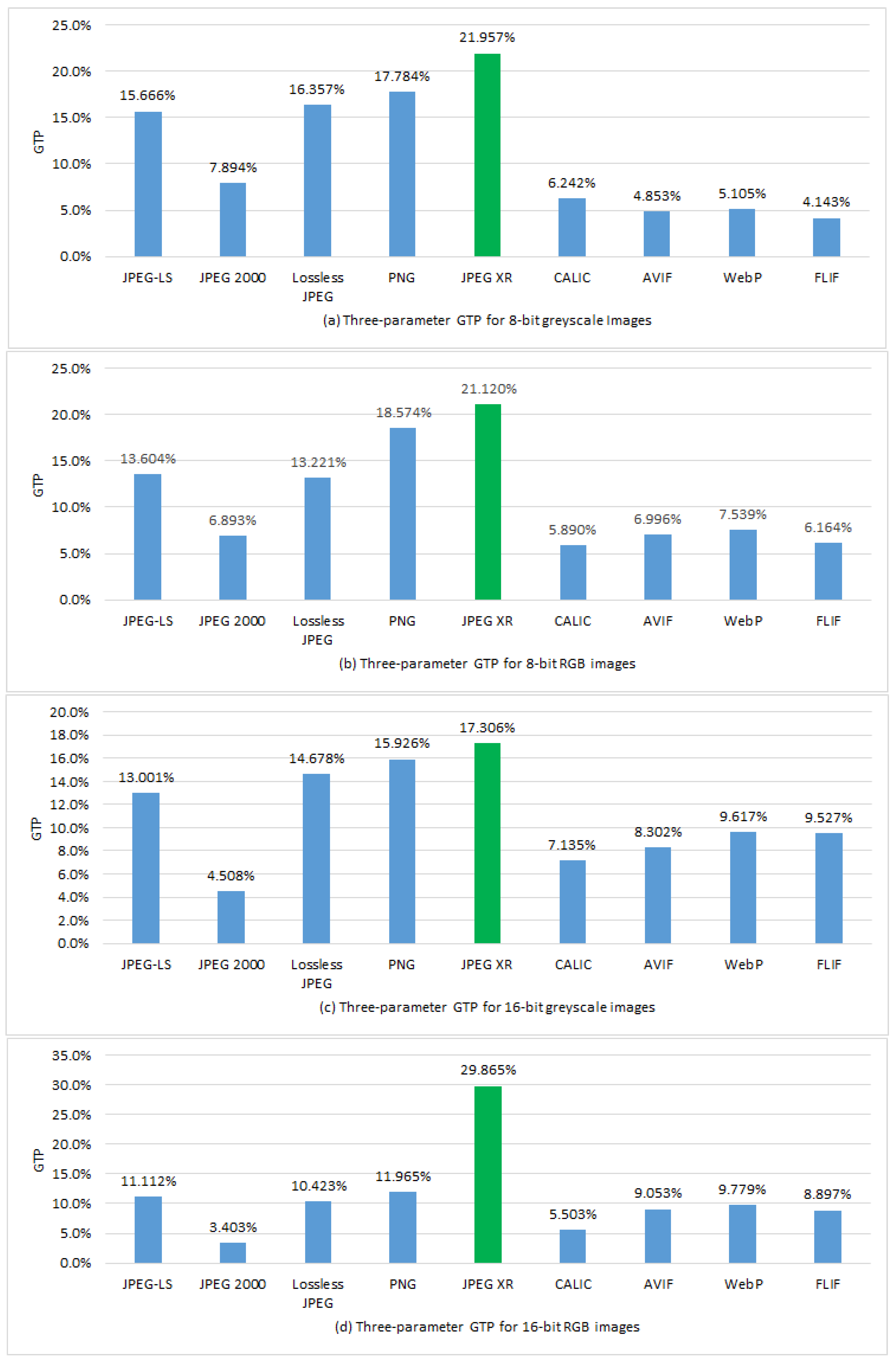
How good is each algorithm when all parameters are equally important for 8-bit and 16-bit greyscale and RGB images?
RI8:
Which algorithms should be used for each kind of image?
The remainder of this article is structured, as follows. In Section 2, we give a brief introduction to the four types of image. In Section 3, we briefly discuss why compression is important, how images are compressed, the kind of changes that occur in data during compression, and the types of data that are targeted during compression. The measurement parameters that are used to evaluate a lossless image compression algorithm are discussed in Section 4. In Section 5, we give a brief introduction to the advanced lossless image compression algorithms. Based on the usual parameters that were used to evaluate a lossless image compression technique and our developed technique, a detailed analysis of the experimental outcomes obtained using these algorithms is provided in Section 6. We conclude the paper in Section 7.

2. Background

A visual representation of an object is called an image, and a digital image can be defined as a two-dimensional matrix of discrete values. When the colour at each position in an image is represented as a single tone, this is referred to as a continuous tone image. The quantised values of a continuous tone image at discrete locations are called the grey levels or the intensity [18], and the pixel brightness of a digital image is indicated by its corresponding grey level. Figure 1 shows the steps that are used to transform a continuous tone image to its digital form.
The bit depth indicates the number of bits used to represent a pixel, where a higher bit depth represents more colours, thus increasing the file size of an image [19]. A greyscale image is a matrix of A × B pixels, and 8-bit and 16-bit greyscale images contain 2 8 = 256 and 2 16 = 65,536 different colours, respectively, where the ranges of colour values are from 0–255 and 0–65,535. Figure 2 and Figure 3 show examples of 8-bit and 16-bit greyscale images, respectively.
A particular way of representing colours is called the colour space, and a colour image is a linear combination of these colours. There are many colour spaces, but the most popular are RGB, hue, saturation, value (HSV), and cyan, magenta, yellow, and key (black) (CMYK). RGB contains the three primary colours of red, green, and blue, and it is used by computer monitors. HSV and CMYK are often used by artists and in the printing industry, respectively [18]. A colour image carries three colours per pixel; for example, because an RGB image uses red, green, and blue, each pixel of an 8-bit RGB image has a precision of 24 bits, and the image can represent 2 24 = 16,777,216 different shades. For a 16-bit RGB image, each pixel has a precision of 48 bits, allowing for 2 48 = 281,474,976,710,656 different shades. Figure 4 and Figure 5 show typical examples of 8-bit and 16-bit RGB images, respectively. The ranges of colour values for 8-bit and 16-bit images are 0–255 and 0–65,535, respectively.
For an uncompressed image (X), the memory that is required to store the image is calculated using Equation (1), where the dimensions of the image are A × B, the bit depth is N, and required storage is S.
S = A B N 2 13 K B

3. Data Compression

Data compression is a significant issue and a subject of intense research in the field of multimedia processing. We give a real example below to allow for a better understanding of the importance of data compression. Nowadays, digital cinema and high-definition television (HDTV) use a 4K system, with approximately 4096 × 2160 pixels per frame [20]. However, the newly developed Super Hi-Vision (SHV) format uses 7680 × 4320 pixels per frame, with a frame rate of 60 frames per second [21]. Suppose that we have a three-hour colour video file that is based on SHV video technology, where each pixel has a precision of 48 bits. The size of the video file will then be ( 7680 × 4320 × 48 × 60 × 3 × 60 × 60 ) bits, or approximately 120,135.498 GB. According to the report in [22], 500 GB to 1 TB is appropriate for storing movies for non-professional users. Seagate, which is an American data storage company, has published quarterly statistics since 2015 on the average capacity of Seagate hard disk drives (HDDs) worldwide. In the third quarter of 2020, this capacity was 4.1 TB [23]. Can we imagine what would have happened? We could not even store a three-hour color SHV video file on our local computer. Compression is another important issue for data transmission over the internet. Although there are many forms of media that can be used for transmission, fibre optic cables have the highest transmission speed [24], and can transfer up to 10 Gbps [25]. If this video file is transferred at the highest speed available over fibre optic media without compression, approximately 26.697 h would be required, without considering latency. Latency is the amount of time that is required to transfer data from the original source to the destination [26]. In view of the above problems, current technology is entirely inadequate, and data compression is the only effective solution.
An image is a combination of information and redundant data. How much information an image contains is one of the most important issues in image compression. If an image contains a number of unique symbols SL, and P(k) is the probability of the kth symbol, the average information content (AIC) that an image may contain, which is also known as entropy, is calculated using Equation (2). Image compression is achieved through a reduction in redundant data.
A I C = k = 1 S L l o g ( P ( k ) ) P ( k )
Suppose that two datasets A and B point to the same image or information. Equation (3) can then be used in order to define the relative data redundancy ( R d r ) of set A, where the CR is calculated using Equation (4).
R d r = 1 1 C R
C R = A B
Three results can be deduced from Equations (3) and (4).
  • When A = B, CR = 1, R d r = 0 , there is no redundancy, and, hence, no compression.
  • When BA, CR → infinite, R d r 1 , dataset A contains the highest redundancy and the greatest compression is achieved.
  • When BA, CR → 0, R d r i n f i n i t e , dataset B contains large memory than the original (A).
In digital image compression, there are three types of data redundancy: coding, inter-pixel, and psycho-visual redundancy [27,28]. Suppose that we have the image that is shown in Figure 6 with the corresponding grey levels.
The 10 × 10 image shown in Figure 6 contains nine different values (S) (118, 119, 120, 139, 140, 141, 169, 170, 171), and for a fixed code length, each value can be coded as an 8-bit code-word, since the maximum value (171) requires a minimum of 8 bits to code. Consequently, 800 bits are required to store the image. In contrast, a variable code length is based on probability, where codes of shorter length are assigned to values with higher probability. The probability of the kth values is calculated while using Equation (5), where N is the total number of values in an image. If L k represents the length of the code-word for the values S k , then the length of the average code-word can be calculated using Equation (6), where SL is the total number of different values. Table 1 shows the variable length coding for the image shown in Figure 6.
P ( k ) = S k N
L a v g = k = 1 S L L k P ( k )
From Table 1, we obtain approximate values of CR = 2.581 and R d r = 0.613 , and the compressed image takes 300 bits rather than 800 bits. These results show that the original image contains redundant code, and that the variable length coding has removed this redundancy [29,30].
Interpixel redundancy can be classified as spatial, spectral, and temporal redundancy. In spatial redundancy, there are correlations between neighbouring pixel values, whereas, in spectral redundancy, there are correlations between different spectral bands. In temporal redundancy, there are correlations between the adjacent frames of a video. Interpixel redundancy can be removed using run-length coding, the differences between adjacent pixels, predicting a pixel using various methods, thresholding, or various types of transformation techniques, such as discrete Fourier transform (DFT) [31].
To remove interpixel redundancy from the image presented in Figure 7 using run-length coding, we code the image, as follows: (120,1) (119,1) (118,8) (120,1) (119,8) (118,1) (120,9) (119,1) (120,1) (119,6) (118,3) (141,1) (140,8) (139,1) (141,6) (140,4) (141,5) (140,5) (171,1) (170,2) (169,7) (171,2) (170,4) (169,4) (171,7) (170,3), requiring 312 bits. Twelve bits are required to code each pair, and an 8-bit code word is used for the grey level, since the maximum gray level is 171. A 4-bit code word is used for the length of the grey level, since the maximum value for the length of the gray level is nine.
The main purpose of using prediction or transformation techniques can be described, as follows. To create a narrow histogram, a prediction or various other types of transformation techniques can be applied to provide a small value for the entropy. For example, we apply the very simple predictor that is given below to the image shown in Figure 6, where A represents the predicted pixels. Figure 7a shows the histogram of the original image, and Figure 7b shows the histogram obtained after applying the predictor that is shown in Equation (7).
A ( p , q ) = A ( p , q 1 ) A ( p , q )
Figure 7 shows that the histogram of the original image contains nine different values, of which eight have approximately the same frequency, and the highest frequency is 17. After applying the predictor, the histogram only contains five values, of which only two (0 and 1) contain 90% of the data, thus giving a better compression ratio. The interpixel redundancy of an image can be removed using one or more techniques in combination. For example, after applying the predictor to the original image presented in Figure 6, we can apply both run-length and Huffman coding, with the result that only 189 bits are required to store the image rather than 800 bits.
The construction of an image compression technique is highly application-specific. Figure 8 shows a general block diagram of lossless image compression and decompression.
The mapping that is shown in Figure 8 is used to convert an image into a non-visual form to decrease the interpixel redundancy. Run-length coding, various transformation techniques, and prediction techniques are typically applied at this stage. At the symbol encoding stage, Huffman, arithmetic, and other coding methods are often used to reduce the coding redundancy. The image data are highly correlated, and the mapping process is a very important way of decorrelating the data and eliminating redundant data. A better mapping process can eliminate more redundant data and give better compression. The first and most important problem in image compression is to develop or choose an optimal mapping process, while the second is to choose an optimal entropy coding technique to reduce coding redundancy [32]. In channel encoding, Hamming coding is applied to increase noise immunity, whereas, in decoding, the inverse procedures are applied to provide a lossless decompressed image. Quantisation, which is an irreversible process, removes irrelevant information by reducing the number of grey levels, and it is applied between the mapping and symbol encoding stages in lossy image compression [33,34,35,36,37,38].

4. Measurement Standards

Measurement standards offer ways of determining the efficiency of an algorithm. The four measurement standards (compression ratios, encoding time, decoding time, and bits per pixel) are used to evaluate a lossless image compression algorithm.
The CR is the ratio between the size of an uncompressed image and its compressed version. Entropy is generally estimated as the average code length of a pixel in an image; however, in reality, this estimate is overoptimistic due to statistical interdependencies among pixels. For example, Table 1 shows that the CR is 2.581, but the estimated entropy for the same data is 3.02. Hence, the entropy-based compression ratio is 2.649. Equation (4) is used to calculate the CR to solve this issue. The bpp [39] is the number of bits used to represent a pixel, i.e. the inverse of the CR, as shown in Equation (8). The ET and DT are the times that are required by an algorithm to encode and decode an image, respectively.
b p p = B A

5. State-of-the-Art Lossless Image Compression Techniques

The algorithms used for lossless image compression can be classified into four categories: entropy coding (Huffman and arithmetic coding), predictive coding (lossless JPEG, JPEG-LS, PNG, CALIC), transform coding (JPEG 2000, JPEG XR), and dictionary-based coding (LZW). All of the predictive and transform-based image compression techniques use an entropy coding strategy or Golomb coding as part of their compression procedure.

5.1. Lossless JPEG and JPEG-LS

The Joint Photographic Experts Group (JPEG) format is a DCT-based lossy image compression technique, whereas lossless JPEG is predictive. Lossless JPEG uses the 2D differential pulse code modulation (DPCM) scheme [40], and it predicts a value ( P ¯ ) for the current pixel ( P ) that is based on up to three neighbouring pixels (A, B, D). Table 2 shows the causal template used to predict a value. If two pixels (B, D) from Table 2 are considered in this prediction, then the predicted value ( P ¯ ) and prediction error ( P E ¯ ) are calculated while using Equations (9) and (10), respectively.
P ¯ = D + B 2
P E ¯ = P P ¯
Consequently, the prediction errors remain close to zero, and very large positive or negative errors are not commonly seen. Therefore, the error distribution looks almost like a Gaussian normal distribution. Finally, Huffman or arithmetic coding is used to code the prediction errors. Table 3 shows the predictor that is used in the lossless JPEG format, based on three neighbouring pixels (A, B, D). In lossy image compression, three types of degradation typically occur and should be taken into account when designing a DPCM quantiser: granularity, slope overload, and edge-busyness [41]. DPCM is most sensitive to channel noise.
A real image usually has a nonlinear structure, and the DPCM uses a linear predictor, This is why problems can occur. This gave rise to the need to develop a perfect nonlinear predictor. The median edge detector (MED) is one of the most widely used nonlinear predictors, which is used by JPEG-LS to address these drawbacks.
JPEG-LS was designed based on LOCO-I (Low Complexity Lossless Compression for Images) [42,43], and a standard was eventually introduced in 1999 after a great deal of development [44,45,46,47]. JPEG-LS improves the context modelling and encoding stages by applying the same concept as lossless JPEG. Although the discovery of arithmetic codes [48,49] conceptually separates the stages, the separation process becomes less clean under low-complexity coding constraints, due to the use of an arithmetic coder [50]. In context modelling, the number of parameters is an important issue, and it must be reduced to avoid context dilution. The number of parameters depends entirely on the number of context. A two-sided geometric distribution (TSGD) model is assumed for the prediction residuals to reduce the number of parameters. The selection of a TSGD model is a significant issue in a low-complexity framework, since a better model only needs very simple coding. Merhav et al. [51] showed that adaptive symbols can be used in a scheme, such as Golomb coding, rather than more complex arithmetic coding, since the structure of Golomb codes provides a simple calculation without requiring the storage of code tables. Hence, JPEG-LS uses Golomb codes at this stage. Lossless JPEG cannot provide an optimal CR, because it cannot de-correlate by first order entropy of their prediction residuals. In contrast, JPEG-LS can achieve good decorrelation and provide better compression performance [42,43]. Figure 9 shows a general block diagram for JPEG-LS.
The prediction or decorrelation process of JPEG-LS is completely different from that in lossless JPEG. The LOCO-I or MED predictor used by JPEG-LS [52] predicts a value ( P ¯ ) according to Equation (11), as shown in Table 2.
P ¯ = m i n ( D , B ) , if C m a x ( D , B ) m a x ( D , B ) , if C m i n ( D , B ) D + B A , otherwise .

5.2. Portable Network Graphics

Portable Network Graphics (PNG) [53,54,55], a lossless still image compression scheme, is an improved and patent-free replacement of the Graphics Interchange Format (GIF). It is also a technique that uses prediction and entropy coding. The deflate algorithm, which is a combination of LZ77 and Huffman coding, is used as the entropy coding technique. PNG uses five types of filter for prediction [56], as shown in Table 4 (based on Table 2).

5.3. Context-Based, Adaptive, Lossless Image Codec
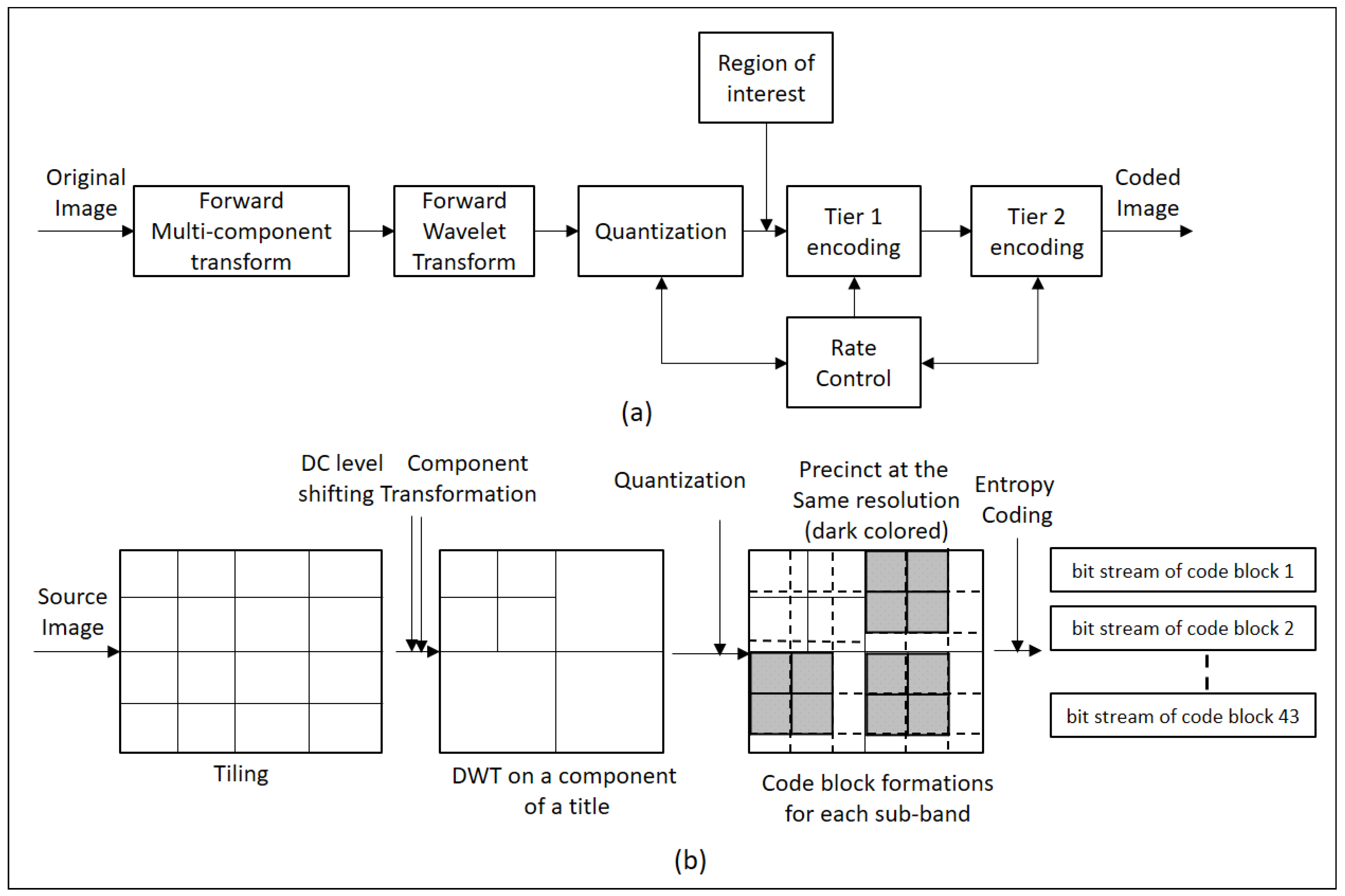
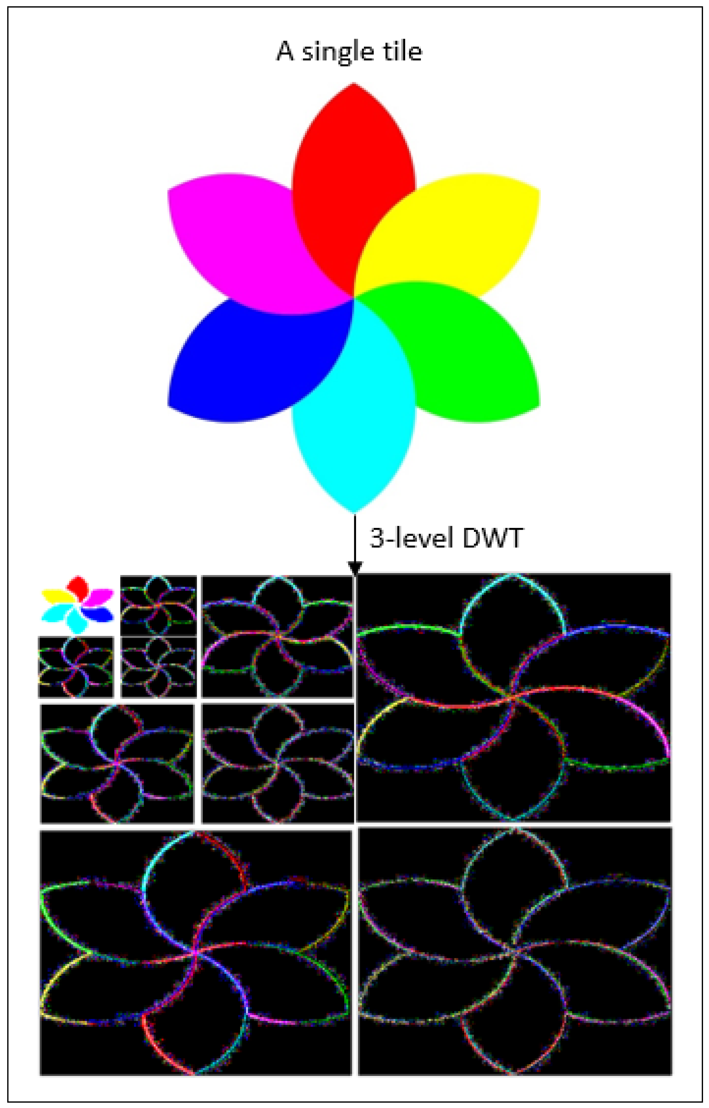
Context-based, adaptive, lossless image codec (CALIC) is a lossless image compression technique that uses a more complex predictor (gradient-adjusted predictor, GAP) than lossless JPEG, PNG, and JPEG-LS. GAP provides better modelling than MED by classifying the edges of an image as either strong, normal, or weak. Although CALIC provides more compression than JPEG-LS and better modelling, it is computationally expensive. Wu [57] used the local horizontal (Gh).and vertical (Gv) image gradients (Equations (12) and (13)) to predict a value ( P ¯ ) (Equation (14)) for the current pixel (P) using Equation (15), as shown in Table 2. At the coding stage, CALIC uses either Huffman coding or arithmetic coding; the latter provides more compression, but it takes more time for encoding and decoding, since arithmetic coding is more complex. The encoding and decoding methods in CALIC follow a raster scan order, with a single pass of an image. There are two modes of operation, binary and continuous tone. If the current locality of an original image has a maximum of two distinct intensity values, binary mode is used; otherwise, continuous tone mode is used. The continuous tone approach has four components: prediction, context selection and quantisation, context modelling of prediction errors, and entropy coding of the prediction errors. The mode is selected automatically, and no additional information is required [58].
G h = | D K | + | B A | + | C B |
G v = | D A | + | B F | + | C G |
P ¯ = D , if ( G v G h > 80 ) ; Sharp   horizontal   edge M + P 2 , if ( G v G h > 32 ) ; Horizontal   edge 3 × M + P 4 , if ( G v G h > 8 ) ; Weak   horizontal   edge B , if ( G v G h < 80 ) ; Sharp   vertical   edge M + B 2 , if ( G v G h < 32 ) ; Vertical   edge 3 × M + B 4 , if ( G v G h < 8 ) ; Weak   vertical   edge
M = D + B 2 + C A 4

5.4. JPEG 2000

JPEG 2000 is an extension complement of the JPEG standard [40], and it is a wavelet-based still image compression technique [59,60,61,62] with certain new functionalities. It provides better compression than JPEG [60]. The development of JPEG 2000 began in 1997, and became an international standard [59] in 2000. It can be used in lossless or lossy compression within a single architecture. Most image or video compression standards divide an image or a video frame into square blocks, to be processed independently. For example, JPEG uses the Discrete Cosine Transform (DCT) in order to split an image into a set of 8 × 8 square blocks for transformation. As a result of this processing, extraneous blocking artefacts arise during the quantisation of the DCT coefficients at high CR [7], producing visually perceptible faults in the image [61,62,63,64]. In contrast, JPEG 2000 transforms an image as a whole while using a discrete wavelet transformation (DWT), and this addresses the issue. One of the most significant advantages of using JPEG 2000 is that different parts of the same image can be saved with different levels of quality if necessary [65]. Another advantage of using DWT is that it transforms an image into a set of wavelets, which are easier to store than pixel blocks [66,67,68]. JPEG 2000 is also scalable, which means that a code stream can be truncated at any point. In this case, the image can be constructed, but the resolution may be poor if many bits are omitted. JPEG 2000 has two major limitations: it produces ringing artifacts near the edges of an image, and is computationally more expensive [69,70]. Figure 10 shows a general block diagram for the JPEG 2000 encoding technique.
Initially, an image is transformed into the YUV colour space, rather than YCbCr, for lossless JPGE2000 compression, since YCbCr is irreversible and YUV is completely reversible. The transformed image is then split into a set of tiles. Although the tiles may be of any size, all of the tiles in an image are the same size. The main advantage of dividing an image into tiles is that the decoder requires very little memory for image decoding. In this tiling process, the image quality can be decreased for low PSNR, and the same blocking artifacts, like JPEG, can arise when more tiles are created. The LeGall-Tabatabai (LGT) 5/3 wavelet transform is then used to decompose each tile for lossless coding [71,72], while the CDF 9/7 wavelet transform is used for lossy compression [72].
Quantisation is carried out in lossy compression, but not in lossless compression. The outcome of the transformation process is the sub-band collection and the sub-bands are further split into code blocks, which are then coded while using the embedded block coding with optimal truncation (EBCOT) process, in which the most significant bits are coded first. All of the bit planes of the code blocks are perfectly stored and coded, and a context-driven binary arithmetic coder is applied as an entropy coder independently to each code block. Some bit planes are dropped in lossy compression. While maintaining the same quality, JPEG 2000 provides about 20% more compression than JPEG and it works better for larger images.
After the DWT transformation of each tile, we obtain four parts: the top left image with lower resolution, the top right image with higher vertical resolution, the bottom left image with lower vertical resolution, and the bottom right image with higher resolution in both directions. This decomposition process is known as dyadic [60], and it is illustrated in Figure 11 based on a real image, where the entire image is considered as a single tile.

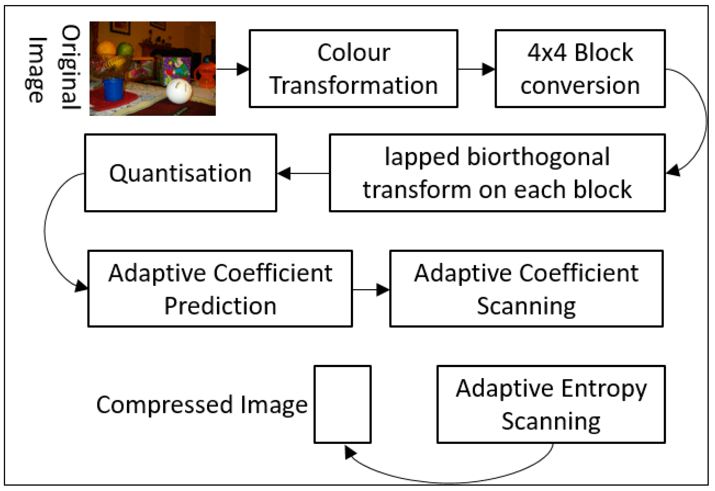
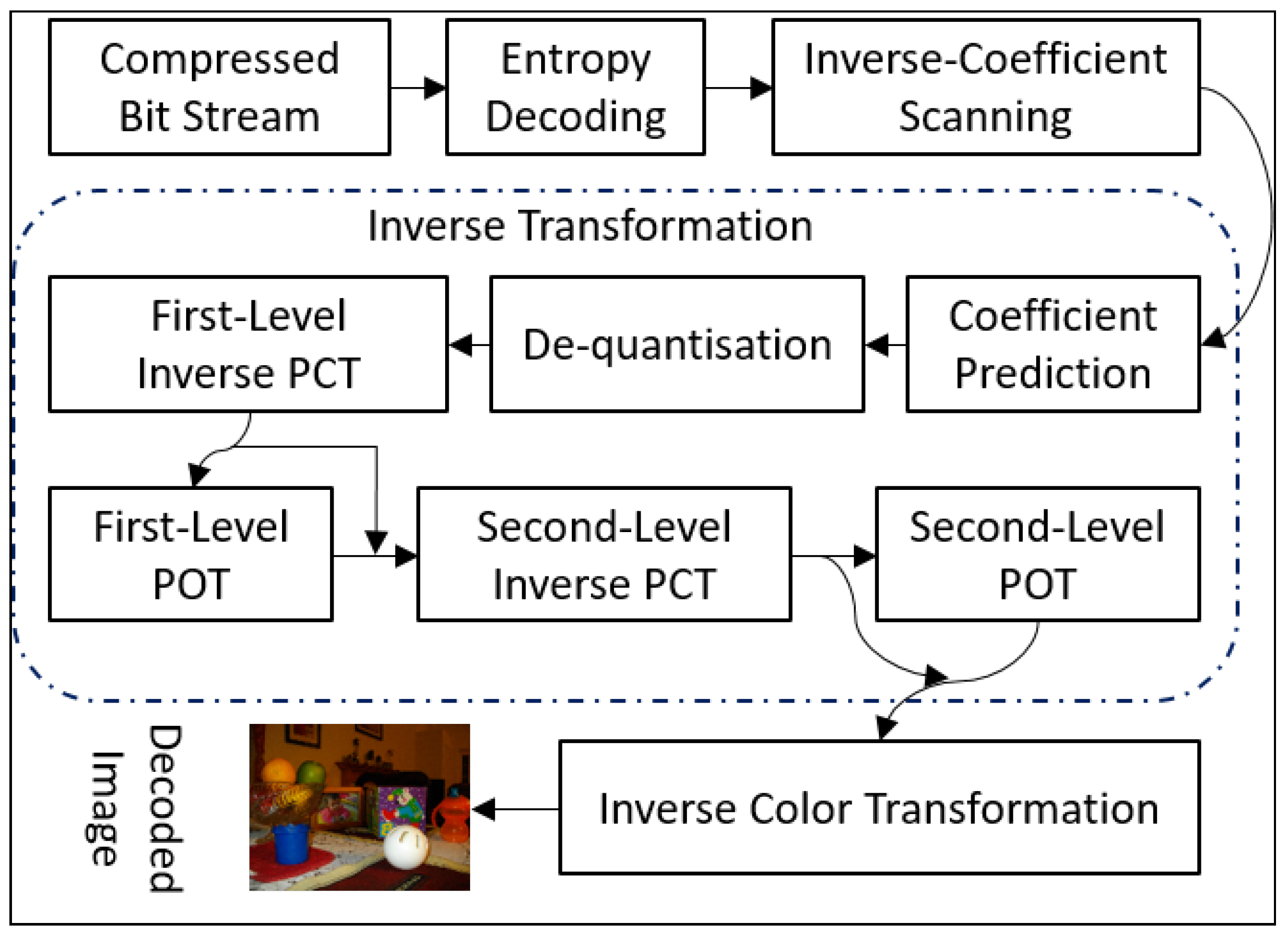
5.5. JPEG XR (JPEG Extended Range)

Like JPEG, JPEG Extended Range (JPEG XR) is a still image compression technique that was developed based on HD photo technology [73,74]. The main aim of the design of JPEG XR was to achieve better compression performance with limited computational resources [75], since many applications require a high number of colours. JPEG XR can represent 2.8 ×   10 14 colours, as compared to only 16,777,216 for JPEG. While JPEG-LS, CALIC, and JPEG 2000 use MED, GAP, and DWT, respectively, for compression, JPEG XR uses a lifting-based reversible hierarchical lapped biorthogonal transform (LBT). The two main advantages of this transformation are that encoding and decoding both require relatively few calculations, and they are completely reversible. Two operations are carried out in this transformation: a photo core transform (PCT), which employs a lifting scheme, and a photo overlap transform (POT) [76]. Similar to DCT, PCT is a 4 × 4 wavelet-like multi-resolution hierarchical transformation within a 16 × 16 macroblock. This transformation improves the image compression performance [76]. POT is performed before PCT to reduce blocking artifacts at low bitrates. Another advantage of using POT is that it reduces the ET and DT at high bitrates [77]. At the quantisation stage, a flexible coefficient quantisation approach that is based on the human visual system is used that is controlled by a quantisation factor (QF), where QF varies, depending on the colour channels, frequency bands, and spatial regions of the image. It should be noted that quantisation is only done for lossy compression. An inter-block coefficient prediction technique is also implemented to remove inter-block redundancy [74]. Finally, JPEG XR uses adaptive Huffman coding as an entropy coding technique. JPEG XR also allows for image tiling in the same way as JPEG 2000, which means that the decoding of each block can be done independently. JPEG XR permits multiple colour conversions, and uses the YCbCr colour space for images with 8 bits per sample and the YCoCg color space for RGB images. It also supports the CMYK colour model [73]. Figure 12 and Figure 13 show general block diagrams for JPEG XR encoding and decoding, respectively.

5.6. AV1 Image File Format (AVIF), WebP and Free Lossless Image Format (FLIF)

In 2010, Google introduced WebP based on VP8 [79]. It is now one of the most successful image formats and it supports both lossless and lossy compression. WebP predicts each block based on three neighbor blocks, and the blocks are predicted in four modes: horizontal, vertical, DC, and TrueMotion [80,81]. Though WebP provides better compression than JPEG and PNG, only some browsers support WebP. Another disadvantage is that lossless WebP does not support progressive decoding [82]. A clear explanation of the encoding procedure of WebP has been given in [83].
AOMedia Video 1 (AV1), which was developed in 2015 for video transmission, is a royalty-free video coding format [84], and AV1 Image File Format (AVIF) is derived from AV1 and it uses the same technique for image compression. It supports both lossless and lossy compression. AV1 uses a block-based frequency transform and incorporates some new features that are based on Google’s VP9 [85]. As a result, the AV1’s encoder gets more alternatives to allow for better adaptation to various kinds of input and outperforms H.264 [86]. The detailed coding procedure of AV1 is given in [87,88]. AVIF and HEIC provide almost similar compression. HEIC is patent-encumbered H.265 format and illegal to use without obtaining patent licenses. On the other hand, AVIF is free to use. There are two biggest problems in AVIF. It is very slow for encoding and decoding an image, and it does not support progressive rendering. AVIF provides many advantages over WebP. For example, it provides a smaller sized image and a more quality image, and it supports multi-channel [89]. A detailed encoding procedure of AV1 is shown in [90].
Free Lossless Image Format (FLIF) is one of the best lossless image formats and it provides better performance than the state-of-the-art techniques in terms of compression ratio. Many image compression techniques (e.g., PNG) support progressive decoding that can show an image without downloading the whole image. In this stage, FLIF is better, as it uses progressive interlacing, which is an improved version of the progressive decoding of PNG. FLIF is developed based on MANIAC (Meta-Adaptive Near-zero Integer Arithmetic Coding), a variant of CABAC (context-adaptive binary arithmetic coding. The detailed coding explanation of FLIF is given in [91,92]. One of the main advantages of FLIF is that it is responsive by design. As a result, users can use it, as per their needs. FLIF provides excellent performances on any kind of image [93]. In [91], Jon et al. show that JPEG and PNG work well on photographs and drawings images, respectively, and there is no single algorithm that works well on all types of images. However, they finally conclude that only FLIF works better on any kinds of image. FLIF has many limitations, such as no browser still supports FLIF [94], and it takes more time for encoding and decoding an image.

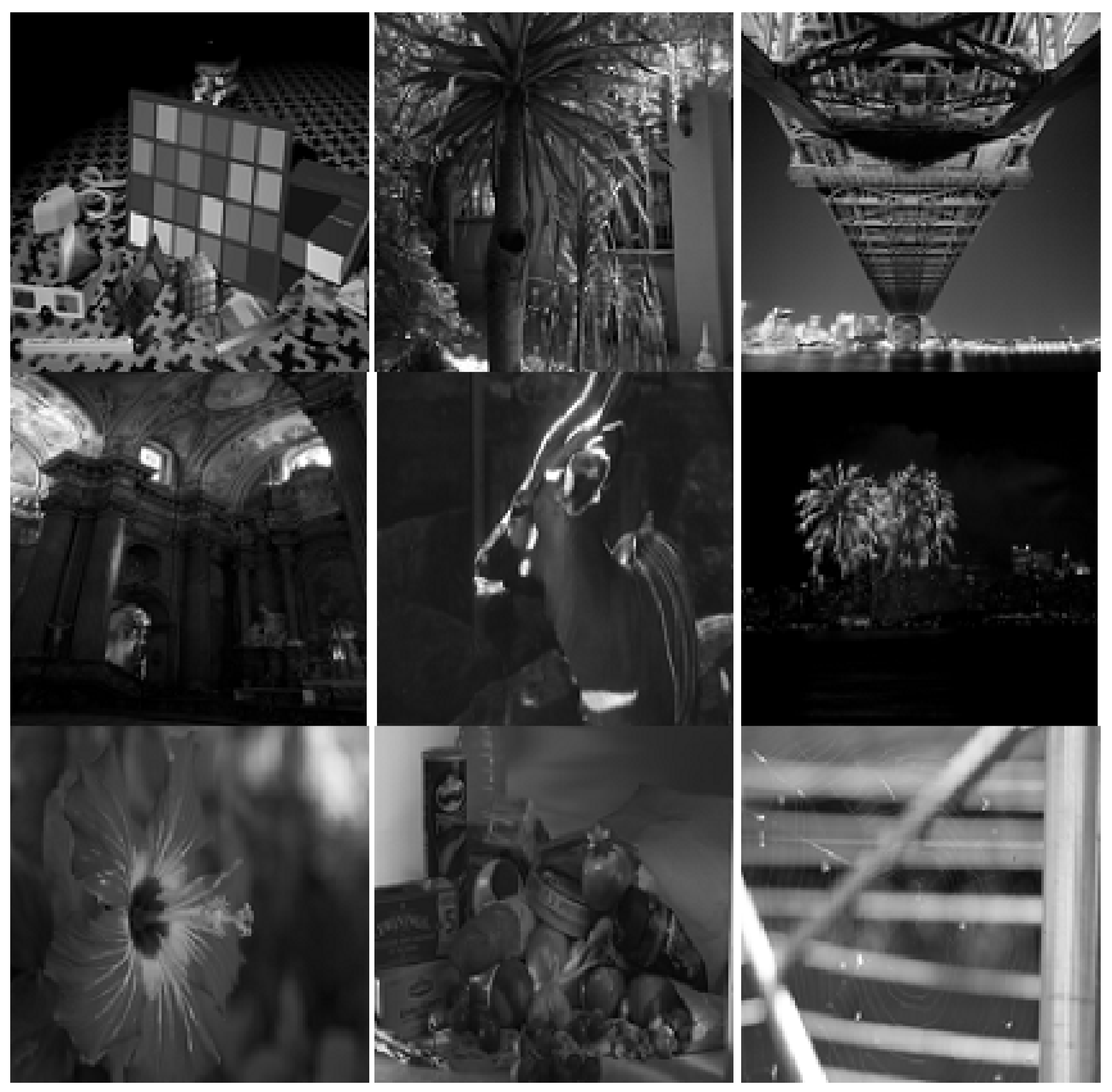
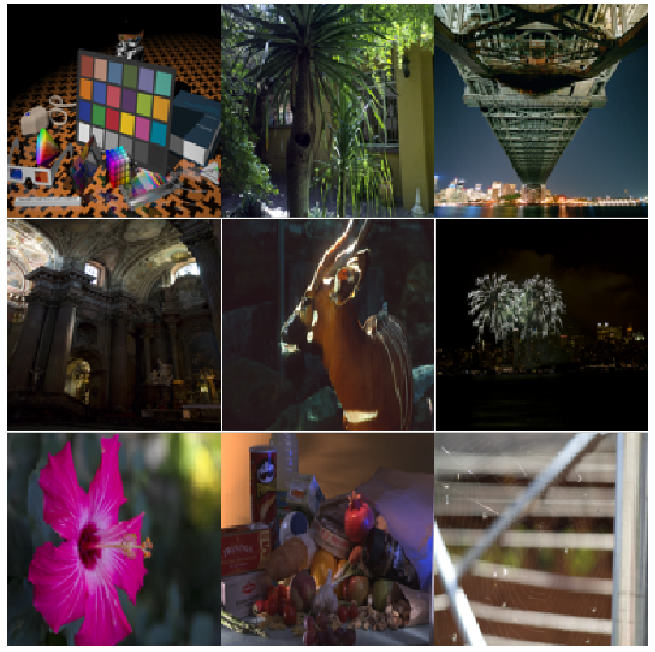
6. Experimental Results and Analysis

The dependence of many applications on multimedia computing is growing rapidly, due to an increase in the use of digital imagery. As a result, the transmission, storage, and effective use of images are becoming important issues. Raw image transmission is very slow, and gives rise to huge storage costs. Digital image compression is a way of converting an image into a format that can be transferred quickly and stored in a comparatively small space. In this paper, we provide a detailed analysis of the state-of-the-art lossless still image compression techniques. As we have seen, most previous survey papers on lossless image compression focus on the CR [3,4,16,78,95,96,97,98]. Although this is an important measurement criterion, the ET and DT are two further important factors for lossless image compression. The key feature of this paper is that we not only carry out a comparison based on CR, but also explore the effectiveness of each algorithm in terms of compressing an image based on several metrics. We use four types of images: 8-bit and 16-bit greyscale and RGB images. We applied state-of-the-art techniques to a total of nine uncompressed images of each type, taken from a database entitled “New Test Images—Image Compression Benchmark” [99].

6.1. Analysis Based on Usual Parameters

In this section, we have analysed based on every single parameter. Figure 14, Figure 15 and Figure 16 show the 8-bit greyscale images and their respective ETs and DTs, and Table 5 shows the CRs of the images. Table 5 shows that FLIF gives the highest CR for the artificial.pgm, big_tree.pgm, bridge.pgm, cathedral.pgm, fireworks.pgm, and spider_web.pgm 8-bit greyscale images. For the rest of the images, AVIF provides the highest CR. JPEG XR gives the lowest CRs (3.196, 3.054, and 2.932) for three images (artificial, fireworks and flower_foveon, respectively), while for the rest of the images, lossless JPEG gives the lowest CR. In terms of the ET, Figure 15 shows that JPEG-LS gives the shortest times (0.046 and 0.115 s) for two images (artificial and fireworks) and JPEG XR gives the shortest times for the remainder of the images. FLIF takes the longest times ( 3.28, 15.52, 6.18, 2.91, 6.19, 2.73, 3.27 and 4.32 s, respectively) for all the images, except flower_foveon.pgm. For this image, AVIF takes the longest time (1.54 s). Figure 16 shows that, at the decoding stage, CALIC takes the longest times (0.542, 0.89, and 0.898 s) for three images (fireworks.pgm, hdr.pgm, and spider_web.pgm, respectively), and WebP takes the longest times (3.26 and 2.33 s) for two images (big_tree.pgm and bridge.pgm, respectively), while FLIF takes the longest times for the rest of the images. On the other hand, PNG takes the shortest times, respectively, for all of the images.
Figure 17 shows examples of 8-bit RGB images. Table 6 and Figure 18 and Figure 19 show the values of CR, ET, and DT for each of the images. From Table 6, it can be seen that FLIF gives the highest CRs (18.446 and 5.742) for two images (artificial.PPM and fireworks.PPM, respectively), and AVIF gives the highest CRs for the rest of the images. JPEG XR gives the lowest CRs (4.316 and 3.121) for two images (artificial and fireworks, respectively) and, for the remaining seven images, lossless JPEG gives the lowest CRs. Figure 18 shows that FLIF requires the longest ETs for all the images. JPEG XR gives the shortest ET for all images, except artificial.pgm, for which JPEG-LS gives the shortest ET (0.16 s). For decoding, CALIC takes the longest time for all images, except for bridge, cathedral, and deer, as shown in Figure 19, and FLIF takes the longest times (4.75, 2.379, and 5.75 s, respectively) for these images. Figure 19 also shows that JPEG XR takes the shortest time (0.157 s) to decode artificial.ppm, and PNG takes the shortest for the rest of the images.
Figure 20, Figure 21 and Figure 22 and Table 7 show the 16-bit greyscale images and their respective ETs, DT, and CRs. From Table 7, it can be seen that FLIF gives the highest CRs for all the images except deer.pgm, flower_foveon.pgm, and hdr.pgm. For these images, AVIF provides the highest CRs (3.742, 8.273, and 7.779, respectively). Lossless JPEG gives the lowest CR (2.791) for artificial.pgm, and PNG gives the lowest for the rest of the images. Figure 21 shows that FLIF gives the highest ETs for all the images, except big_tree.pgm. For this image, JPEG 2000 takes the highest (4.579 s). JPEG-LS gives the lowest ETs (0.186, 0.238, 0.257, and 0.406 s) for four images (artificial, cathedral, fireworks, and spider_web, respectively) and JPEG XR gives the lowest for the rest of the images. In terms of decoding, CALIC and lossless JPEG give the highest DTs (0.613 and 0.503 s) for artificial.pgm and flower_foveon.pgm, respectively, and JPEG 2000 gives the highest DTs (1.078, 0.978, and 1.736 s) for three images (fireworks, hdr, and spider_web, respectively). For the rest of the images, FLIF takes the highest DTs. On the other hand, PNG gives the lowest DTs for all of the images shown in Figure 22.
Figure 23, Table 8, and Figure 24 and Figure 25 show the 16-bit RGB images and their CRs, ETs, and DTs, respectively. From Table 8, it can be seen that FLIF gives the highest CRs (37.021 and 12.283) for artificial.ppm and fireworks.ppm, respectively, and AVIF for the rest of the images. Lossless JPEG gives the lowest CRs (2.6952 and 1.6879) for the artificial and fireworks images, respectively, and PNG gives the lowest for the rest of the images. In terms of the encoding time, JPEG 2000 gives the highest (14.259, 5.699, and 5.672 s) for three images (big_tree.pgm, bridge.pgm, and fireworks.pgm, respectively), and FLIF gives the highest ETs for the rest of the images shown in Figure 24. JPEG XR takes the lowest ETs for all of the images. Figure 25 shows that CALIC gives the longest DT (2.278 s) for artificial.ppm, and FLIF gives the longest DTs (2.05, 3.27, and 5.01 s) for three images (flower_foveon.pgm, hdr.pgm, and spider_web.pgm, respectively), while JPEG 2000 takes the longest DTs for the rest of the images. PNG gives the shortest DT (0.292, and 0.28s) for fireworks.pgm and hdr.pgm, respectively, and JPEG XR gives the shortest for the rest of the images. It should be noted that, although Figure 14 and Figure 20, as well as Figure 17 and Figure 23, are visually identical, these four figures are completely different in terms of the bit depths and channels in the images.
Figure 26 shows the average CRs for all four types of image. It can be seen that FLIF gives the highest (4.451, 9.013, 5.002, and 10.114) CRs for all type of images and it achieves compression that is 10.99%, 23.19%, 40.1%, 26.2%, 43.14%, 7.73%, 26.38%, and 13.46% higher for the 8-bit greyscale images, 79.97%, 80.37%, 82.56%, 81.98%, 43.65%, 79.68%, 26.72%, and 14.01% higher for the 16-bit greyscale images, 23.43%, 31.09%, 49.18%, 31.97%, 48.02%, 22.75%, 16.41%, and 8.92% higher for the 8-bit RGB images, and 81.51%, 81.83%, 84.76%, 82.91%, 48.34%, 81.32%, 16.84%, and 7.65% higher for the 16-bit RGB images than JPEG-LS, JPEG 2000, Lossless JPEG, PNG, JPEG XR, CALIC, AVIF, and WebP, respectively. If the CR is the main consideration for an application, from Figure 26 we can see that FLIF is better for all four types of image.
Figure 27 shows the average encoding times. It can be seen that JPEG XR requires the shortest average ET (0.167, 0.376, 0.455, and 0.417 s) for the 8-bits greyscale, 16-bit greyscale, 8-bit RGB, and 16-bit RGB images, respectively. In terms of encoding, JPEG XR is on average 32.39%, 72.03%, 48.77%, 85.17%, 82.49%, 92.08%, 87.44%, and 96.73% faster for 8-bit greyscale images, 20.84%, 75.84%, 19.66%, 69.41%, 55.4%, 79.64%, 75.49%, and 85.35% faster for 16-bit greyscale images, 41.29%, 78.4%, 58.41%, 84.27%, 84.46%, 82.68%, 81.14%, and 93.59% faster for 8-bit RGB images, and 61.95%, 91.15%, 72.96%, 88.64% and 83.42%, 84.65%, 83.85%, and 91.63% faster for 16-bit RGB images than JPEG-LS, JPEG 2000, lossless JPEG, PNG, CALIC, AVIF, WebP, and FLIF, respectively. If the ET is the main consideration for an application, then we can draw the conclusion that compression using JPEG XR is best for all types of images.
Figure 28 shows the average DT. PNG gives the shortest DT (0.072, 0.161, and 0.223 s) for the 8-bit greyscale, 16-bit greyscale, and 8-bit RGB images, respectively, while JPEG XR gives the shortest (0.398 s) for the 16-bit RGB images. On average, PNG decodes 74.19%, 87.21%, 45.86%, 55.28%, 91.57%, 87.86%, 93.55%, and 93.66% faster for 8-bit greyscale images, 56.84%, 89.87%, 42.5%, 55.4%, 81.85%, 86%, 85%, and 87% faster for 16-bit greyscale images, and 75.92%, 88.78%, 56.45%, 52.25%, 91.13%, 88.24%, 87.77%, and 88.95% faster for 8-bit RGB images than JPEG-LS, JPEG 2000, lossless JPEG, JPEG XR, CALIC, AVIF, WebP, and FLIF, respectively. However, for 16-bit RGB images, JPEG XR is 63.45%, 91.76%, 53.99%, 22.72%, 83.75%, 85.8%, 85.42%, and 87.12% faster than JPEG-LS, JPEG 2000, lossless JPEG, PNG, CALIC, AVIF, WebP, and FLIF, respectively, for the same case. When DT is the main consideration for an application during compression, we can conclude from Figure 28 that PNG is better for 8-bit greyscale, 16-bit greyscale, and 8-bit RGB images, whereas JPEG XR is better for 16-bit RGB images.

6.2. Analysis Based on Our Developed Technique

Because the performance of a lossless algorithm depends on the CR, ET, and DT, we develop a technique that is defined in Equations (16)–(19) to calculate the overall and grand total performance for each algorithm when simultaneously considering all of these parameters. The overall performance means how good is each method on average among all methods in terms of each individual evaluation parameter, whereas grand total performance is a combination of two or more parameters. For each method, the overall performance (OVP) in terms of CR, ET, and DT is calculated while using Equations (16)–(18). In Equation (16), N is the number of images of each type, MN represents a method name, AV represents the average value of CR, ET, or DT for the images in a category, and PM is an indicator that can be assigned to CR, ET, or DT. The OVP of each method in terms of the CR is calculated using Equation (17), while Equation (18) is used to calculate the overall performance in terms of ET or DT. In Equation (18), EDT is an indicator that can be set to ET or DT. Finally, the grand total performance (GTP) of each method is calculated using Equation (19), where NP is the number of parameters considered when calculating the grand total, and TP is the total number of parameters. For lossless image compression, TP can be a maximum of three, because only three parameters (compression ratio, encoding, and decoding times) are used for evaluating a method.
A V ( M N , P M ) = 1 N i = 1 N P M , w h e r e P M ( C R , E T & D T )
O V P ( M N , C R ) = A V ( M N , C R ) A l l m e t h o d s A V C R × 100
O V P ( M N , E D T ) = A V ( M N , E D T ) A l l m e t h o d s A V E D T , w h e r e E D T ( E T & D T )
G T P ( M N ) = k = 1 N P O V P M N A l l m e t h o d s k = 1 N P O V P M N × 100 , w h e r e 2 N P T P )
We show the two-parameter GTP (i.e., the GTP for each combination of two parameters) in Figure 29, Figure 30, Figure 31 and Figure 32 for 8-bit greyscale, 8-bit RGB, 16-bit greyscale, and 16-bit RGB images, respectively. Figure 29a shows that JPEG XR and AVIF give the highest (25.128%) and the lowest (5.068%) GTPs, respectively, in terms of CR and ET. Figure 29b shows that PNG and WebP provide the highest (27.607%) and lowest (5.836%) GTPs, respectively, in terms of CR and DT. For ET and DT, Figure 29c shows that JPEG XR and FLIF provide the highest (25.429%) and the lowest (1.661%) GTPs, respectively. We can draw the conclusion from Figure 29 that JPEG XR is better when CR and ET are the main considerations for an application, and this method performs 23.43%, 61.23%, 43.32%, 73.59%, 67.91%, 79.83%, 73.38%, and 79.34% better than JPEG-LS, JPEG 2000, lossless JPEG, PNG, CALIC, AVIF, WebP, and FLIF, respectively. PNG is better when CR and DT are the main considerations for an application, and this method performs 61.63%, 75.11%, 42.28%, 50.99%, 76.11%, 76.25%, 78.86%, and 76.54% better than JPEG-LS, JPEG 2000, Lossless JPEG, JPEG XR, CALIC, AVIF, WebP, and FLIF, respectively. JPEG XR is better when ET and DT are the main considerations for an application, and performs 35.35%, 71.84%, 27.93%, 22.84%, 82.09%, 86.34%, 86.89%, and 93.47% better than JPGE-LS, JPEG 2000, lossless JPEG, PNG, CALIC, AVIF, WebP, and FLIF, respectively.
Figure 30 shows the two-parameter GTP for 8-bit RGB images. Figure 30a shows that JPEG XR and PNG give the highest (23.238%) and lowest (7.337%) GTP of the state-of-the-art methods in terms of CR and ET, and JPEG XR performs 29.1%, 63.13%, 50.68%, 68.43%, 67.79%, 62.94%, 59.62%, and 68% better than JPEG-LS, JPEG 2000, lossless JPEG, PNG, CALIC AVIF, WebP, and FLIF, respectively. In terms of CR and DT, PNG and CALIC achieve the highest (26.291%) and lowest (6.260%) GTPs, as shown in Figure 30b, and PNG performs 62.09%, 74.69%, 51.58%, 47.77%, 76.19%, 70.87%, 68.75%, and 67.7% better than JPEG-LS, JPEG 2000, lossless JPEG, JPEG XR, CALIC, AVIF, WebP, and FLIF, respectively. Figure 30c shows the GTP that is based on ET and DT. It can be seen that JPEG XR and FLIF have the highest (25.609%) and lowest (3.139%) GTPs. JPEG XR performs 44.19%, 77.73%, 41.05%, 16.51%, 83.39%, 80.12%, 78.78%, and 66.84% better than JPEG-LS, JPEG 2000, lossless JPEG, PNG, CALIC, AVIF, WebP, and FLIF, respectively. Finally, from Figure 30 we can conclude that JPEG XR is better for 8-bit RGB image compression, when either CR and ET or ET and DT are the major considerations for an application. However, PNG is better when CR and DT are most important.
For 16-bit greyscale images, Figure 31 shows the two-parameter GTP for the state-of-the-art techniques. In terms of CR and ET, JPEG XR achieves the highest GTP (19.305%) and JPEG 2000 the lowest (5.327%) of the methods that are shown in Figure 31a. It can also be seen that JPEG XR performs 34.87%, 72.41%, 35.54%, 68.96%, 58.53%, 44.38%, 34.31%, and 33.01% better than JPEG-LS, JPEG 2000, lossless JPEG, PNG, CALIC, AVIF, WebP, and FLIF, respectively. Figure 31b shows the GTP that is based on CR and DT, and it can be seen that PNG and JPEG 2000 have the highest (20.288%) and lowest (3.866%) GTPs. Figure 31b shows that PNG performs 50.69%, 80.94%, 38.95%, 31.16%, 73.63%, 50.5%, 43.21%, and 38% better than JPEG-LS, JPEG 2000, lossless JPEG, JPEG XR, CALIC, AVIF, WebP, and FLIF, respectively. PNG and FLIF achieve the highest (20.352%) and lowest (3.833%) GTPs in terms of ET and DT, as shown in Figure 31c, and PNG performs 20.81%, 78.37%, 8.23%, 8.23%, 60.52%, 77.22%, 74.12%, and 81.17% better than JPEG-LS, JPEG 2000, lossless JPEG, JPEG XR, CALIC, AVIF, WebP, and FLIF, respectively. Hence, based on Figure 31, we conclude that JPEG XR is better for 16-bit greyscale image compression when either CR and ET is the main consideration for an application. PNG is better when CR and DT or ET and DT are considered to be important for this type of image.
Figure 32 shows the GTP of each method for 16-bit RGB images. Figure 32a–c show that JPEG XR achieves the highest GTP (29.348%, 24.075%, and 35.779%), and JPEG 2000 the lowest (3.963%, 3.340%, and 3.069%) in all cases. JPEG XR performs 62.35%, 86.5%, 72.52%, 84.8%, 80.12%, 58.93%, 55.12%, and 58.91% better in terms of CR and ET; 63.61%, 86.13%, 57.44%, 31.96%, 79.78%, 55.1%, 51.08%, and 59.52% better in terms of CR and DT; and, 62.62%, 91.42%, 64.46%, 59.11%, 83.57%, 85.16%, 84.55%, and 89.61%, better in terms of ET and DT than JPEG-LS, JPEG 2000, lossless JPEG, PNG, CALIC, AVIF, WebP, and FLIF, respectively. From Figure 32 we can conclude that JPEG XR is the best for 16-bit RGB image compression for any application.
Figure 33 shows the three-parameter GTP (CR, ET, and DT) for the state-of-the-art techniques. Figure 33a–d show that JPEG XR achieves the highest GTP (21.957%, 21.120%, 17.306% and 29.865%) for 8-bit greyscale, 8-bit RGB, 16-bit greyscale and 16-bit RGB images, respectively. JPEG XR performs 28.65%, 64.05%, 25.5%, 19.01%, 71.57%, 77.9%, 76.75%, and 81.13% better for 8-bit greyscale images, 35.59%, 67.36%, 37.4%, 12.05%, 72.11%, 66.88%, 64.3%, and 70.81% better for 8-bit RGB images, 24.88%, 73.95%, 15.19%, 7.97%, 58.77%, 52.03%, 44.43%, and 44.95% better for 16-bit greyscale images, 62.79%, 88.61%, 65.1%, 59.94%, 81.57%, 69.69%, 67.26%, and 70.21% better for 16-bit RGB images than JPEG-LS, JPEG 2000, lossless JPEG, PNG, CALIC, AVIF, WebP, and FLIF, respectively. Therefore, we can conclude from Figure 33 that JPEG XR is better for the four types of image when all three parameters (CR, ET, and DT) are equally important for lossless still image compression for an application. In order to allow for a straightforward comparison, we summarise the analysis presented in this paper in Table 9, and the two best methods are shown in each category.
Matlab (version 9.8.0.1323502 (R2020a)) was used for these experiments, on a DELL desktop computer with an Intel(R) Core(TM) i7-8700 CPU @3.20GHz 3.19GHz (Intel, Santa Clara, CA, USA).

7. Conclusions

Lossless still image compression is a topic of intense research interest in the field of computing, especially for applications that rely on low bandwidth connections and limited storage. There are various types of images, and different algorithms are used in order to compress these in a lossless way. The performance of a lossless algorithm depends on the CR, ET, and DT, and there is a range of demand in terms of different types of performance. Some applications place more importance on the CR, and others mainly focus on the ET or DT. Two or all three of these parameters may be equally important in some applications. The main contribution of this research article is that we have analysed state-of-the-art techniques from each perspective, and they have evaluated the strengths of each algorithm for each kind of image. We also recommend the best two state-of-the-art methods from each standpoint.
From the analysis that is presented here, we can see that FLIF is optimal for the four types of images, in terms of the CR. However, JPEG XR and PNG provide better performance in terms of encoding and decoding speeds, respectively, for 8-bit greyscale and RGB, and 16-bit greyscale. For 16-bit RGB images, JPEG XR works the fastest. When the CR and ET are the main considerations, JPEG XR provides better performance for the four types of image. PNG achieves good performance for 16-bit greyscale images when encoding and decoding times are most important, and JPEG XR performs best for other types of images. When CR and DT are most important, PNG is better for 16-bit greyscale, 8-bit greyscale and RGB images, and JPGE-XR is better for 16-bit RGB images. JPEG XR is better for the four types of image if all parameters are equally important for lossless compression in an application.
An important outcome of this research is that it can allow users to easily identify the optimal compression algorithm to use for an application, based on their particular needs. For example, there are many data storage applications, like Google Drive, OneDrive, Dropbox etc., where the compression ratio is more important. In this case, FLIF could be the best choice for all types of image. On the other hand, the compression ratio and encoding time are more important than decoding time during photo attachment in a mail and, in instant messaging when a photo is shared, all three parameters are equally important. For these two cases, JPEG XR could be the best selection for all categories of an image.
In future work, we plan to carry out an exhaustive analysis to show which parts of an algorithm should be developed, and how many of the parameters need to be developed in order to optimise the algorithm.

Author Contributions

M.A.R.; conceived, designed, and implemented the experiments and analyzed the data. M.A.R.; wrote the paper, M.H. and J.S.; reviewed, supervised, funding acquisition. All the authors contributed in this paper. All authors have read and agreed to the published version of the manuscript.

Funding

This research received no external funding.

Conflicts of Interest

The authors declare no conflict of interest.

References

  1. Domo.com. 2020. Becoming a Data-Driven CEO|Domo. Available online: https://www.domo.com/solution/data-never-sleeps-6 (accessed on 15 September 2020).
  2. Pan, W.; Li, Z.; Zhang, Y.; Weng, C. The new hardware development trend and the challenges in data management and analysis. Data Sci. Eng. 2018, 3, 266–276. [Google Scholar] [CrossRef] [Green Version]
  3. Rahman, M.; Hamada, M. Lossless image compression techniques: A state-of-the-art survey. Symmetry 2019, 11, 1274. [Google Scholar] [CrossRef] [Green Version]
  4. Rahman, M.; Hamada, M. Burrows–Wheeler transform based lossless text compression using keys and Huffman coding. Symmetry 2020, 12, 1654. [Google Scholar] [CrossRef]
  5. Rahman, M.A.; Shin, J.; Saha, A.K.; Islam, M.R. A novel lossless coding technique for image compression. In Proceedings of the IEEE 2018 Joint 7th International Conference on Informatics, Electronics & Vision (ICIEV) and 2018 2nd International Conference on Imaging, Vision & Pattern Recognition (icIVPR), Kitakyushu, Japan, 25–29 June 2018; pp. 82–86. [Google Scholar]
  6. Rahman, M.A.; Rabbi, M.F.; Rahman, M.M.; Islam, M.M.; Islam, M.R. Histogram modification based lossy image compression scheme using Huffman coding. In Proceedings of the 2018 4th International Conference on Electrical Engineering and Information & Communication Technology (iCEEiCT), Dhaka, Bangladesh, 13–15 September 2018; pp. 279–284. [Google Scholar]
  7. Liu, F.; Hernandez-Cabronero, M.; Sanchez, V.; Marcellin, M.W.; Bilgin, A. The current role of image compression standards in medical imaging. Information 2017, 8, 131. [Google Scholar] [CrossRef] [Green Version]
  8. Rahman, M.A.; Hamada, M. A semi-lossless image compression procedure using a lossless mode of JPEG. In Proceedings of the 2019 IEEE 13th International Symposium on Embedded Multicore/Many-Core Systems-on-Chip (MCSoC), Singapore, 1–4 October 2019; pp. 143–148. [Google Scholar]
  9. Bovik, A.C. (Ed.) The Essential Guide to Image Processing; Academic Press: Cambridge, MA, USA, 2009. [Google Scholar]
  10. Syahrul, E. Lossless and Nearly-Lossless Image Compression Based on Combinatorial Transforms. Ph.D. Thesis, Université de Bourgogne, Dijon, France, 12 November 2011. [Google Scholar]
  11. Gonzalez, R.C.; Woods, R.E.; Eddins, S.L. Digital Image Processing Using MATLAB; Pearson Education: Chennai, Tamil Nadu, India, 2004. [Google Scholar]
  12. Deigant, Y.; Akshat, V.; Raunak, H.; Pranjal, P.; Avi, J. A proposed method for lossless image compression in nano-satellite systems. In Proceedings of the 2017 IEEE Aerospace Conference, Big Sky, MT, USA, 4–11 March 2017; pp. 1–11. [Google Scholar]
  13. Rusyn, B.; Lutsyk, O.; Lysak, Y.; Lukenyuk, A.; Pohreliuk, L. Lossless image compression in the remote sensing applications. In Proceedings of the 2016 IEEE First International Conference on Data Stream Mining & Processing (DSMP), Lviv, Ukraine, 23–27 August 2016; pp. 195–198. [Google Scholar]
  14. Miaou, S.G.; Ke, F.S.; Chen, S.C. A lossless compression method for medical image sequences using JPEG-LS and interframe coding. IEEE Trans. Inf. Technol. Biomed. 2009, 13, 818–821. [Google Scholar] [CrossRef]
  15. Taquet, J.; Labit, C. Hierarchical oriented predictions for resolution scalable lossless and near-lossless compression of CT and MRI biomedical images. IEEE Trans. Image Process. 2012, 21, 2641–2652. [Google Scholar]
  16. Parikh, S.S.; Ruiz, D.; Kalva, H.; Fernández-Escribano, G.; Adzic, V. High bit-depth medical image compression with HEVC. IEEE J. Biomed. Health Inform. 2017, 22, 552–560. [Google Scholar] [CrossRef]
  17. Lee, J.; Yun, J.; Lee, J.; Hwang, I.; Hong, D.; Kim, Y.; Kim, C.G.; Park, W.C. An effective algorithm and architecture for the high-throughput lossless compression of high-resolution images. IEEE Access 2019, 7, 138803–138815. [Google Scholar] [CrossRef]
  18. Blanchet, G.; Charbit, M. Digital Signal and Image Processing Using MATLAB (Vol. 4); Iste: London, UK, 2006. [Google Scholar]
  19. Dougherty, E.R. Digital Image Processing Methods; CRC Press: Boca Raton, FL, USA, 2020. [Google Scholar]
  20. Kitamura, M.; Shirai, D.; Kaneko, K.; Murooka, T.; Sawabe, T.; Fujii, T.; Takahara, A. Beyond 4K: 8K 60p live video streaming to multiple sites. Future Gener. Comput. Syst. 2011, 27, 952–959. [Google Scholar] [CrossRef]
  21. Yamashita, T.; Mitani, K. 8K extremely-high-resolution camera systems. Proc. IEEE 2012, 101, 74–88. [Google Scholar] [CrossRef]
  22. Usatoday.com. 2020. Available online: https://www.usatoday.com/story/tech/columnist/komando/2012/11/30/komando-computer-storage/1726835/ (accessed on 14 September 2020).
  23. Statista. 2020. Seagate Average HDD Capacity Worldwide 2015–2020|Statista. Available online: https://www.statista.com/statistics/795748/worldwide-seagate-average-hard-disk-drive-capacity/ (accessed on 14 September 2020).
  24. Cunningham, D.; Lane, B.; Lane, W. Gigabit Ethernet Networking; Macmillan Publishing Co., Inc.: London, UK, 1999. [Google Scholar]
  25. Lockie, D.; Peck, D. High-data-rate millimeter-wave radios. IEEE Microw. Mag. 2009, 10, 75–83. [Google Scholar] [CrossRef]
  26. Ramasubramanian, V.; Malkhi, D.; Kuhn, F.; Balakrishnan, M.; Gupta, A.; Akella, A. On the treeness of internet latency and bandwidth. In Proceedings of the 11th International Joint Conference on Measurement and Modeling of Computer Systems, Seattle, WA, USA, 15–19 June 2009; pp. 61–72. [Google Scholar]
  27. Rabbani, M.; Jones, P.W. Digital Image Compression Techniques; SPIE Press: Bellingham, Washington, USA, 1991; Volume 7. [Google Scholar]
  28. Nelson, M.; Gailly, J.L. The Data Compression Book, 2nd ed.; M & T Books: New York, NY, USA, 1995. [Google Scholar]
  29. Padmaja, G.M.; Nirupama, P. Analysis of various image compression techniques. ARPN J. Sci. Technol. 2012, 2, 371–376. [Google Scholar]
  30. Barni, M. (Ed.) Document and Image Compression; CRC Press: Boca Raton, FL, USA, 2018. [Google Scholar]
  31. Dhawan, S. A review of image compression and comparison of its algorithms. Int. J. Electron. Commun. Technol. 2011, 2, 22–26. [Google Scholar]
  32. Umbaugh, S.E. Computer Imaging: Digital Image Analysis and Processing; CRC Press: Boca Raton, FL, USA, 2005. [Google Scholar]
  33. Sayood, K. Introduction to data compression. Morgan Kaufmann. 2017, 7, 301–305. [Google Scholar]
  34. Lu, X.; Wang, H.; Dong, W.; Wu, F.; Zheng, Z.; Shi, G. Learning a deep vector quantization network for image compression. IEEE Access 2019, 7, 118815–118825. [Google Scholar] [CrossRef]
  35. Zhang, Y.; Cao, H.; Jiang, H.; Li, B. Visual distortion sensitivity modeling for spatially adaptive quantization in remote sensing image compression. IEEE Geosci. Remote Sens. Lett. 2013, 11, 723–727. [Google Scholar] [CrossRef]
  36. Cai, C.; Chen, L.; Zhang, X.; Gao, Z. End-to-end optimized ROI image compression. IEEE Trans. Image Process. 2019, 29, 3442–3457. [Google Scholar] [CrossRef]
  37. Liu, S.; Bai, W.; Zeng, N.; Wang, S. A fast fractal based compression for MRI images. IEEE Access 2019, 7, 62412–62420. [Google Scholar] [CrossRef]
  38. Wang, Z.; Bovik, A.C. A universal image quality index. IEEE Signal Process. Lett. 2002, 9, 81–84. [Google Scholar] [CrossRef]
  39. Ohm, J.R.; Sullivan, G.J.; Schwarz, H.; Tan, T.K.; Wieg, T. Comparison of the coding efficiency of video coding standards—including high efficiency video coding (HEVC). IEEE Trans. Circuits Syst. Video Technol. 2012, 22, 1669–1684. [Google Scholar] [CrossRef]
  40. Pennebaker, W.B.; Mitchell, J.L. JPEG: Still Image Data Compression Standard; Springer Science & Business Media: Berlin/Heidelberg, Germany, 1992. [Google Scholar]
  41. Jayant, N.S.; Noll, P. Digital Coding of Waveforms: Principles and Applications to Speech and Video; Prentice Hall Professional Technical Reference: Upper Saddle River, NJ, USA, 1984; pp. 115–251. [Google Scholar]
  42. Weinberger, M.J.; Seroussi, G.; Sapiro, G. LOCO-I: A low complexity, context-based, lossless image compression algorithm. In Proceedings of the Data Compression Conference-DCC’96, Snowbird, UT, USA, 31 March–3 April 1996; pp. 140–149. [Google Scholar]
  43. Weinberger, M.J.; Seroussi, G.; Sapiro, G. The LOCO-I lossless image compression algorithm: Principles and standardization into JPEG-LS. IEEE Trans. Image Process. 2000, 9, 1309–1324. [Google Scholar] [CrossRef] [PubMed] [Green Version]
  44. Ueno, I.; Ono, F. Proposed Modification of LOCO-I for Its Improvement of the Performance; ISO/IEC JTC1/SC29/WG1 document N297. 1996. Available online: https://scholar.google.com/scholar?hl=en&as_sdt=0%2C31&q=Proposed+Modification+of+LOCO-I+for+Its+Improvement+of+the+Performance&btnG= (accessed on 1 February 2021).
  45. Weinberger, M.J.; Seroussi, G.; Sapiro, G. Fine-Tuning the Baseline; IEC JTC1/SC29/WG1 Document; ISO: Geneva, Switzerland, 1996; Volume 341. [Google Scholar]
  46. Weinberger, M.J.; Seroussi, G.; Sapiro, G. Palettes and Sample Mapping in JPEG-LS; IEC JTC1/SC29/WG1 Document; ISO: Geneva, Switzerland, 1996; Volume 412. [Google Scholar]
  47. Weinberger, M.J.; Seroussi, G.; Sapiro, G.; Ordentlich, E. JPEG-LS with Limited-Length Code Words; IEC JTC1/SC29/WG1 Document; ISO: Geneva, Switzerland, 1997; Volume 538. [Google Scholar]
  48. Rissanen, J.J. Generalized Kraft inequality and arithmetic coding. IBM J. Res. Dev. 1976, 20, 198–203. [Google Scholar] [CrossRef]
  49. Rissanen, J.; Langdon, G. Universal modeling and coding. IEEE Trans. Inf. Theory 1981, 27, 12–23. [Google Scholar] [CrossRef]
  50. Weinberger, M.J.; Seroussi, G.; Sapiro, G. From LOGO-i to the JPEG-LS standard. In Proceedings of the 1999 International Conference on Image Processing (Cat. 99CH36348), Piscataway, NJ, USA, 24–28 October 1999; Volume 4, pp. 68–72. [Google Scholar]
  51. Merhav, N.; Seroussi, G.; Weinberger, M.J. Lossless Compression for Sources with Two Sided Geometric Distributions. IEEE Trans. Inform. Theory. 1998, 46, 121–135. [Google Scholar] [CrossRef]
  52. Memon, N.D.; Wu, X.; Sippy, V.; Miller, G. Interband coding extension of the new lossless JPEG standard. In Proceedings of the Visual Communications and Image Processing’97, International Society for Optics and Photonics, San Jose, CA, USA, 12–14 February 1997; Volume 3024, pp. 47–58. [Google Scholar]
  53. Roelofs, G.; Koman, R. PNG: The Definitive Guide; O’Reilly & Associates, Inc.: Sebastopol, CA, USA, 1999. [Google Scholar]
  54. Wilbur, C. PNG: The definitive guide. J. Comput. High. Educ. 2001, 12, 94–97. [Google Scholar] [CrossRef]
  55. Paeth, A.W. Image file compression made easy. In Graphics Gems II; Morgan Kaufmann: Burlington, MA, USA; NeuralWare, Inc.: Pittsburgh, PA, USA, 1991; pp. 93–100. [Google Scholar]
  56. Libpng.org. PNG Specification: Filter Algorithms. 2020. Available online: http://www.libpng.org/pub/png/spec/1.2/PNG-Filters.html (accessed on 5 October 2020).
  57. Wu, X. An algorithmic study on lossless image compression. In Proceedings of the Data Compression Conference-DCC’96, Snowbird, UT, USA, 31 March–3 April 1996; pp. 150–159. [Google Scholar]
  58. Wu, X.; Memon, N. CALIC—A context based adaptive lossless image codec. In Proceedings of the 1996 IEEE International Conference on Acoustics, Speech, and Signal, Atlanta, GA, USA, 9 May 1996; Volume 4, pp. 1890–1893. [Google Scholar]
  59. Boliek, M. JPEG 2000, Part I: Final Draft International Standard; (ISO/IEC FDIS15444-1), ISO/IEC JTC1/SC29/WG1 N1855; ISO: Geneva, Switzerland, 2000. [Google Scholar]
  60. Christopoulos, C.; Skodras, A.; Ebrahimi, T. The JPEG 2000 still image coding system: An overview. IEEE Trans. Consum. Electron. 2000, 46, 1103–1127. [Google Scholar] [CrossRef] [Green Version]
  61. Schelkens, P.; Skodras, A.; Ebrahimi, T. (Eds.) The JPEG 2000 Suite; John Wiley & Sons: Hoboken, NJ, USA, 2009; Volume 15. [Google Scholar]
  62. Santa-Cruz, D.; Ebrahimi, T.; Askelof, J.; Larsson, M.; Christopoulos, C.A. JPEG 2000 still image coding versus other standards. In Proceedings of the Applications of Digital Image Processing XXIII. International Society for Optics and Photonics, San Diego, CA, USA, 31 July–3 August 2000; Volume 4115, pp. 446–454. [Google Scholar]
  63. Sheikh, H.R.; Bovik, A.C.; Cormack, L. No-reference quality assessment using natural scene statistics: JPEG 2000. IEEE Trans. Image Process. 2005, 14, 1918–1927. [Google Scholar] [CrossRef]
  64. Sazzad, Z.P.; Kawayoke, Y.; Horita, Y. No reference image quality assessment for JPEG 2000 based on spatial features. Signal Process. Image Commun. 2008, 23, 257–268. [Google Scholar] [CrossRef]
  65. Swartz, C.S. Understanding Digital Cinema: A Professional Handbook; Taylor & Francis: Oxfordshire, UK, 2005. [Google Scholar]
  66. Rabbani, M. JPEG 2000: Image compression fundamentals, standards and practice. J. Electron. Imaging 2002, 11, 286. [Google Scholar]
  67. Skodras, A.; Christopoulos, C.; Ebrahimi, T. The JPEG 2000 still image compression standard. IEEE Signal Process. Mag. 2001, 18, 36–58. [Google Scholar] [CrossRef]
  68. Kim, T.; Kim, H.M.; Tsai, P.S.; Acharya, T. Memory efficient progressive rate-distortion algorithm for JPEG 2000. IEEE Trans. Circuits Syst. Video Technol. 2005, 15, 181–187. [Google Scholar]
  69. Liu, Z.; Karam, L.J.; Watson, A.B. JPEG 2000 encoding with perceptual distortion control. IEEE Trans. Image Process. 2006, 15, 1763–1778. [Google Scholar] [PubMed] [Green Version]
  70. Zhang, J.; Le, T.M. A new no-reference quality metric for JPEG 2000 images. IEEE Trans. Consum. Electron. 2010, 56, 743–750. [Google Scholar] [CrossRef]
  71. Bovik, A.C. The Essential Guide to Video Processing; Academic Press: Cambridge, MA, USA, 2009. [Google Scholar]
  72. Unser, M.; Blu, T. Mathematical properties of the JPEG 2000 wavelet filters. IEEE Trans. Image Process. 2003, 12, 1080–1090. [Google Scholar] [CrossRef]
  73. Crow, B. Bill Crow’s Digital Imaging & Photography Blog. Docs.microsoft.com. 2020. Available online: https://docs.microsoft.com/en-us/archive/blogs/billcrow/ (accessed on 8 October 2020).
  74. Dufaux, F.; Sullivan, G.J.; Ebrahimi, T. The JPEG XR image coding standard [Standards in a Nutshell). IEEE Signal Process. Mag. 2009, 26, 195–204. [Google Scholar] [CrossRef] [Green Version]
  75. De Simone, F.; Goldmann, L.; Baroncini, V.; Ebrahimi, T. Subjective evaluation of JPEG XR image compression. In Proceedings of the Applications of Digital Image Processing XXXII. International Society for Optics and Photonics, San Diego, CA, USA, 3–5 August 2009; Volume 7443, p. 74430L. [Google Scholar]
  76. Tu, C.; Srinivasan, S.; Sullivan, G.J.; Regunathan, S.; Malvar, H.S. Low-complexity hierarchical lapped transform for lossy-to-lossless image coding in JPEG XR/HD photo. In Proceedings of the Applications of Digital Image Processing XXXI. International Society for Optics and Photonics, San Diego, CA, USA, 11–14 August 2008; Volume 7073, p. 70730C. [Google Scholar]
  77. Tran, T.D.; Liang, J.; Tu, C. Lapped transform via time-domain pre-and post-filtering. IEEE Trans. Signal Process. 2003, 51, 1557–1571. [Google Scholar] [CrossRef]
  78. International Telecommunication Union Telecommunication Standardization Sector. XR Image Coding System—Image Coding Specification. ITU-T Recommendation, 832. 2009. Available online: https://www.itu.int/rec/T-REC-T.832 (accessed on 1 February 2021).
  79. Si, Z.; Shen, K. Research on the WebP image format. In Advanced Graphic Communications, Packaging Technology and Materials; Springer: Singapore, 2016; pp. 271–277. [Google Scholar]
  80. Ginesu, G.; Pintus, M.; Giusto, D.D. Objective assessment of the WebP image coding algorithm. Signal Process. Image Commun. 2012, 27, 867–874. [Google Scholar] [CrossRef]
  81. Singh, H. Introduction to Image Processing. In Practical Machine Learning and Image Processing; Apress: Berkeley, CA, USA, 2019; pp. 7–27. [Google Scholar]
  82. Flif.info. FLIF—Example. 2021. Available online: https://flif.info/example.html (accessed on 2 January 2021).
  83. Google Developers. Compression Techniques|Webp|Google Developers. 2021. Available online: https://developers.google.com/speed/webp/docs/compression (accessed on 19 January 2021).
  84. Zimmerman, S. A Look At AV1 And The Future Of Video Codecs: Google’s Answer To HEVC. xda-Developers. 2021. Available online: https://www.xda-developers.com/av1-future-video-codecs-google-hevc/ (accessed on 2 January 2021).
  85. Ozer, J. What Is VP9? Streaming Media Magazine. 2021. Available online: https://www.streamingmedia.com/Articles/Editorial/-111334.aspx> (accessed on 2 January 2021).
  86. Wiegand, T.; Sullivan, G.J.; Bjontegaard, G.; Luthra, A. Overview of the H. 264/AVC video coding standard. IEEE Trans. Circuits Syst. Video Technol. 2003, 13, 560–576. [Google Scholar] [CrossRef] [Green Version]
  87. Chen, Y.; Mukherjee, D.; Han, J.; Grange, A.; Xu, Y.; Parker, S.; Chen, C.; Su, H.; Joshi, U.; Chiang, C.H.; et al. An Overview of Coding Tools in AV1: The First Video Codec from the Alliance for Open Media. APSIPA Trans. Signal Inf. Process. 2020, 9, e6. [Google Scholar] [CrossRef] [Green Version]
  88. Chen, Y.; Murherjee, D.; Han, J.; Grange, A.; Xu, Y.; Liu, Z.; Parker, S.; Chen, C.; Su, H.; Joshi, U.; et al. An overview of core coding tools in the AV1 video codec. In 2018 Picture Coding Symposium (PCS). San Francisco, CA, USA, 24–27 June 2018; pp. 41–45. [Google Scholar]
  89. LambdaTest.AVIF Image Format—The Next-Gen Compression Codec. 2021. Available online: https://www.lambdatest.com/blog/avif-image-format/ (accessed on 2 January 2021).
  90. En.wikipedia.org. 2021. AV1. Available online: https://en.wikipedia.org/wiki/AV1 (accessed on 19 January 2021).
  91. Sneyers, J.; Wuille, P. FLIF: Free lossless image format based on MANIAC compression. In Proceedings of the 2016 IEEE International Conference on Image Processing (ICIP), Phoenix, AZ, USA, 25–28 September 2016; pp. 66–70. [Google Scholar]
  92. Soferman, N. FLIF, The New Lossless Image Format That Outperforms PNG, Webp And BPG. Cloudinary. 2021. Available online: https://cloudinary.com/blog/flif_the_new_lossless_image_format_that_outperforms_png_webp_and_bpg (accessed on 2 January 2021).
  93. Flif.info. 2021. FLIF—Free Lossless Image Format. Available online: https://flif.info/ (accessed on 2 January 2021).
  94. Flif.info. 2021. FLIF—Software. Available online: https://flif.info/software.html (accessed on 2 January 2021).
  95. Hussain, A.J.; Al-Fayadh, A.; Radi, N. Image compression techniques: A survey in lossless and lossy algorithms. Neurocomputing 2018, 300, 44–69. [Google Scholar] [CrossRef]
  96. Shukla, J.; Alwani, M.; Tiwari, A.K. A survey on lossless image compression methods. In Proceedings of the 2010 2nd International Conference on Computer Engineering and Technology, Chengdu, China, 16–18 April 2010; Volume 6, p. V6-136. [Google Scholar]
  97. Zhang, C.; Chen, T. A survey on image-based rendering—Representation, sampling and compression. Signal Process. Image Commun. 2004, 19, 1–28. [Google Scholar] [CrossRef]
  98. Blanes, I.; Magli, E.; Serra-Sagrista, J. A tutorial on image compression for optical space imaging systems. IEEE Geosci. Remote. Sens Mag. 2014, 2, 8–26. [Google Scholar] [CrossRef] [Green Version]
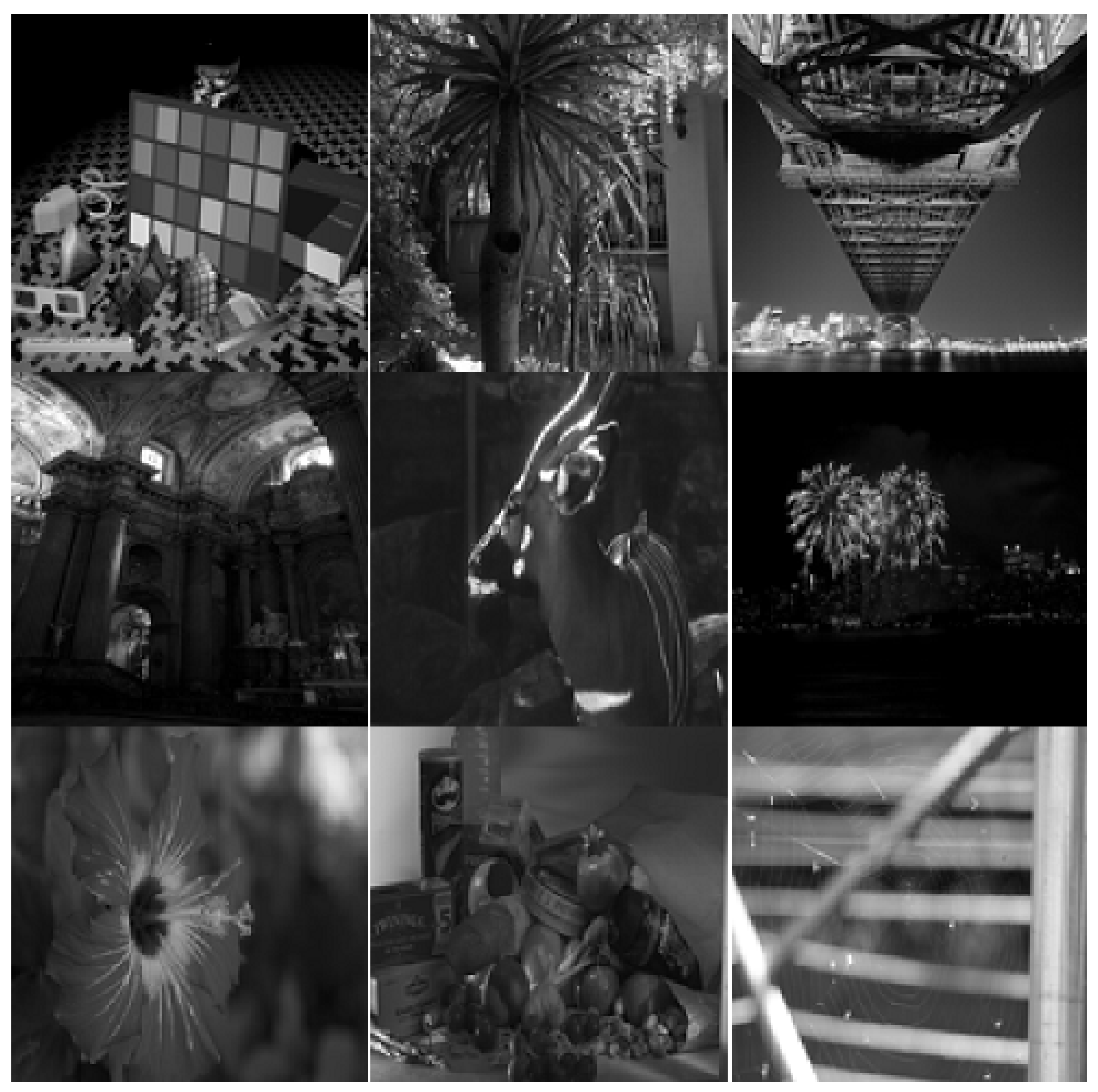
  99. Imagecompression.info. The New Test Images—IMAGE Compression Benchmark. 2020. Available online: https://imagecompression.info/test_images/ (accessed on 10 October 2020).
Figure 1. Steps used to convert a continuous tone image to a digital one.
Electronics 10 00360 g001
Figure 2. An 8-bit greyscale image.
Electronics 10 00360 g002
Figure 3. A 16-bit greyscale image.
Electronics 10 00360 g003
Figure 4. An 8-bit red, green, and blue (RGB) image.
Electronics 10 00360 g004
Figure 5. A 16-bit RGB image.
Electronics 10 00360 g005
Figure 6. An image with the corresponding pixel values.
Electronics 10 00360 g006
Figure 7. A comparison of histograms before and after application of a predictor.
Electronics 10 00360 g007
Figure 8. Basic block diagram of lossless image compression.
Electronics 10 00360 g008
Figure 9. Block diagram for the JPEG-LS encoder [43].
Electronics 10 00360 g009
Figure 10. (a) JPEG 2000 encoder; (b) dataflow [68].
Electronics 10 00360 g010
Figure 11. Dyadic decomposition of a single tile.
Electronics 10 00360 g011
Figure 12. JPEG XR encoder [78].
Electronics 10 00360 g012
Figure 13. JPEG XR decoder [74].
Electronics 10 00360 g013
Figure 14. Examples of 8-bit greyscale images.
Electronics 10 00360 g014
Figure 15. Encoding times for 8-bit greyscale images.
Electronics 10 00360 g015
Figure 16. Decoding times for 8-bit greyscale images.
Electronics 10 00360 g016
Figure 17. Examples of 8-bit RGB images.
Electronics 10 00360 g017
Figure 18. Comparison of encoding times for 8-bit RGB images.
Electronics 10 00360 g018
Figure 19. Comparison of decoding times for 8-bit RGB images.
Electronics 10 00360 g019
Figure 20. Examples of 16-bit greyscale images.
Electronics 10 00360 g020
Figure 21. Comparison of encoding times for 16-bit greyscale images.
Electronics 10 00360 g021
Figure 22. Comparison of decoding times for 16-bit greyscale images.
Electronics 10 00360 g022
Figure 23. Examples of 16-bit RGB images.
Electronics 10 00360 g023
Figure 24. Comparison of encoding times for 16-bit RGB images.
Electronics 10 00360 g024
Figure 25. Comparison of decoding times for 16-bit RGB images.
Electronics 10 00360 g025
Figure 26. Comparison of average compression ratios.
Electronics 10 00360 g026
Figure 27. Comparison of average encoding times.
Electronics 10 00360 g027
Figure 28. Comparison of average decoding times.
Electronics 10 00360 g028
Figure 29. Two-parameter grand total performance (GTP) for 8-bit greyscale images.
Electronics 10 00360 g029
Figure 30. Two-parameter GTP for 8-bit RGB images.
Electronics 10 00360 g030
Figure 31. Two-parameter GTP for 16-bit greyscale images.
Electronics 10 00360 g031
Figure 32. Two-parameter GTP for 16-bit RGB images.
Electronics 10 00360 g032
Figure 33. Three-parameter GTP.
Electronics 10 00360 g033
Table 1. Variable length coding for the image in Figure 6.
Symbol
(S)
Probability
(P(k))
Code-WordCode-Word
Length ( L k )
L k P k
1180.1210030.36
1190.1600130.48
1200.1201130.36
1390.01111140.04
1400.1700030.51
1410.1201030.36
1690.1110130.33
1700.09111040.36
1710.111030.3
L a v g = 3.1 bits
Table 2. Causal template.
EFGPast pixels
HABCCurrent pixel
KDP Future pixels
Table 3. Predictor for Lossless Joint Photographic Experts Group (JPEG).
ModePredictor
0No prediction
1D
2B
3A
4D + BA
5D + (BA)/2
6B + (DA)/2
7(D + B)/2
Table 4. Predictor for Portable Network Graphics (PNG)-based image compression.
Type ByteFilter NamePrediction
0NoneZero
1SubD
2UpB
3AverageThe rounded mean of D and B
4Paeth [56]One of D, B, or A (whichever
is closest to P = D + BA)
Table 5. Comparison of compression ratios for 8-bit greyscale images.
Image Name
(Dimensions)
JPGE-LSJPEG 2000Lossless
JPEG
PNGJPEG XRCALICAVIFWebPFLIF
artificial.pgm
( 2048 × 3072 )
10.0306.7204.8848.6783.19610.8984.14510.37013.260
big_tree.pgm
( 4550 × 6088 )
2.1442.1061.8061.9732.0112.1592.1752.1452.263
bridge.pgm
( 4049 × 2749 )
1.9291.9101.6441.8111.8461.9291.9731.9431.979
cathedral.pgm
( 3008 × 2000 )
2.2412.1601.8132.0152.0382.2542.2222.2172.365
deer.pgm
( 2641 × 4043 )
1.7171.7481.5831.7131.6851.7271.8721.7941.775
fireworks.pgm
( 2352 × 3136 )
5.4604.8533.3554.0953.0545.5164.4864.8585.794
flower_foveon.pgm
( 1512 × 2268 )
3.9253.6502.9703.0542.9323.9354.1153.7493.975
hdr.pgm
( 2048 × 3072 )
3.6783.4212.7952.8572.8473.7183.8253.4563.77
spider_web.pgm
( 2848 × 4256 )
4.5314.2023.1453.3663.1674.8244.6824.1334.876
Table 6. Comparison of compression ratios for 8-bit RGB images.
Image Name
(Dimensions)
JPGE-LSJPEG 2000Lossless
JPEG
PNGJPEG XRCALICAVIFWebPFLIF
artificial.pgm
( 2048 × 3072 )
10.3338.1834.92410.8664.31610.416.88117.38318.446
big_tree.pgm
( 4550 × 6088 )
1.8561.8231.5851.7211.7191.8862.2541.8351.922
bridge.pgm
( 4049 × 2749 )
1.7671.7651.5531.6861.7351.7842.211.7481.866
cathedral.pgm
( 3008 × 2000 )
2.1202.1351.7341.9222.0152.1262.6972.1622.406
deer.pgm
( 2641 × 4043 )
1.5321.5041.4071.5071.4801.5371.9151.5671.588
fireworks.pgm
( 2352 × 3136 )
5.2624.4963.2793.7623.1215.2795.4324.6245.742
flower_foveon.pgm
( 1512 × 2268 )
3.9383.7462.8063.1493.0603.9275.6114.1584.744
hdr.pgm
( 2048 × 3072 )
3.2553.1612.5612.6532.7163.2694.6143.2133.406
spider_web.pgm
( 2848 × 4256 )
4.4114.2093.0293.3653.2344.5556.0174.3174.895
Table 7. Comparison of compression ratios for 16-bit greyscale images.
Image Name
(Dimensions)
JPGE-LSJPEG 2000Lossless
JPEG
PNGJPEG XRCALICAVIFWebPFLIF
artificial.pgm
( 2048 × 3072 )
4.0734.0072.7914.3816.3934.1748.28220.84626.677
big_tree.pgm
( 4550 × 6088 )
1.3551.3251.2871.1814.0281.3244.354.2294.537
bridge.pgm
( 4049 × 2749 )
1.3091.2791.2441.1473.6961.3733.9443.8433.971
cathedral.pgm
( 3008 × 2000 )
1.3731.3371.2931.1914.0841.3424.4504.3984.749
deer.pgm
( 2641 × 4043 )
1.2521.2411.2251.1323.3711.3393.7423.5493.557
fireworks.pgm
( 2352 × 3136 )
1.9461.8091.7401.6046.1161.9558.9679.77311.647
flower_foveon.pgm
( 1512 × 2268 )
1.6101.5911.5231.3165.8841.6638.2737.6268.029
hdr.pgm
( 2048 × 3072 )
1.5951.5631.4911.2975.7551.5697.7797.0407.754
spider_web.pgm
( 2848 × 4256 )
1.7361.7711.5541.3676.3861.7429.6588.44210.196
Table 8. Comparison of compression ratios for 16-bit RGB images.
Image Name
(Dimensions)
JPGE-LSJPEG 2000Lossless
JPEG
PNGJPEG XRCALICAVIFWebPFLIF
artificial.pgm
( 2048 × 3072 )
4.3354.7342.6954.8968.6444.40413.78336.29237.021
big_tree.pgm
( 4550 × 6088 )
1.3021.2611.2491.1503.4411.2844.5043.6143.841
bridge.pgm
( 4049 × 2749 )
1.2741.2431.2401.1323.4701.2834.4143.4453.739
cathedral.pgm
( 3008 × 2000 )
1.3791.3331.2671.2184.0361.3835.3974.2924.851
deer.pgm
( 2641 × 4043 )
1.1971.1731.2361.1002.9611.1963.8263.0963.176
fireworks.pgm
( 2352 × 3136 )
2.3781.8321.6882.0536.4532.38411.31810.04812.283
flower_foveon.pgm
( 1512 × 2268 )
1.7241.6641.4941.3716.1211.76511.2178.3059.513
hdr.pgm
( 2048 × 3072 )
1.5351.5181.4731.2755.4321.5869.2196.3916.819
spider_web.pgm
( 2848 × 4256 )
1.7021.7841.5311.3606.4661.71812.0188.5769.787
Table 9. Summary of results.
Grayscale Images (8 bits)
Compression RatioEncoding TimeDecoding TimeFirst ChoiceSecond Choice
JPEG XRPNG
-JPEG XRJPEG-LS
-PNGLossless JPEG
-JPEG XRPNG
--FLIFCALIC
--PNGLossless JPEG
--JPEG XRJPEG-LS
Grayscale Images (16 bits)
JPEG XRPNG
-JPEG XRFLIF
-PNGJPEG XR
-PNGLossless JPEG
--FLIFWebP
--PNGLossless JPEG
--JPEG XRLossless JPEG
RGB Images (8 bits)
JPEG XRPNG
-JPEG XRJPGE-LS
-PNGJPGE-XR
-JPEG XRPNG
--FLIFWebP
--PNGJPEG XR
--JPEG XRJPEG-LS
RGB Images (16 bits)
JPEG XRPNG
-JPEG XRWebP
-JPEG XRPNG
-JPEG XRPNG
--FLIFWebP
--JPEG XRPNG
--JPEG XRJPEG-LS
Publisher’s Note: MDPI stays neutral with regard to jurisdictional claims in published maps and institutional affiliations.

