Multi-Scale Feature Fusion with Adaptive Weighting for Diabetic Retinopathy Severity Classification

Abstract

Diabetic retinopathy (DR) is the prime cause of blindness in people who suffer from diabetes. Automation of DR diagnosis could help a lot of patients avoid the risk of blindness by identifying the disease and making judgments at an early stage. The main focus of the present work is to propose a feasible scheme of DR severity level detection under the MobileNetV3 backbone network based on a multi-scale feature of the retinal fundus image and improve the classification performance of the model. Firstly, a special residual attention module RCAM for multi-scale feature extraction from different convolution layers was designed. Then, the feature fusion by an innovative operation of adaptive weighting was carried out in each layer. The corresponding weight of the convolution block is updated in the model training automatically, with further global average pooling (GAP) and division process to avoid over-fitting of the model and removing non-critical features. In addition, Focal Loss is used as a loss function due to the data imbalance of DR images. The experimental results based on Kaggle APTOS 2019 contest dataset show that our proposed method for DR severity classification achieves an accuracy of 85.32%, a kappa statistic of 77.26%, and an AUC of 0.97. The comparison results also indicate that the model obtained is superior to the existing models and presents superior classification performance on the dataset.

1. Introduction

Diabetic retinopathy (DR), one of the most common complications of diabetes mellitus, refers to a series of lesions caused by the microvascular damage to the retina resulting from diabetes, and the fundus diseases such as weak vision and blindness in adults are mainly caused by DR. According to relevant statistics, the number of diabetic patients in China will reach 140 million in 2035 [1], which is the country with the most diabetes. In rural China diabetic patients, the prevalence of diabetic retinopathy is 43.1% [2]. According to research, the longer the duration of diabetes, the higher the chance of diabetic retinopathy. Fortunately, DR is a preventable and controllable eye disease. Regular screening is helpful to detect the severity of DR and make an intervention timely, and by this way, if diabetic reticulum disease is recognized at an early stage, many people can avoid blindness [3].

Diabetes will lead to eye problems including glaucoma, cataracts, and DR. Among them, the lesions on the retina of patients with DR include retinal bleeding, microaneurysms, hemorrhages, hard exudates, and cotton wool spots [4]. The doctor’s manual method of directly observing lesion images has a complicated detection process, which puts huge pressure on limited medical resources. The diversity of lesions also makes it difficult to judge the condition of the illness. If the fundus lesion images can be automatically classified in the early stage, it can save a lot of time for patients, which has important research significance. Diabetic retinopathy is a gradual process, according to its severity can be divided into mild, moderate, severe, and value-added diabetes. Microaneurysms will often form in the mildly diseased stage. They grow balloon-like in the retinal veins. If the small retinal blood vessels rupture, a small amount of bleeding will enter the vitreous, and the patient will have dark shadows floating in front of the eyes. In the early stage of proliferation, the patient has more microaneurysm, dilated veins, and cotton wool spots in the retina, which will soon develop into proliferative diabetic retinopathy. In the proliferative stage, the patient’s vitreous hemorrhages, and the eyesight decreases significantly until blindness or weak vision.

In recent years, deep learning technology has demonstrated its important research significance and application value in the field of medical image analysis. For the part of diabetic retinopathy, the initial research focused on the use of traditional machine learning methods to detect macula and the optic disc, make retinal vessel segmentation, and carry out two classifications of diabetes retinopathy. Such as Kayte [5] used SVM to classify images. Gargeya et al. [6] used the residual network and the decision tree classifier to detect the disease. Quellec et al. [7] combined the KNN algorithm with optimal filters, achieving an AUC of 0.927. Then with the development of convolutional neural network (CNN), more network models are used in the classification task of diabetic retinopathy, and the research of automatic classification of DR based on fundus images has received more and more attention from the academic community. On one hand, different from traditional machine learning methods, the convolutional neural network can extract more complex features by increasing the depth of the convolutional layer, and recognize different grades of DR image features through the learning process; on the other hand, it can also combine the feature information of different levels by increasing the width of the neural network. Today, CNN opens a new period in features extraction with high complexity and comprehensiveness, and stands a new height in the DR recognition classification. However, it still faces many new challenges when building an effective and robust DR model with CNN. Actually, in a sense, the results provided by artificial intelligence methods are not explainable. The current research in the medical field through deep learning and other methods is more about assisting doctors to make a diagnosis. In view of the diversity of retinal lesions, it is difficult for the neural network to correspond to a specific lesion or specific lesion type strictly. More neural network models tend to extract useful features from the global image and conduct training classification according to the features. The present work mainly attempts a new approach in the neural network about the extraction of multi-scale features and the adaptive weighting fusion of multi-scale features through the special attention module for retinal lesions. The application test on the APTOS 2019 Kaggle benchmark dataset indicates that the proposed adaptively weighted fusion method in the model improves the identification performance of DR severity and achieves an accuracy of 85.32%, a kappa statistic of 77.26%, and an AUC of 0.97, which performs better than state-of-the-art models. In brief, the main contribution of this work includes:

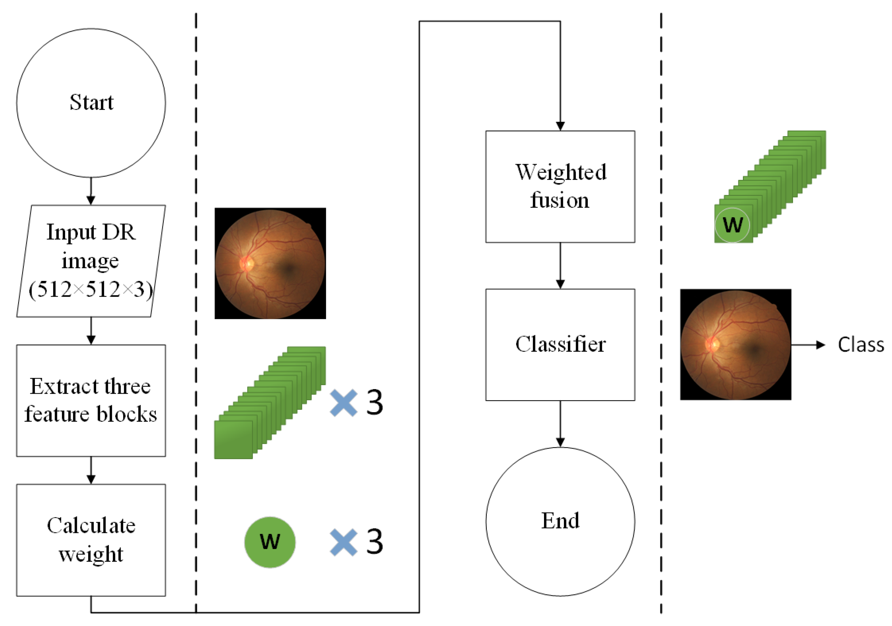
• We design a multi-scale feature extraction method aiming at the classification of DR fundus images and the classification training is carried out by fusing the feature information of different scales in the convolution neural network.
• When fusing the features, we add adaptive weights through the attention module, global average pooling (GAP), and division process, and the weight updates adaptively if each feature block changes with the training of the CNN.
• The classification performance is better than state-of-the-art models on the APTOS 2019 Kaggle benchmark datasets.

2. Related Works

In the last few years, with the development of AI technology, much research on deep learning has been used in the classification task of DR. Early research mainly focused on machine learning algorithms to identify the characteristic parts of the lesion. Soares et al. [8] used filters to extract features and used Bayesian classifiers to segment retinal blood vessels. Srivastava et al. [9] used multi-core processing and combined it with different grid sizes to identify microaneurysms (mas) and hemorrhages (hems) to help the detection of DR classification. Nayak et al. [10] used preprocessing, morphological processing, and texture analysis methods on fundus images to detect features such as exudate area, blood vessel area, and contrast, and then used these features as the input of the artificial neural network (ANN) to classify the fundus images into three categories with an accuracy rate of 93% and a sensitivity of 90%. Adarsh et al. [11] input feature textures such as exudates and microaneurysms into the SVM classification, which classified DR into five categories. Roychowdhury et al. [12] proposed a two-layer classification method and combined four kinds of machine learning algorithms of Gaussian Mixture Model (GMM), k-nearest neighbor (KNN), SVM, and AdaBoost to achieve 100% sensitivity to DR classification, 53.16% specificity, and 0.904 AUC. Priya et al. [13] extracted the characteristics of blood vessels, bleeding, and exudates and input them into the probabilistic neural network (PNN) and SVM for classification. The final accuracy rate of PNN was 89.60%, and the accuracy rate of SVM was 97.608%. Gargeya et al. [6] designed a technology that combines CNN and machine learning algorithms. In this technology, the fundus image and the processed result are used as the input of the residual network, and a small amount of data is added to the fundus image of the previous pooling layer as the input of the decision tree classifier to complete the two classifications.

However, classification by the above traditional machine learning methods relies on a large number of labeled images. Medical workers spend most of their time processing labels instead of diagnosing the state of illness. This process takes a lot of effort and requires additional separation of the prominent part from the entire lesion image, which prevents making more labeled DR images. Moreover, these methods cannot completely cover all the characteristics of DR, and it still takes a lot of time in the follow-up diagnosis and treatment. Nowadays more neural network structures are used in DR classification tasks. Pratt et al. [14] constructed a shallow CNN structure and performed five classifications of DR, and finally reached 95% sensitivity but only 75% accuracy on the verification set. Wang et al. [15] used an attention mechanism to generate the detection frame to obtain the characteristics of the lesion area, simulating the process of real doctors to enlarge the image in clinical diagnosis, and simultaneously diagnosing the diabetic retinopathy and highlighting suspicious areas. It is a better one on performance among the five classification models and is better than other results in the two classifications. Bravo et al. [16] studied the preprocessing method of DR images to improve the performance of the model in the five categories. Zhao et al. [17] improved the model structure based on the work of Bravo et al. in 2019, combining the attention model for feature extraction and the bilinear model for fine-grained classification, meanwhile proposing the grading loss function “Grading Loss” in view of the distance differences between different grades and different classifications, which enables the model to converge faster. Abbas et al. [18] used a semi-supervised deep learning model, without any pre-processing and post-processing of the retinal fundus image and used scale-invariant color-intensive and gradient-direction histogram technology to extract features from each image, completing the DR five classifications with 92.18% sensitivity, 94.50% specificity and 0.924 AUC in the test set.

Recent progress in the extraction of novel features from eye fundus images involves different methods. For example, Orujov et al. [19] used a new approach for retinal vessel segmentation by exploiting the fuzzy logic-based technique and achieved practically usable accuracy on the three datasets. Das et al. [20] applied the technique of maximal principal curvature, which utilizes the maximum Eigenvalues of the Hessian matrix. In order to enhance and eliminate falsely segmented regions, they made an adaptive histogram equalization and morphological opening. Ramasamy et al. [21] extracted and fused the ophthalmoscopic features from the retina images based on textural gray-level features like co-occurrence, run-length matrix, as well as the coefficients of the Ridgelet Transform. Based on the retina features, they used the Sequential Minimal Optimization (SMO) classification to classify the DR images. Most of these feature extraction methods adopted traditional methods, that is, the image followed pre-processing before putting it into the network training. These methods may contain some irrelevant information for DR recognition, which will affect the accuracy of subsequent training and the effect of the model. Therefore, the above methods also have some limitations.

Traditional neural networks mostly use high-level convolution to train fully connected layers to classify diseased images. As is well known, the neural network models have different receptive fields in different training stages. The low-level network feature map has high resolution and a small local receptive field, which may note the small features of the lesion image. The high-level network feature map has a low resolution but a larger receptive field and has a more in-depth representation of the semantic information of the lesion image. Due to the particularity of the retina lesion image, the distribution of the lesion location is different. When the CNN is used to extract the features, the information expressed by each layer is different, and some subtle feature information will disappear if the depth of the network continues to deepen. Today, multi-scale feature extraction technology is widely used in classification networks and target detection. But to the best of our knowledge, there are only limited reports about it being used in DR classification work. For example, Gulshan et al. [22] used a multi-scale feature in Inception-V3 to identify DR. It uses inception to increase the width of the network, extract features of different receptive fields in parallel from the input image and obtain feature information of different scales through different convolution kernels. Kassani et al. [23] proposed a method that is based on deep layer aggregation that combines multilevel features from different convolutional layers of Xception. Nguyen et al. [24] analyzed fundus images with varying illumination and fields of view by VGG-16 and VGG-19. Bodapati et al. [25] extracted and aggregated features from multiple convolution blocks of VGG-16 using pooling and fusion methods. These methods give useful references for our diabetic retinopathy classification model.

In Table 1, we summarized the reported classification results by the above authors.

Table 1. Summary of related work.

Method	Sensitivity	Specificity	Accuracy
Nayak et al. [10]	0.90	1.00	0.93
Adarsh et al. [11]	0.90	0.93	0.95
Roychowdhury et al. [12]	1.00	0.53	-
Priya et al. [13]	0.98	0.96	0.97
Pratt et al. [14]	0.95	-	0.75
Wang et al. [15]	-	-	0.90
Abbas et al. [18]	0.92	0.94	-
Das et al. [20]	0.96	0.95	0.96
Gulshan et al. [22]	0.97	0.93	-
Kassani et al. [23]	0.88	0.87	0.83
Nguyen et al. [24]	0.80	0.82	0.82
Bodapati et al. [25]	-	-	0.84

Different from the existing works, this paper proposes a novel multi-scale feature adaptive weighting fusion classification network, which extracts feature information from different scales through a special attention module, and adds adaptive weights when fusing the features at different layers to complete the DR classification task.

3. Proposed Method

In this work, our purpose is to train a robust DR severity classification model with limited data, which is based on multi-scale feature fusion with adaptive weighting under MobileNetV3 architecture. As has been noted, different feature layers in the neural network model reflect different feature information of the image. The shallow feature map close to the input of the network has a high resolution and small local field of view, which can extract texture features of the image, such as the lines of the diseased image. The middle layer can learn the information that distinguishes image features through training. The high-level feature map of the network has a low resolution but a high field of view, which can effectively extract the semantic feature information of the image. The accuracy of the DR classification task depends on the effectiveness of feature extraction, and we believe that only the high level of the network may not be able to fully express the image features effectively. Our work makes full use of the feature information expressed by different layers and adopts adaptive weighting to fuse multi-layer features. In this way, the shallow features, intermediate features, and deep features are fused to further dig out image information. We hope that this method can extract rich texture information, and at the same time, it can obtain features with better robustness aim at various changes in the image and implement the advantages complementary of the features at different levels, thereby improving the accuracy of DR classification.

However, in the previous multi-scale feature fusion network architecture for classification tasks, some often choose the method of directly adding different scale features together(add), or concat different features(concat), or use designed weight for features when they are integrated (designed weight). These works cannot effectively reflect the proportion of different scale features in the network training, which not only makes the model more bloated but also reduces the recognition accuracy of the model.

In our proposed method, we first choose the 3rd, 4th, and 6th convolutional blocks in the neck as the input of feature fusion, and different from the previous fusing methods of “add”, “concat” or “designed weight”, we propose an adaptively weighted fusion method. The high-level and low-level feature maps are brought closer to the middle layer through different sampling methods to make three convolutional blocks with the same dimensions as the middle layer. Then, the feature extraction is performed through an attention module named RCAM, and meanwhile, to avoid over-fitting of the model and remove non-critical features, the final weight is obtained through global average pooling (GAP) and division operations. Through the above adaptively weighted method, the three convolutional blocks are added together to let the weight of different convolutional layers automatically changed in the model training and achieve the goal of multi-scale feature adaptive weighting fusion of the image. Figure 1 gives the flowchart of the method, and Figure 2 gives the network architectural details of the proposed method.

Figure 1. A flowchart of the proposed method.

Figure 2. Architectures of proposed multi-scale feature classification network with adaptively weighted fusion method.

3.1. Backbone of Model

This paper selects MobileNetV3 [26] proposed by Google in 2019 as the backbone network. Compared with previous neural networks, it has the advantages of faster speed and fewer parameters. Based on the first-generation separable convolutions and the second-generation linear bottleneck residual structure, h-swish is used to replace the swish activation function, and the Squeeze-and-Excitation (SE) lightweight attention module is introduced in this model. This paper chooses the 3rd, 4th, and 6th convolutional blocks of the network neck as the input of multi-scale fusion and obtains three scale sizes of feature maps of 64 × 64 × 40, 32 × 32 × 112, 16 × 16 × 160 through the basic backbone network. In order to solve the invisible problem in the convolutional neural network model, the focus areas of the network model in the input image can be represented by Grad-CAM [27], and the network model can be visualized to intuitively express the reasons for the classification results obtained by the algorithm. It uses feature maps generated from the gradient values of the classification score, $y^c$, with respect to the feature maps, $A_{ij}^k$, in a randomly selected layer. The weight value ${\varpi }_k^c$ is calculated by Equation (1). The visual result is obtained by summing ${\varpi }_k^c$ with the feature map, and the weight ${\varpi }_k^c$ indicates the importance of class c to the feature map.

$${\varpi }_k^c=\frac{1}{z}{\displaystyle \sum }_i{\displaystyle \sum }_j\frac{\partial y^c}{\partial A_{ij}^k}$$

(1)

The influence of negative value on the result of the feature map is removed by the ReLU function, and a heatmap is generated through the formula below.

$$L_{Grad-CAM}^c=ReLU\left({\displaystyle \sum }_k{\varpi }_k^c{A}_{ij}^k\right)$$

(2)

According to the heat map based on the Grad-CAM of DR image shown in Figure 3, we can see that the information reflected by different feature maps in the entire network is different.

Figure 3. Thermal map of the 3rd, 4th, and 6th convolutional blocks.

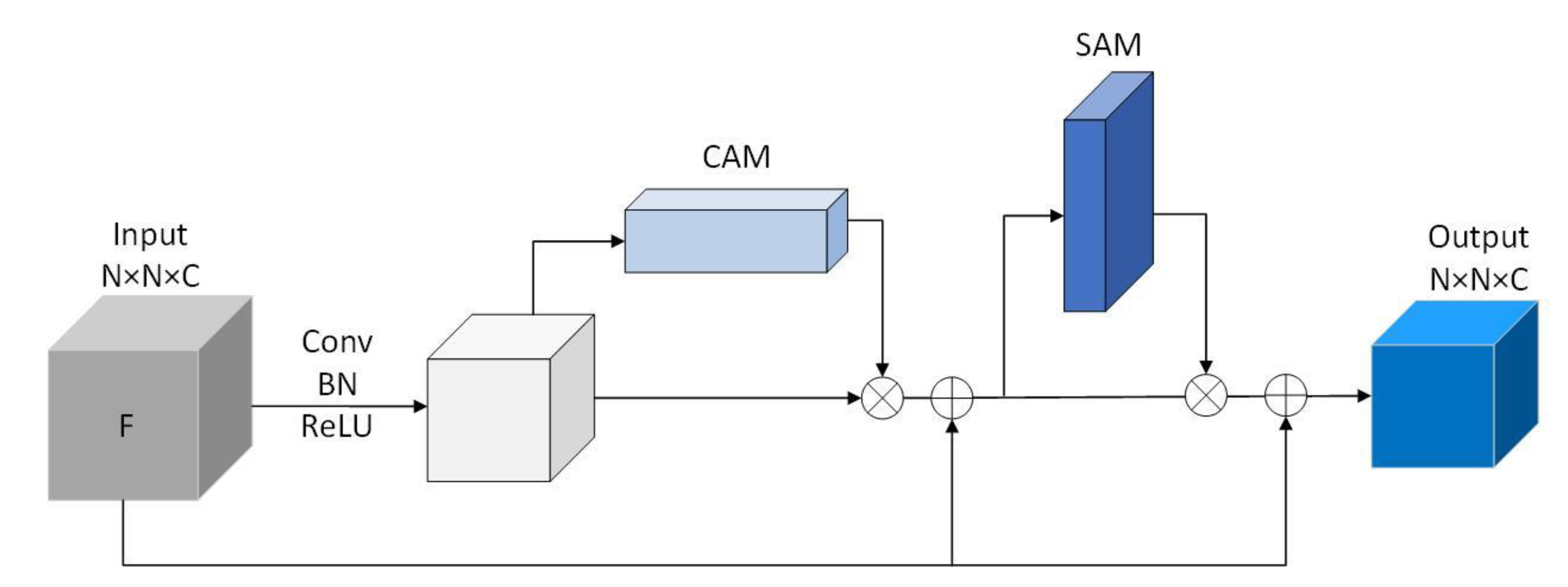
3.2. Residual Convolutional Block Attention Module

Residual Convolutional block Attention Module (RCAM), which connects channel attention module and spatial attention module are designed, and meanwhile, to prevent the gradient from disappearing, the residual module is added in this part. Figure 4 shows the structure of the RCAM module. In the RCAM structure, the original input F of the attention part undergoes a period of 3 × 3 convolutions (Conv), batch normalization (BN), and activation function (ReLU) operations, follows a Channel attention module (CAM) of size 1 × 1 × C and Spatial attention module (SAM) of size N × N × 1 and connects the residual twice. The CAM focuses on the meaningful part of each channel, can deduce information on tiny channels effectively; SAM, as a supplement to CAM, pays more attention to the location of valuable features.

Figure 4. Structure of RCAM module. (The input F is a feature block, the original input F of the attention part undergoes a period of 3 × 3 convolutions (Conv), batch normalization (BN) and activation function (ReLU) operations, follows a Channel attention module (CAM) of size 1 × 1 × C and Spatial attention module (SAM) of size N × N × 1, and connects the residual twice.).

RCAM is computed as:

$$F_C=CAM\left(\mathsf{\Phi }\left({{\displaystyle \sum }}_0^C{{\displaystyle \sum }}_{i,j}^N{X}_{i,j}\cdot W_{i,j}+b\right)\right)\times \mathsf{\Phi }\left({{\displaystyle \sum }}_0^C{{\displaystyle \sum }}_{i,j}^N{X}_{i,j}\cdot W_{i,j}+b\right)$$

(3)

$$F_a=SAM\left(F+F_C\right)+F$$

(4)

among them, Φ is the activation function, F is a convolutional layer of size N × N × C. X represents the input of RCAM, W represents the weight, b represents the bias term, $F_C$ represents the output of CAM, $F_a$ represents the output of RCAM.

3.3. Adaptively Weighted Feature Fusion

Figure 5 shows the structure of adaptively weighted feature fusion. At the left part of Figure 5, the low and high layers are resized to the same size as the middle layer. Then, the channel number of the high-level convolution block is changed through a convolution kernel with a size of 1 × 1 and the up-sampling is made through interpolation. To the low-level convolution block, the down-sampling through a convolution kernel with a size of 3 × 3 and a stride of 2 is performed directly. After these works, three feature maps $F_a$ of the same size were obtained through RCAM.

Figure 5. Structure of adaptively weighted feature fusion.

At the right part, $F_a$ from the 3rd layer is subjected to global average pooling (GAP) and a convolution kernel with a size of 1 × 1 to avoid over-fitting of the model, and then a divide operation to screen out non-critical features, which gets the redistributed weight $F_W$. $F_W$ is computed as:

$$F_W=\frac{F_a}{Conv\left(\frac{1}{H\times W}{{\displaystyle \sum }}_H{{\displaystyle \sum }}_W{F}_a\right)}$$

(5)

Performing the same operation on the other two feature maps will finally get three redistributed weights $F_W^0$, $F_W^1$ and $F_W^2$. Concat the three weights and using softmax, we get the final weights of $W^0$, $W^1$ and $W^2$. The weights $W^i$ is computed as:

$$W^i=\frac{F_W^i}{{{\displaystyle \sum }}_j{F}_W^j}$$

(6)

The weighted feature fusion, at last, is computed as:

$$\mathrm{O}=W^0\cdot F^0+W^1\cdot F^1+W^2\cdot F^2$$

(7)

$F^i$ is the convolutional layer after resizing, and $W^i$ is the weight after adaptive weighting. Algorithm 1 shows the details of the proposed method for DR severity identification.

Algorithm 1 Identification task of DR severity using Adaptively Weighted Fusion

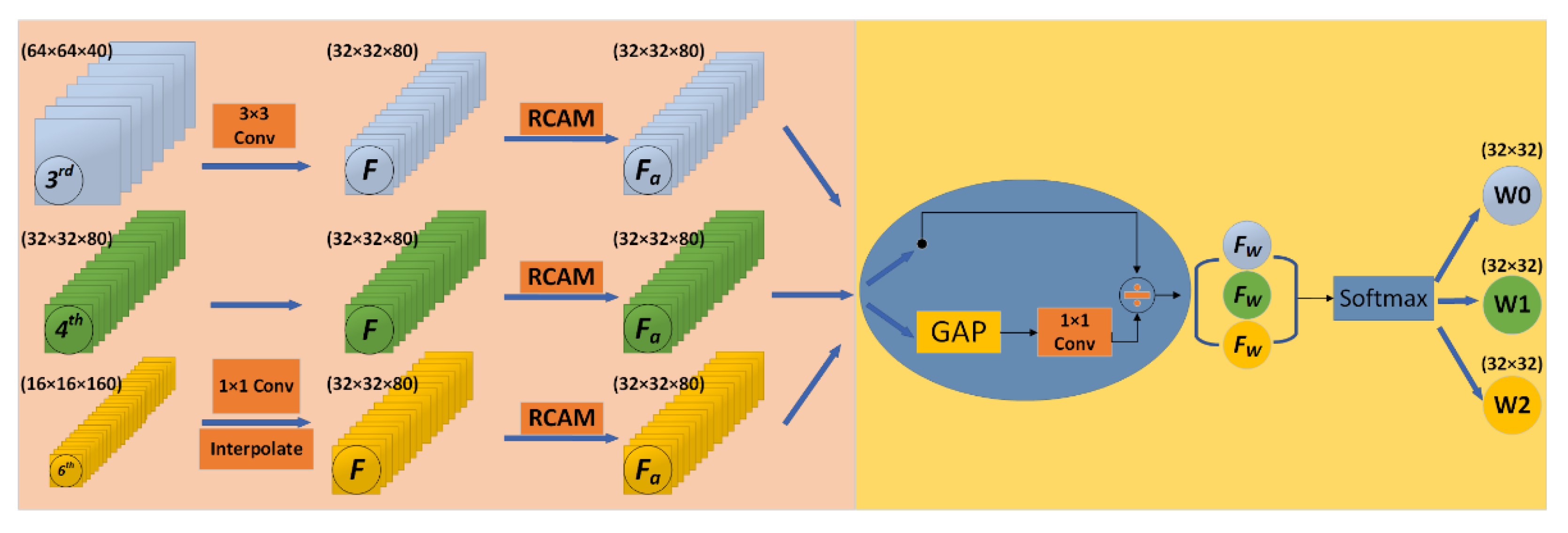
Input: Let $D^{Tr}$ and $D^{Tst}$ be the train dataset and test dataset of DR images, where $D^{Tr}=\left\{{\left(x_i,y_i\right)}_{i=1}^{N_{Tr}}\right\} \mathrm{and} D^{Tst}=\left\{{\left(x_i\right)}_{i=1}^{N_{Tst}}\right\}$. $x_i$ represents $i$th color fundus image in the dataset and $y_i$ is the severity level of DR associated with $x_i$. In the case of the DR classification task, $y_i\in \left\{0,1,2,3,4\right\}$. Output: $y_i$ for each $x_i\in D^{Tst}$ Step 1: Preprocess each image $x_i$ in the dataset. Step 2: Feature Extraction For each preprocessed image $x_i$, three different features ($F^{l3}$,$F^{l4}$,$F^{l6}$) are extracted.  $F^{l3}\leftarrow$ Feature extracted from third bottleneck layer block of MobileNet  $F^{l4}\leftarrow$ Feature extracted from fourth bottleneck layer block of MobileNet  $F^{l6}\leftarrow$ Feature extracted from sixth bottleneck layer block of MobileNet Where dimensions (W $\times$ H $\times$ C) of $F^{l3}$, $F^{l4}$ and $F^{l6}$ are 64 $\times$ 64 $\times$ 40, 32 $\times$ 32 $\times$ 80 and 16 $\times$ 16 $\times$ 160, respectively. Step 3: Feature Resizing resize the features($F^{l3}$and$F^{l6}$) to the same shape of the feature($F^{l4}$). For $F^{l3}$, apply a 1 $\times$ 1 convolution layer to compress the number of channels and then upscale with interpolation. For $F^{l6}$, apply a 3 $\times$ 3 convolution layer with a stride of 2. Step 4: Adaptively Weighted Fusion Let $F_R^1$, $F_R^2$ and $F_R^3$ be the resized feature, and let $F_a^i$ be the feature extracted from attention block(RCAM) For each $F_a^i\in \left\{RCAM(F_R^i)\right\}$  $F_W^i=\frac{F_a^i}{Conv\left(\frac{1}{H\times W}{{\displaystyle \sum }}_H{{\displaystyle \sum }}_W{F}_a^i\right)}$  $W^i=\frac{F_W^i}{{{\displaystyle \sum }}_j{F}_W^j}$  $\mathrm{O}={\displaystyle \sum }_i{F}^i\cdot W^i$ Let O be the merged representation. Step 5: Model Training Training dataset is prepared using the blended features $D^{Tr}=\left\{{\left(\widehat{x_i},y_i\right)}_{i=1}^{N_{Tr}}\right\}$, where $\widehat{x_i}$ is the feature representation of $x_i$, and $y_i$ is the output of the softmax classifier. Train a deep neural network (DNN) using $D^{Tr}$ Step 6: Model evaluation The test dataset is prepared using the blended features $D^{Tst}=\left\{{\left(\widehat{x_i}\right)}_{i=1}^{N_{Tst}}\right\}$ Evaluate the performance of $D^{Tst}$ using the DNN in Step 5

3.4. Loss

Using the above-mentioned multi-scale feature extraction and adaptively weighted fusion method, the finally obtained feature layer is input into the classification model, and the DR image is divided into 5 categories by the softmax function at the end. Batch normalization is used to avoid over-fitting, and a dropout of 0.3 is applied to the input neurons. Dropout can not only solve the phenomenon of overfitting in the training model but also has less training time due to reducing the complexity of the network structure [28]. However, due to the extremely unbalanced distribution of the DR dataset that the fundus images without disease are far more than those with DR, the previous loss functions such as the cross-entropy loss function cannot distinguish the distance of categories because of the same weight of each sample and therefore give a bad result between the DR images. In order to improve the train speed and reduce the loss of accuracy, here we choose Focal Loss [29] as the loss function. Focal Loss is computed as

$${ℒ}_{FL}\left(\widehat{y},y\right)=-{{\displaystyle \sum }}_{i=1}^{n=5}{y}_i\alpha {\left(1-\widehat{y_i}\right)}^{\gamma }·\mathit{log}\widehat{y_i}$$

(8)

Being α a weighing factor and γ the so-called focusing parameter that penalizes errors in wrongly classified examples more than errors in correctly classified ones. $\widehat{y}$ is the prediction result and y is the corresponding label.

4. Experimental Results

In this section, we provide some details of experimental studies obtained from the DR classification task based on the proposed model. The model is trained on an AMD Ryzen 9 CPU which has 12 cores and an RTX3090 GPU, using Adam optimizer and dynamical adjustment of the learning rate until parameters are no longer updated. The initial learning rate is 0.001.

4.1. Dataset Summary

We benchmark the proposed model on the Kaggle dataset released as part of the APTOS 2019 Blind Detection Challenge [30]. This Kaggle dataset is an extensive collection of retinal fundus images, using fundus photography through different imaging conditions. The retinal images were taken over a long period of time through scanners in different clinics. The images were manually assigned to one of five severity levels of retinopathy in diabetic patients. Table 2 lists the number of DR images at different levels in the dataset.

Table 2. Summary of the Kaggle APTOS 2019 challenge dataset for DR severity classification.

Level of Severity	Samples
Normal (class-0)	1805
Mild (class-1)	370
Moderate (class-2)	999
Severe (class-3)	193
Proliferate (class-4)	295

As we can see, this dataset has an imbalance with much more images in class 0 and very few images in class 3. In all experiments, we assess the performance of the DR classification task through training and testing, and the 8:2 ratio was applied to the dataset. And for effective computation of features, all images are resized to 512 × 512 pixels. Figure 6 shows the different images in each category.

Figure 6. Different categories of DR severity images.

4.2. Performance Measures

In this paper, we use accuracy, precision, recall, and F1 score to demonstrate the efficacy of the proposed method. Moreover, we used the Kappa statistic to compare an observed accuracy with an expected accuracy. Kappa statistic is calculated as

$$\mathrm{Kappa}\mathrm{Score}=\frac{\left(\mathrm{Observed}\mathrm{Accuracy}-\mathrm{Expected}\mathrm{Accuracy}\right)}{\left(1-\mathrm{Expected}\mathrm{Accuracy}\right)}$$

(9)

where observed accuracy is the relative observed agreement among raters, and expected accuracy is the hypothetical probability of chance agreement.

4.3. Result Analysis and Discussion

This part focuses on building a DR classification model with accurate classification and high robustness. For the model proposed, we divided our research into different tasks. First of all, we explore the different combinations of convolution blocks for different fusion approaches and show a visualization of our convolution layers as well as the thermal map under MobileNetv3 and our proposed network. Then we compared the impact of different weights calculation methods and fusion methods. Finally, through comparing with the state-of-the-art model to prove the effectiveness of the proposed model.

4.3.1. Comparison of Different Blocks Combination for Fusion Approaches

In this work, we first compared the effect when chooses different convolution block combinations with different fusion methods on the experimental results, and then, we show the visualization analysis of the model convolution layers.

As previously mentioned, each layer of the network output convolutional layer contains different information. Those close to the input layer have more macro features, and the convolution block close to the output layer retains local features that are more useful for DR detail classification. Table 3 shows the ability to select different multiple convolutional blocks to distinguish DR images through simple addition feature fusion and the proposed method. It can be seen from Table 3 that what we choose (the 3rd, 4th, and 6th blocks) in our proposed method is more effective than other combinations and presents a preferable performance from Kappa and F1 Score values. The model proposed leads to an accuracy of 85.32%, which is also better than others.

Table 3. Performance of proposed method with other different blocks for feature fusion.

Convolution Block	Accuracy	Kappa Score	F1 Score
3 and 4 (add)	58.33%	47.22%	57.15%
3 and 5 (add)	67.28%	56.41%	67.22%
3 and 6 (add)	73.37%	64.24%	73.21%
4 and 5 (add)	69.35%	58.89%	69.37%
4 and 6 (add)	75.84%	67.92%	75.81%
3, 4 and 5 (add)	79.98%	70.87%	79.93%
3, 4 and 5 (proposed)	83.15%	72.87%	83.11%
3, 4 and 6 (add)	83.51%	74.65%	83.48%
3, 4 and 6 (proposed)	85.32%	77.26%	85.30%

The visualization effects of different convolution layers of the 3rd, 4th, and 6th in MobileNetV3 and the model proposed are as shown in Figure 7. The first column is the original DR image, the second column is the visualization of different convolutional blocks and the heat map of the classifier layer under MobileNetV3, and the third is the corresponding visualization and thermal map under our network. For different convolution blocks, we choose one of the channels as a visual example. And the heat map is drawn through Grad-Cam. For better display, we have adjusted them to a uniform size. The black and white image is corresponding to the channel of the selected convolution block, and then we select the tensor at the first channel for visualization. The heat map is the visual result obtained by mapping the network classification score back to the corresponding network layer through the backward.

Figure 7. Visualization of different convolution layers between the MobileNetV3 and the proposed networks.

From the first three lines, we can see that under the influence of adaptive weights, the white points (feature numbers) decrease compared with the original network, but the main features identified in the MobileNetV3 did not disappear in the proposed method. We believe that the reduction in feature counts is due to the operation of “attention and division” in our RCAM to remove redundant information. And from the comparison between the original image and the heat map in the last line, we can see that the focus of the adaptive weighted network after attention module and division operation is different from that of the MobileNetV3 observably. In conclusion, the network model after adaptive weighting fusion retains the main features of each layer, and pays attention to features that are not noticed by the original network at the edge of the image, which makes some pathological features more prominent.

4.3.2. Performance Comparison of Different Weights Calculating Methods and Fusion Methods

We also compared different methods of calculating weights: 1 × 1 convolution kernel, 3 × 3 convolution kernel, and RCAM. From Table 4, we can know that our proposed method is better than the other two weight calculation methods. And the effect of using the 1 × 1 convolution kernel is better than the 3 × 3 convolution kernel. We think the reason is that the 3 × 3 convolution kernel loses some information compared with the 1 × 1 kernel in the process of extracting features.

Table 4. Different methods of calculating weight.

Calculate Weight	Accuracy	Kappa Score
Model (with 1 $\times$ 1 Conv)	84.51%	76.61%
Model (with 3 $\times$ 3 Conv)	83.87%	75.34%
Model (with RCAM)	85.32%	77.26%

Meanwhile, the performance among different fusion methods (add, concat, designed weight, and adaptive weight) were compared in Table 5. It shows that the multi-scale feature fusion method we proposed with adaptive weighting is superior to other models in accuracy and kappa.

Table 5. Different methods of feature fusion.

Fusion Method	Accuracy	Kappa Score
Model (add)	83.51%	74.65%
Model (concat)	80.25%	70.81%
Model (designed weight) 1	83.89%	73.44%
Model (proposed)	85.32%	77.26%

¹ The 3rd, 4th, and 6th Conv blocks are weighted in a ratio of 2:3:5.

Furtherly, we give Figure 8 to depict the class-wise, micro-, and macro-AUC values for the proposed model. Although the ROC curve is usually applicable to binary classification, it can be extended to multi-classification problems in a one-to-many way. For example, the diabetic retinopathy classification task has five categories: 0, 1, 2, 3, and 4. When we need to generate a ROC curve of class 0, we can consider class 0 as the positive category, and the other four categories can be treated as a negative class. The ROC curve of every other class can be treated as a similar dichotomy problem. AUC is obtained by calculating the area under the ROC curve. The result achieves 0.97 micro-AUC and 0.95 macro-AUC.

Figure 8. ROC curve for the proposed method.

4.3.3. Computational Complexity Comparison of the Proposed Method with Others

In this experiment, we compared the computational complexity of the proposed method with other CNNs. The input image size is set to 512 $\times$ 512 $\times$ 3. Params are the parameters of the model, Madds are the theoretical amount of multiply-adds, and FLOPs are the theoretical amount of floating-point arithmetics. Table 6 shows that although Params, Madds, and FLOPs have increased compared to the original backbone network of MobileNetV3 and MobileNetV2, they are still lightweight compared to other CNNs.

Table 6. Computational complexity comparison.

Model	Parameters	Madds	FLOPs
Vgg-16	5.481 M	160.7 G	80.48 G
ResNet-50	25.5 M	42.93 G	21.5 G
Inception-V3	23.8 M	35.1 G	17.5 G
Xception	9.5 M	25.08 G	12.6 G
MobileNetV2	3.5 M	3.27 G	1.67 G
MobileNetV3	4.2 M	2.32 G	1.18 G
Proposed	6.78 M	5.83 G	3.54 G

4.3.4. Performance Comparison of the Proposed Method with State of the Art

In this experiment, we compared the model proposed with the state-of-the-art DR severity classification model and proved the effectiveness of our adaptively weighted fusion network of DR severity classification. Table 7 shows the performance comparison between the model obtained and the models used in [23,24,25]. We can see that the performance evaluation of the proposed method in this paper is significantly better than the existing models in the literature. Compared with the model using VGG with feature fusion in [25], we also achieved 0.97 on AUC but improved accuracy and kappa score.

Table 7. Comparison of the proposed method with state-of-the-art models.

Model	Accuracy	AUC	Kappa Score
ResNet50 [23]	74.6%	-	-
Inception V3 [23]	78.7%	-	-
MobileNet [23]	79.0%	-	-
Xception [24]	79.5%	-	-
VGG [24]	82.0%	-	-
Modified Xception [23]	83.0%	0.92	-
Modified VGG [25]	84.3%	0.97	75.87%
Proposed	85.3%	0.97	77.26%

Figure 9 shows the confusion matrix when our model is applied to the DR severity prediction task. The horizontal axis represents the predicted value and the vertical axis represents the true label. One can see that, most of each category is predicted to the correct position, except for the Severe DR type (class-3) images and Proliferate DR type (class-4) images: a part of the Severe DR type images about 29% is incorrectly distinguished as the third and fifth categories, and a part of the Proliferate DR type images about 32% is classified as moderate. In general, the model presents excellent classification performance of DR detection, and the first category (No DR) is the easiest to detect, while the fifth category (Proliferate DR type) is the most difficult to classify.

Figure 9. Confusion matrix for the severity prediction task.

5. Discussion

The proposed method for DR severity classification by multi-scale feature fusion with adaptive weighting achieves good results on the Kaggle dataset and is comparable to the SOTA, which provides an idea of multi-scale feature extraction for medical image and DR automatic diagnosis. However, the proposed method also has some limitations, The results provided by artificial intelligence methods are inexplicable, for example in the part of weight extraction, weights extracted through attention module, GAP, and division operations may still contain unrelated features. Moreover, due to a large number of convolution layers in the middle of the model, the computational complexity and operation time of the model are increased. These limitations can be overcome by further improving the fusion operation of intermediate features and implementing lightweight design for the network architecture.

6. Conclusion and Future Work

The objective of this paper is to establish an effective and robust DR severity classification model with limited data. In the research, we propose a novel multi-scale feature fusion network for DR classification based on MobileNet. Our model extracts feature weights by special attention module RCAM and implements the adaptively weighted fusion of different original convolution blocks. The experimental results show that the proposed method is effective for the fusion of different convolutional layers and can significantly fuse the feature maps of different depths. Compared with the original MobileNetV3 and some other SOTA algorithms on the Kaggle dataset containing 3662 images in total, the proposed network model has achieved better results (we achieved 85.32% accuracy, 77.26% kappa statistic, and 97% AUC), which provides a feasible way for DR severity classification by multi-scale feature fusion and presents an application potential to some extent. In the future, we will improve the feature fusion operation to reduce the computational complexity, and explore different fusion methods to improve the accuracy of the classification model suitable for a DR diagnosis handheld device. In addition, because any AI black box diagnostics systems are not accepted by a professional ophthalmologist in the real world, regardless of their fine results, the current researches in the medical field through deep learning neural network are more about assisting doctors to make a diagnosis. We will further explore how much help our model can provide clinicians, and shorten the distance of the model from DR specialists.

References

1. Guariguata, L.; Whiting, D.R.; Hambleton, I.; Beagley, J.; Linnenkamp, U.; Shaw, J.E. Global estimates of diabetes prevalence for 2013 and projections for 2035. Diabetes Res. Clin. Pract. 2014, 103, 137–149. [Google Scholar] [CrossRef] [PubMed]
2. Wang, F.H.; Yuan, B.L.; Feng, Z.; Wang, J.J. Prevalence of Diabetic Retinopathy in Rural China: The Handan Eye Study. Ophthalmology 2009, 116, 461–467. [Google Scholar] [CrossRef] [PubMed]
3. Doshi, D.; Shenoy, A.; Sidhpura, D.; Gharpure, P. Diabetic retinopathy detection using deep convolutional neural networks. In Proceedings of the 2016 International Conference on Computing, Analytics and Security Trends (CAST), Pune, India, 11 July 2016. [Google Scholar]
4. Williams, R.; Airey, M.; Baxter, H.; Forrester, J.; Kennedy-Martin, T.; Girach, A. Epidemiology of diabetic retinopathy and macular oedema: A systematic review. Eye 2004, 18, 963–983. [Google Scholar] [CrossRef] [PubMed]
5. Kayte, S. Automated diagnosis non-proliferative diabetic retinopathy in fundus images using support vector machine. Inter.-Natl. J. Comput. Appl. 2015, 125, 4. [Google Scholar]
6. Gargeya, R.; Leng, T. Automated Identification of Diabetic Retinopathy Using Deep Learning. Ophthalmology 2017, 124, 962–969. [Google Scholar] [CrossRef] [PubMed]
7. Quellec, G.; Russell, S.; Abramoff, M. Optimal Filter Framework for Automated, Instantaneous Detection of Lesions in Retinal Images. IEEE Trans. Med. Imaging 2010, 30, 523–533. [Google Scholar] [CrossRef] [PubMed]
8. Soares, J.V.B.; Leandro, J.J.G.; Cesar, R., Jr.; Jelinek, H.F.; Cree, M.J. Retinal vessel segmentation using the 2-D Gabor wavelet and supervised classification. IEEE Trans. Med. Imaging 2006, 25, 1214–1222. [Google Scholar] [CrossRef] [PubMed]
9. Srivastava, R.; Duan, L.; Wong, D.W.; Liu, J.; Wong, T.Y. Detecting retinal microaneurysms and hemorrhages with robustness to the presence of blood vessels. Comput. Methods Programs Biomed. 2017, 138, 83–91. [Google Scholar] [CrossRef] [PubMed]
10. Nayak, J.; Bhat, P.S.; Acharya, R.; Lim, C.M.; Kagathi, M. Automated identification of diabetic retinopathy stages using digital fundus images. J. Med. Syst. 2008, 32, 107–115. [Google Scholar] [CrossRef] [PubMed]
11. Adarsh, P.; Jeyakumari, D. Multiclass SVM-based automated diagnosis of diabetic retinopathy. In Proceedings of the 2013 International Conference on Communication and Signal Processing, Melmaruvathur, India, 3–5 April 2013. [Google Scholar]
12. Roychowdhury, S.; Koozekanani, D.D.; Parhi, K.K. DREAM: Diabetic Retinopathy Analysis Using Machine Learning. IEEE J. Biomed. Health Inform. 2014, 18, 1717–1728. [Google Scholar] [CrossRef] [PubMed]
13. Priya, R.; Aruna, P. SVM and Neural Network based Diagnosis of Diabetic Retinopathy. Int. J. Comput. Appl. 2012, 41, 6–12. [Google Scholar] [CrossRef]
14. Pratt, H.; Coenen, F.; Broadbent, D.M.; Harding, S.P.; Zheng, Y. Convolutional neural networks for diabetic retinopathy. Procedia Comput. Sci. 2016, 90, 200–205. [Google Scholar] [CrossRef]
15. Wang, Z.; Yin, Y.; Shi, J.; Fang, W.; Li, H.; Wang, X. Zoom-in-Net: Deep Mining Lesions for Diabetic Retinopathy Detection. In Proceedings of the International Conference on Medical Image Computing and Computer-Assisted Intervention 2017, Quebec City, QC, Canada, 11–13 September 2017; pp. 267–275. [Google Scholar]
16. Bravo, M.A.; Arbelaez, P. Automatic diabetic retinopathy classification. In Proceedings of the 13th International Conference on Medical Information Processing and Analysis, San Andres Island, Colombia, 5–7 October 2017; p. 105721. [Google Scholar]
17. Zhao, Z.; Zhang, K.; Hao, X.; Tian, J.; Chua, M.C.H.; Chen, L.; Xu, X. BiRA-Net: Bilinear Attention Net for Diabetic Retinopathy Grading. In Proceedings of the 2019 IEEE International Conference on Image Processing (ICIP), Taipei, Taiwan, 22–25 September 2019; pp. 1385–1389. [Google Scholar]
18. Abbas, Q.; Fondon, I.; Sarmiento, A.; Jiménez, S.; Alemany, P. Automatic recognition of severity level for diagnosis of diabetic retinopathy using deep visual features. Med. Biol. Eng. Comput. 2017, 55, 1959–1974. [Google Scholar] [CrossRef] [PubMed]
19. Orujov, F.; Maskeliūnas, R.; Damaševičius, R.; Wei, W. Fuzzy based image edge detection algorithm for blood vessel detection in retinal images. Appl. Soft Comput. 2020, 94, 106452. [Google Scholar] [CrossRef]
20. Das, S.; Kharbanda, K.; Raman, R. Deep learning architecture based on segmented fundus image features for classification of diabetic retinopathy. Biomed. Signal. Process. Control. 2021, 68, 102600. [Google Scholar] [CrossRef]
21. Ramasamy, L.K.; Padinjappurathu, S.G.; Kadry, S.; Damaševičius, R. Detection of diabetic retinopathy using a fusion of textural and ridgelet features of retinal images and sequential minimal optimization classifier. PeerJ Comput. Sci. 2021, 7, e456. [Google Scholar] [CrossRef] [PubMed]
22. Gulshan, V.; Peng, L.; Coram, M.; Stumpe, M.C.; Wu, D.; Narayanaswamy, A.; Venugopalan, S.; Widner, K.; Madams, T.; Cuadros, J.; et al. Development and Validation of a Deep Learning Algorithm for Detection of Diabetic Retinopathy in Retinal Fundus Photographs. JAMA 2016, 316, 2402–2410. [Google Scholar] [CrossRef] [PubMed]
23. Kassani, S.H.; Kassani, P.H.; Khazaeinezhad, R.; Wesolowski, M.J.; Schneider, K.A.; Deters, R. Diabetic retinopathy classifi-cation using a modified xception architecture. In Proceedings of the 2019 IEEE International Symposium on Signal Processing and Information Technology (ISSPIT), Ajman, United Arab Emirates, 10–12 December 2019; pp. 1–6. [Google Scholar]
24. Nguyen, Q.H.; Muthuraman, R.; Singh, L.; Sen, G.; Tran, A.C.; Nguyen, B.P.; Chua, M. Diabetic Retinopathy Detection using Deep Learning. In Proceedings of the 4th International Conference on Machine Learning and Soft Computing; ACM, Haikou, China, 15–17 January 2022; pp. 103–107. [Google Scholar]
25. Bodapati, J.D.; Shaik, N.S.; Naralasetti, V. Deep convolution feature aggregation: An application to diabetic retinopathy se-verity level prediction. Signal Image Video Process. 2021, 1–8. [Google Scholar] [CrossRef]
26. Howard, A.; Sandler, M.; Chen, B.; Wang, W.; Chen, L.-C.; Tan, M.; Chu, G.; Vasudevan, V.; Zhu, Y.; Pang, R.; et al. Searching for MobileNetV3. In Proceedings of the 2019 IEEE/CVF International Conference on Computer Vision (ICCV), Seoul, Korea, 27 October–2 November 2019; pp. 1314–1324. [Google Scholar]
27. Selvaraju, R.R.; Cogswell, M.; Das, A.; Vedantam, R.; Parikh, D.; Batra, D. Grad-cam: Visual explanations from deep net-works via gradient-based localization. In Proceedings of the IEEE International Conference on Computer Vision, Venice, Italy, 22–29 October 2017; pp. 618–626. [Google Scholar]
28. Srivastava, N.; Hinton, G.; Krizhevsky, A.; Sutskever, I.; Salakhutdinov, R. Dropout: A Simple Way to Prevent Neural Networks from Overfitting. J. Mach. Learn. Res. 2014, 15, 1929–1958. [Google Scholar]
29. Lin, T.-Y.; Goyal, P.; Girshick, R.B.; He, K.; Dollar, P. Focal Loss for Dense Object Detection. IEEE Trans. Pattern Anal. Mach. Intell. 2020, 42, 318–327. [Google Scholar] [CrossRef] [PubMed]
30. Kaggle Diabetic Retinopathy Detection Competition. Available online: https://www.kaggle.com/c/aptos2019-blindness-detection (accessed on 19 March 2021).
Publisher’s Note: MDPI stays neutral with regard to jurisdictional claims in published maps and institutional affiliations.
Article Metrics
Citations
Article Access Statistics
Multiple requests from the same IP address are counted as one view.