Abstract
In this paper, we propose a two-layer data hiding method by using the Hamming code to enhance the hiding capacity without causing significantly increasing computation complexity for AMBTC-compressed images. To achieve our objective, for the first layer, four disjoint sets using different combinations of the mean value (AVG) and the standard deviation (VAR) are derived according to the combination of secret bits and the corresponding bitmap, following Lin et al.’s method. For the second layer, these four disjoint sets are extended to eight by adding or subtracting 1, according to a matrix embedding with (7, 4) Hamming code. To maintain reversibility, we must return the irreversible block to its previous state, which is the state after the first layer of data is embedded. Then, to losslessly recover the AMBTC-compressed images after extracting the secret bits, we use continuity feature, the parity of pixels value, and the unique number of changed pixels in the same row to restore AVG and VAR. Finally, in comparison with state-of-the-art AMBTC-based schemes, it is confirmed that our proposed method provided two times the hiding capacity comparing with other six representative AMBTC-based schemes while maintaining acceptable file size of steog-images.
1. Introduction
Due to the openness of the Internet, transmitted messages are now at greater risk of being tampered with or compromised [1]. Therefore, mechanisms must be developed to protect transmitted messages, especially sensitive information such as medical and military data. Data hiding conceals secret information in a cover carrier so that the hidden data is not easily detected by malicious attackers [2]. Digital images often serve as cover media because they are easy to obtain and contain multiple redundant pixel values or features for carrying confidential data. Once the embedding operation is done, the hidden image is called a ‘steog-image’ [3].
Data hiding techniques for images can generally be classified into three domains: spatial, transformation, and compression. A spatial domain-based data hiding scheme is one that embeds confidential messages into a cover image by simply modifying its pixel values. A representative scheme is least significant bit (LSB) substitution [4]. Following LSB substitution, many schemes based on histogram shifting have been proposed [5,6]. The frequency domain-based information hiding method transforms a cover image into frequency coefficients by means of a discrete wavelet transform (DWT) [7], discrete transform (DCT) [8], etc. Secret data is embedded into coefficients, then the inverse operation is conducted to obtain the steog-image. In general, transform domain-based data hiding schemes are stronger at resisting malicious attacks than spatial domain-based schemes, but at the cost of computational complexity. To extend the applications of data hiding, compression domain schemes are proposed. Conventional compression techniques are explored, such as vector quantization (VQ) [9], side match vector quantization (SMVQ) [10], block truncation coding (BTC) [11], and Joint Photographic Experts Group (JPEG) [12]. Among them, Lema and Mitchell’s absolute moment block truncation coding (AMBTC) [13] has attracted scholarly attention in the past decade because its computation is more efficient than other BTC variants while maintaining similar quality of the reconstructed image.
BTC or AMBTC family-based data hiding schemes can be further classified into four categories according to what kind of technologies they co-work with [14]: (1) histogram shifting (HS) based [15,16,17,18]; (2) block classification based [14,19,20,21,22]; (3) prediction error expansion (PEE) based [23,24,25,26,27,28,29]; or (4) Type 1 based [28,29,30,31,32] data hiding methods:
- (1)
- The HS-based method, as given by Li et al. [15], proposed a reversible data hiding (RDH) scheme for BTC-compressed images by using bitmap flipping and HS strategies for two-level quantizers. Subsequently, some methods based on HS were proposed [16,17,18]. Due to the lack of additional information in the stego bit stream, low image distortion is achieved when data is embedded; however, the data capacity is low.
- (2)
- The block classification-based method, as first developed by Chuang and Chang [19] in 2006. For a given cover image, it is encoded by BTC and then blocks are classified as smooth or complex ones by using predefined thresholds. The secret bits are embedded into the bitmaps of the selected BTC-compressed blocks. Later, scholars developed variant methods [20,21,22] based on Chung and Chang’s idea.
- (3)
- Sun’s PEE-based method [24], in which a joint neighbor coding (JNC) technique is used to encode BTC-compressed data according to the secret bits. All high average values and low mean values of BTC-compressed blocks are collected as the high mean table and low mean table, respectively. Two secret bits are embedded into each value of either high mean table or low mean table. In general, Sun’s method obtains a capacity four times greater than the number of blocks in the cover image at the cost of extra data to be included in the stego BTC compression stream. It also requires a special BTC-decoding algorithm to derive the reconstructed image. In 2017, Hong et al. [25] modified the prediction and classification rules of Sun et al. and proposed an improved method with a lower bit rate. However, their method also needs two-bit indicators to represent four types of prediction errors. Using a fixed-size indicator may not be effective in representing coding conditions because it leads to an increased bit rate. To overcome these shortcomings of negative prediction errors, in 2018, Chang et al. also adopted the ideas of Sun et al. and used JNC to embed secret information by an exclusive OR operator [27]. At the same year, Hong et al. used a reversible integer transform method to represent their two-level quantizers based on their mean and difference values [28]. In addition, the prediction error is further classified as a symmetrical coding case by using the adaptive classification method. Experimental results confirm Hong et al.’s method provides the lowest bit rate than previous methods.
- (4)
- Type 1-based methods hide confidential data by modifying the AMBTC codes. For example, in 2014, Pan et al. [32] designed a reference matrix and used different combinations of two quantizer. Then, four cases are designed for data hiding based on different combinations of two quantifiers, the high mean value (H) and low mean value (L) in each block. In the next year, Lin et al. designed another data hiding method by modified high and low means of AMBTC blocks [31]. In Lin et al.’s method, four disjoint sets are created as embeddable blocks, in which the unique number of pixels in each block is more than 2 to embed secret data via different combinations of the mean value (AVG) and the standard deviation (VAR). Experimental results confirm that Lin et al.’s method offers high hiding capacity based on their unique data hiding strategy. As for Zhang et al.’s [33] and Huynh et al.’s [34], both schemes took the similar strategies to hide secret data by modifying the AMBTC codes.
After reviewing BTC or AMBTC-family based data hiding schemes, we found that the lowest hiding capacity is around 64,516 bits and the highest hiding capacity is around 262,144 bits. Therefore, we concluded that it is a challenge to find auxiliary tools to increase the hiding capacity of BTC or AMBTC-family based RDH schemes while maintaining the low computation complexity offered by BTC or AMBTC coding. To break through the limitation of BTC or BTC-family based RDH schemes, literature review is conducted and then we found Chang et al.’s research team proposed a high-payload steganographic scheme for compressed images with Hamming code [35] in 2008. After that, different high-steganographic schemes based on Hamming code were proposed [36,37], but it is noted they are irreversible. Although there is no Hamming code-based RDH method has been proposed. However, (7, 4) Hamming code has a unique feature—hiding three secret bits in a seven-bit stream at the cost of just a single bit modification. In other words, it takes the least cost to conceal three-bit secrets in a seven-bit steam. To apply this advantage of (7, 4) Hamming code to AMBTC-compressed images while providing reversibility feature, in this paper, we propose a two-layer RDH scheme using (7, 4) Hamming code. Later, experimental results will confirm that the hiding capacity offered by our proposed method is significantly higher than that of Chang et al.’s [35], Lin et al.’s [31], Pan et al.’s [32], and Hong et al.’s [28] methods.
The remainder of this paper is organized as follows. In Section 2, the AMBTC method is introduced, two quantizers Hs and Ls of blocks can be restored by the corresponding AVGs, VARs, and bitmaps; (7, 4) Hamming code and Lin et al.’s method are reviewed, respectively. Section 3 illustrates the proposed method in the embedding and extracting phases. In Section 4, we conduct some experiments and comparisons with other AMBTC-compressed image methods. The last section makes concluding points and discusses directions for future work.
2. Related Work
Since our two-layer data hiding scheme is based on Lin et al.’s RDH method [31], we begin by describing their fundamental technique, AMBTC, in Section 2.1. Next, the data embedding and extraction phases of Lin et al.’s method are briefly discussed in Section 2.2. The core technique used to enhance the hiding capacity of Lin et al.’s scheme—(7, 4) Hamming code—will be explained at the end of this section.
2.1. Absolute Moment Block Truncation Coding
In 1984, Lema and Mitchell proposed a variant of BTC for reconstructing images with better image quality by preserving the local characteristics inside the divided blocks of the image [13]. During data encoding, an image is first decomposed into several non-overlapping m × m-sized blocks. In general, m could be 4 or 8. For each block, its AVG and VAR are computed by Equation (1)
where (i, j) is the coordinate of a given block, xk represents the grayscale of each pixel ranging from 0 to 255, N = m × m is the total pixels in an image, AVGij represents the pixels’ mean value in a block, and VARij denotes the standard deviation for pixels in a block. Both values are transmitted along with a bitmap, which contains “1” in those places when (xk)ij AVGij and “0” otherwise. On the receiver side, a reconstructed block can be obtained with two-level quantizer Lij and Hij that preserves the sample mean and standard deviation according to Equation (2)
where q is the number of pixels greater than or equal to AVGij, Lij represents the low mean value, and Hij represents the high mean value in a (i, j) block.
An example is provided here to demonstrate the reconstruction of an AMBTC-compressed image based on AVG, VAR and the corresponding bitmap. The corresponding encoding and decoding results of the AMBTC compression method are demonstrated in Figure 1. In the conventional AMBTC encoding phase, an image is generally divided into non-overlapping blocks of 4 × 4 pixels. Since the encoding results will co-work with (7, 4) Hamming coding in our proposed scheme, and the block size is changed to 4 × 7 pixels. For purposes of illustration, the example in Figure 1 is sized as 4 pixels. Apart from this size difference, the operations of the encoding and decoding phases are the same as in conventional AMBTC.
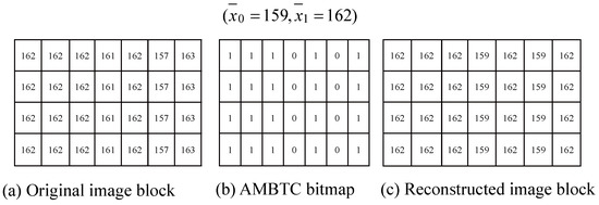
Figure 1.
Example of AMBTC compression with 4 × 7 block.
From the pixels in Figure 1a, finally the mean value AVG = 162, VAR = 1 are obtained. Any pixel values smaller than 162 are averaged and the results are rounded to the nearest integer to obtain . Similarly, is obtained. Subsequently, if pixels are smaller than 162 their corresponding bits are set as ‘0’ in the bitmap; otherwise, ‘1’. Finally, the corresponding AMBTC bitmap is derived, as shown in Figure 1b, and for a given original block shown in Figure 1a, its AMBTC-compressed trio is derived as (,, bitmap = 1110101 1110101 1110101 1110101). To generate the constructed image block, two-level quantizers AVG = 161 and VAR = 1 are used to derive L = 159 and H = 162 by Equation (2). Finally, ‘0’ and ‘1’ in the bitmap are replaced with L = 159 and H = 162, respectively, and the final reconstructed image is obtained, as shown in Figure 1c.
2.2. Lin et al.’s RDH Method
In 2015, Lin et al.’s RDH method [31] simply used the AVG and VAR generated by AMBTC to design their data hiding strategies instead of the two quantizers H and L. In their scheme, new two-level quantizers are defined in advance as AVG + VAR and AVG − VAR. Then, disjoint four disjoint cases are created by combining the bitmap and newly defined two-level quantizers. Finally, four hiding strategies for mapping to those four disjoint cases are demonstrated in Table 1.

Table 1.
Lin et al.’s four hiding strategies
With four disjoint data hiding cases and four hiding strategies, receivers can easily embed secret bits into embeddable blocks for more than two different pixels. Although Lin et al.’s hiding strategies slightly hamper the image quality of the steog-image, they remained disjoint pixel values in embeddable blocks after data embedding, and it is called as holding the same parity in this paper. Such property successfully guarantees the reversibility of Lin et al.’s RDH method and makes sure the hidden secret bits can be extracted according to Table 1 and Equation (2). Based on Lin et al.’s property which is holding the same parity after the data embedding, we explore the possibility of further enhancing the hiding capacity without reducing steog-image quality.
2.3. (7, 4) Hamming Code
Hamming codes [38] are a kind of linear error-correcting code, first invented by Richard Hamming in 1950. In this paper, (7, 4) Hamming code is applied to add three parities to four bits of secret data for data hiding with the advantage of detecting and correcting 1-error bit. In (7, 4) Hamming code, four data bits are encoded into seven bits C (also called ‘codeword’) by adding three parity bits via the generator matrix G of the Hamming code.
Next, codeword C is sent to the receiver. On the receiving side, the received seven-bit codeword R can be checked for errors by Equation (4) using the parity check matrix by a module of 2. It is noted that sy1, sy2 and sy3 are bits.
where, Equation (5) is below:
The computed result is called a ‘syndrome’. If the syndrome (sy1, sy2, sy3) is ‘000′, then R = C. If a single error bit occurs, the syndrome (sy1, sy2, sy3) will not equal ‘000′. Assume that codeword C = (1000110), the received codeword R’ has one error (e.g., R’ = (1100110), the calculated syndrome is ‘010′, which is identical to the second column of H0, and R is corrected by
where is the ith unit vector of length seven ( indicates a zero vector of length seven with a “1” located at the second position, = (0100000). By ignoring the last three parity bits, we can obtain the correct original data bits, i.e., d = (1000).
3. Improvement of Lin et al.’s Method
In Lin et al.’s RDH method, their data hiding strategies elegantly achieve two objectives: the property of holding the same parity is always maintained even after data embedding, and secret data can be concealed without causing complex computation. Unfortunately, the hiding capacity provided by their scheme is only 1 bpp. Based on holding the same parity property offered by Lin et al.’s method, we pursue a higher hiding capacity with (7, 4) Hamming code and propose a two-layer RDH for AMBTC-compressed images.
Our two-layer RDH scheme is divided into two parts: (1) a data embedding phase and (2) a data extraction and recovery phase. In the data embedding phase, Lin et al.’s four disjoint data hiding strategies are conducted in the first layer. Then, a new data hiding strategy based on (7, 4) Hamming code is conducted in the second layer, which follows the concept of (7, 4) Hamming code by modifying single bit to conceal three secret bits and extends Lin et al.’s four disjoint cases into eight by adding or subtracting 1 according to a matrix embedding with (7, 4) Hamming code. In the two-layer data hiding strategies, secret bit streams are divided into two parts—secret bits-1 and secret bits-2. During the data embedding phase, underflow or overflow may occur in the first and/or second layers. To avoid such problems, the following condition is defined in Equation (7). If only Equation (7) holds after data hiding, then the current block is determined to be embeddable; otherwise, it is un-embeddable.
In order to extract secret bits and completely recover an AMBTC-compressed image, in the first layer, if the unique number of pixels is less than 3 in a block, those blocks are determined as un-embeddable. In the second layer, either the number of embedded pixels is less than 6, or the number of different embedded pixels is 6, but the current processing block cannot be recovered as a lossless AMBTC-compressed block, the current processing block also is identified as un-embeddable one. The extraction phase also is divided into two: (1) when the number of different pixels is greater than or equal to 6, we use continuity feature (which means a set of different pixel values are continuous), the parity of modified pixel values, and the unique feature offered by our second-layer data hiding strategy (i.e., only one pixel value will be changed in a given row) to ensure that the hidden secrets Sb1 and Sb2 can be successfully extracted and the original two-level quantizers AVG and VAR can be stored; and (2) when the number of different pixels is 3 or 4, the parity of pixel values can also be used to extract hidden secrets Sb1 and restore the original two-level quantizers AVG and VAR. The proposed data embedding phase, along with examples of data embedding and irreversibility, are introduced in Section 3.1. Data extraction and recovery are explained in Section 3.2.
3.1. Data Embedding Phase
In the data embedding phase, the 512 × 512-sized grayscale image is first divided into k × 7 non-overlapping blocks. After AMBTC encoding, the trios (Bm_k × 7)ij, VARij and AVGij are generated for a given block (i, j), where k is 4, (Bm_k ×7)ij indicates a block’s bitmap, and (i, j) presents the block’s coordinates. Assume (Sb1_k × 7)ij is secret bits Sb1 and (Sb2_k × 3)ij is secret bits Sb2. Usually, k is set as 4 since (7, 4) Hamming code is adopted in the proposed method. As for the size of Sb1 is 4 × 7 = 28 bits and the size of Sb2 is 4 × 3 = 12 bits, this is because the hiding capacity for a given block with Lin et al.’s method in the first layer is the same as the block size and three secret bits can be concealed into seven bits as long as one single bit modification is required by adopting (7, 4) Hamming code in the second layer, respectively.
First, hide secret bits Sb1 (Sb1_k × 7)ij into bitmap (Bm_k × 7)ij according to the four disjoint cases defined in Lin et al.’s data hiding strategies [31]. Then, hide Sb2 (Sb2_k × 3)ij into bitmap (Bm_k × 7)ij using matrix embedding with (7, 4) Hamming code which is proposed in this paper. Finally, check the number of modified pixels to decide whether the stego block is reversible or not after two-layer data hiding. If the number of different pixels is less than 6, or the number of different embedded pixels is 6, but the current processing block cannot be recovered as a lossless AMBTC-compressed block, then we return the modified pixels to the previous state before performing embedding with (7, 4) Hamming code. The flowchart of the two-layer data embedding phase is depicted in Figure 2. The details of the procedure are as follows:
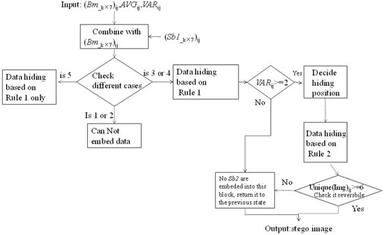
Figure 2.
Flowchart for embedding phase. Note: Rule 1 indicates Lin et al.’s data hiding strategy, it is also the hiding strategies adopted in the first layer; Rule 2 is the hiding strategies designed in the second layer.
Input: 4 × 7 block (B_k × 7)ij, its two-level quantizers VARij and AVGij, and two sets Sb1 and Sb2 of secret bits (Sb1_k × 7)ij and Sb2 (Sb2_k × 3)ij, respectively.
Output: Steog-image
Step 1: Combine secret bits Sb1 (Sb1_k × 7)ij and bitmap (Bm_k × 7)ij for the current processing (i, j) block to derive the modified pixel values according to data hiding rules listed in Table 1.
Step 2: Check the hidden pixels in a block. If the number of different hidden pixels is 1 or 2, the current block is un-embeddable and all modifications conducted in Step 1 must be undone. Otherwise, it is embeddable and we go to Step 3.
Step 3: If VAR of this block is greater than or equal to 2, we go to Step 4. Otherwise, no secret bits will be embedded.
Step 4: The secret bits Sb2 (Sb2_k × 3)ij are embedded into bitmap (Bm_k × 7)ij by using Equation (8) [38],
where m = Sb2_k × 3, x = Bm_k × 7, F(syndrome) = ek as mentioned in Section 2.3, then go to Step 5. As for Emd, which is bit assignment function and it can be used to generate the stego image y according to Mao defined in their work [39].
Step 5: Due to the second layer of data hiding with (7, 4) Hamming code, the bitmap needs to be changed. The corresponding position of each k row in block (B_k × 7)ij needs to be changed. The four hiding strategies designed for the second layer are presented in Table 2.
Table 2.
Four hiding strategies for the second layer
Step 6: If the number of modified pixel values S is equal to 5 for the current processing block, or if the number of modified pixel values S is equal to 6, but the block is determined as irreversible; which indicates that either continuity feature, the parity of modified pixel values is not holding or more than one pixel value has been changed after second-layer data embedding. All modifications made in Step 5 are cancelled and returned to the previous state.
Step 7: Proceed to the next block until all blocks have been completed. Finally, output the steog-image.
Example of Data Embedding Phase
An example is provided here to demonstrate the two-layer data hiding strategies shown in Figure 3. Assume the first secret stream Sb1 is {0001101; 0011111; 0110010; 0101001}, the 4 × 7 bitmap is {0001111; 0001111; 0000010; 0101001}, AVG = 50, VAR = 6 and the second secret stream Sb2 is {010; 101; 001; 000}.
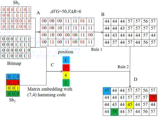
Figure 3.
Example of embedding phase. Note: Rule 1 indicates Lin et al.’s data hiding strategy, it is also the hiding strategies adopted in the first layer. Rule 2 is the hiding strategies designed in the second layer.
To conduct the first-layer data embedding, the first secret bit stream Sb1 is combined with a 4 × 7 bitmap. Note that the combination merges the first bit of Sb1 with that of the 4 × 7 bitmap as ‘00’. Follow the same concept, there are 28 pairs are derived. Take the first pair as ‘00’ for example, its pixel value should be modified as 44 (= 50 − 6) according to rule of Case00 defined in Table 1. Finally, modified pixels are generated as {44 44 44 57 57 56 57; 44 44 43 57 57 57 57; 44 43 43 44 44 57 44; 44 57 44 57 44 56 57} by adopting the modification rules defined in Table 1.
Once first-layer data embedding is completed, the second-layer data embedding begins. Noted that the number of different pixels is more than 3 in above example; therefore, all 4 × 7 blocks will be proceeded by conducting the second-layer data embedding to conceal secret bits of Sb2. For a given 4 × 7 block, the first seven bits are selected from the first row of the corresponding 4 × 7 bitmap as x as defined in Equation (8), and the first three bits are then selected from the second bit stream Sb2 to serve as m as defined in Equation (8). Finally, syndrome = (110)Tx is obtained, and its corresponding position is identified as the first row in H0. Take the first three bits of Sb2 as {010} for example. The first bit denoted ‘0’ of the first row of the 4 × 7 bitmap is determined to be changed according to Equation (8) and its corresponding modified pixel is equal to AVG − VAR after the first-layer data embedding. It can be categorized as Case00 as defined in Table 2. In other words, the corresponding pixel should be modified as 45(= AVG − VAR + 1 = 44 + 1). Following the same concept, the seventh position in the second row, the fourth position in the third row and the second position in the fourth row of Figure 3 are classified as Case11, Case00, and Case11, respectively. All modified pixels have been marked in blue, red, yellow, and green for different rows as shown in Figure 3 to provide a visual representation. Finally, the stego pixels after second-layer data embedding are {45 44 44 57 57 56 57; 44 44 43 57 57 57 58; 44 43 43 45 44 57 44; 44 58 44 57 44 56 57}. To ensure that reversibility can be guaranteed after data extraction, reversibility must be checked according to the rules defined in Step 6 of the data embedding phase.
Although the rules of reversibility are defined in Step 3 of data embedding phase, two cases of unreversible blocks are demonstrated below. These cases deem a block to be unreversible when it contains six or more different pixels. Here, blocks B1, B2, and B3 are used to demonstrate the application of our un-reversible rule in second-layer embedding.
Block B1, for instance, contains six pixels {4, 5, 6, 7, 23, 24} after second-layer data embedding. After checking the continuity feature and parity values of the modified pixels {4, 5, 6, 7, 23, 24}, we see two sublists—{4, 5, 6, 7} and {23, 24}. This is the “42” type, since, after second-layer data embedding, eight pixels at most can be found in the list of different pixels {(AVG – VAR − 2, AVG – VAR − 1, AVG − VAR, AVG − VAR + 1), (AVG + VAR, AVG + VAR − 1, AVG + VAR + 1, AVG + VAR + 2)}. By mapping the two sublists {4, 5, 6, 7} and {23, 24}, we can only conclude that AVG – VAR = 6. In other words, we cannot calculate the exact value of AVG and VAR for block B1. Therefore, block B1 is determined to be un-embeddable, and all modifications conducted in the second layer must be cancelled. The situation in block B3 is the same. As for block B2, two sublists can be found—{43, 44, 45} and {56, 57, 58}—but there are two possible candidates for the former: {AVG – VAR − 2, AVG – VAR − 1, AVG − VAR} and {AVG – VAR − 1, AVG − VAR, AVG – VAR + 1}. The same holds for the latter; therefore, it can be concluded that the modified pixel values have no parity property and block B2 is determined as unreversible one. Once the blocks listed in Table 3 are determined to be unreversible, all modifications conducted in the second-layer embedding will be undone and (Sb2_k × 3) will be embedded into the next block.
Table 3.
Unreversible example for cases where the number of different pixels inside a block is 6.
3.2. Extraction and Recovery Phase
Before the extraction and recovery phase, eight cases are concluded and guide the receiver to derive AVG and VAR according to the number of different modified pixels in a given block after two-layer data embedding. However, by mapping to the two-layer data embedding, two categories can be produced, depending on whether one-layer or two-layer data embedding has been conducted. If the numb of modified pixels is 3 or 4, only the first layer of the embedding phase has been performed and the current processing block only carries secret bits Sb1, so the original extraction phase defined in Lin et al.’s method [31] is applied. In contrast, if the number of modified different pixels is greater than or equal to 6, then secret bits Sb1 and Sb2 have been concealed in the current processing block. It is noted that the number different pixel values would not be equal to 5 since the second layer data hiding is terminated as mentioned in Step 6 in the data embedding phase to maintain the reversibility. To extract the hidden Sb2, our proposed extraction rules are listed below along with an overview of our extraction phase (Figure 4). As we mentioned earlier, S = 5 is not shown in Figure 4 because our embedding operation of the second layer is terminated if the number of different values is equal to 5.
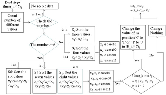
Figure 4.
Flowchart of extraction and recovery phase. Note: S indicates the number of different pixel values.
Input: steog-image (Imag_k × 7)ij
Output: secret bits Sb1, secret bits Sb2, AVG and VAR
Step 1: Count the amount of modified values denoted as S, and S = {1, 2, 3, 4, 6, 7, 8} inside the current processing stego-block. If S is 1 or 2, then the stego-block has carried no secret. Otherwise, go to Step 2. It is noted that S would not equal to 5 since the embedding operation in the second layer data hiding is not proceeded when the number of different pixel values is equal to 5.
Step 2: If the different pixel values S is less than 6, then go to Step 3. Otherwise, go to Step 5.
Step 3: If S = 3, follow the flowchart for the extraction phase, shown in Figure 5. Sort the three different values as x1 <x2 <x3, and compare (x3 - x2) and ( x2 – x1). If x3 – x2 > x2 – x1, and , then check the parity property among x3, x2; if Parity(x3, x2) = 0, then x3 and x2 are either both even or odd, and it can be concluded that . Otherwise, . If , then . and .. Check the parity property between x2 and x1. If Parity(x1, x2)=0, then x1 and x2 are either both even or both odd, and . Otherwise, . Since we know three pixels, the fourth can be calculated according to Table 1. Then, from Table 1, we can easily extract Sb1 and calculate AVG and VAR.
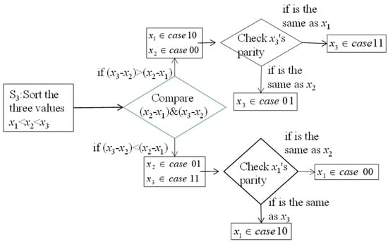
Figure 5.
Flowchart of extraction phase when S = 3. Note: S indicates the number of different pixel values.
Step 4: If S = 4, we sort the different pixel values as and directly calculate AVG and VAR by the formula . According to Table 1, we can extract Sb1.
Step 5: If S = 6, go to Step 6. If S = 7, go to Step 7. Otherwise, go to Step 8.
Step 6: If S = 6, following the flowchart for the extraction phase in Figure 6, sort the different pixel values as , which can be divided into three Types: 42, 24 and 33. Since Type 42 has the same situation as Type 24, we illustrate Types 42 and 33 as Figure 6 and Figure 7, respectively.
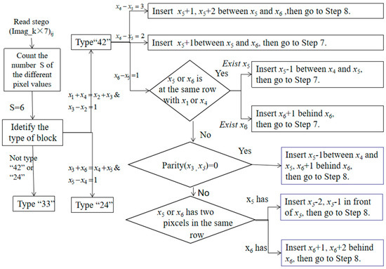
Figure 6.
Flowchart of extraction phase when S = 6. Type 42, Note: S indicates the number of different pixel values.
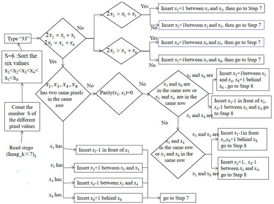
Figure 7.
Flowchart of extraction phase when S = 6. Type 33, Note: S indicates the number of different pixel values.
Step 7: If S = 7, the flowchart for extraction is shown in Figure 8. Sort the different pixel values as , which can be divided into Types 43 and 34, where “43” means that the first four values are less than AVG, and the last three are greater than AVG. Type 34 is the opposite, so we simply illustrate the former Type 43 in Figure 8. If x1 + x4 = x2 + x5 and x3 − x2 = 1, then the leftmost four pixels are continuous natural numbers. It is noted that x3=AVG-VAR. In this case, we simply need to check the rightmost four pixels: (1) if 2x6 = x5 + x7, then the rightmost three pixels are continuous natural numbers. Then check the parity of x3 and x5. If Parity(x3,x5) = 0, then it can be concluded that x5 = AVG + VAR. So insert x5-1 between x4 and x5, and go to Step 8. Otherwise, it can be concluded that x6 = AVG + VAR. In this case, insert x7+1 behind x7, and go to Step 8; (2) if 2x6 > x5 + x7, then the rightmost three pixels are not continuous natural numbers, so x7 is closer to x6 than to x5, and x5 and x6 are not continuous natural numbers; therefore, insert x5 + 1 between x5 and x6, and go to Step 8; (3) if 2x6 < x5 + x7, we do the same as in (2), then insert x6 + 1 between x6 and x7, and go to Step 8.
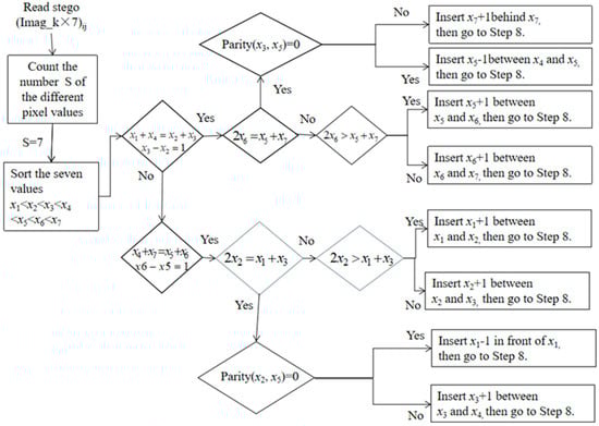
Figure 8.
Flowchart of extraction phase when S = 7. Type 43, Note: S indicates the number of different pixel values.
Step 8: If S = 8, sort the eight different values as , and we can conclude that , , . Next, check whether pixels located in the kth column and mth row in the block are equal to either x1, x4, x5, or x8. If so, then flip the corresponding bit value of the bitmap. Otherwise, no pixels have been flipped in any row. Finally, multiply H0T with each block according to Equation (9) to extract the hidden secret (Sb2_k × 3)ij.
where m’ is extracting Sb2, and y is the changed value of (Bm_k × 7)ij.
m’ = H0 syndrome
Example of Data Extraction and Recovery Phase
Here, a block containing six different pixel values (Figure 9), is used to demonstrate how our proposed data extraction and recovery works. Assume a 4 × 7-sized block {45 44 44 57 57 56 57; 44 44 43 57 57 57 58; 44 43 43 45 44 57 44; 44 58 44 57 44 56 57} as below. According to the flowchart of the extraction phase in Figure 4, the number of different pixel values in a 4 × 7 block is 6. Sorting these six different values yields a sorted value stream of {43, 44, 45, 56, 57, 58}. In this stream, there are three continuous values on the left and three on the right. Therefore, the block shown in Figure 10 is Type 33, because it satisfies 2x2 = x1 + x5 and 2x5 = x4 + x6. According to the flowchart of the extraction phase shown in Figure 8, two pixels have the same values as x1 = 43, and they are located in the same row (marked in red). This means that it cannot be the changed pixel, so insert x1 – 1 = 42 in front of x1. Here, a new sorted value stream—denoted as {42, 43, 44, 45, 56, 57, 58}—is obtained and belongs to Type 43.
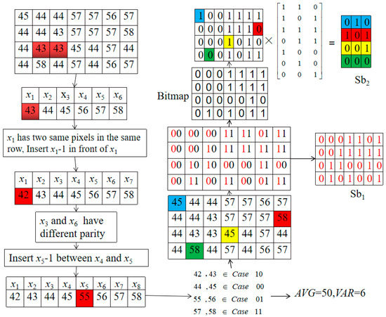
Figure 9.
Example of extraction and recovery phase.
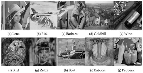
Figure 10.
Ten test grayscale images: (a) Lena, (b) F16, (c) Barbara, (d) Goldhill, (e) Wine, (f) Bird, (g) Zelda, (h) Boat, (i) Baboon, (j) Peppers.
Since this value stream has seven different pixel values, it belongs to Type 43 and satisfies 2x6 = x5 + x7, so the parity of x3 and x6 is checked. In this case, x3 = 44 and x6 = 56, both of which are even, so Parity (x4, x6) = 0; therefore, x5 − 1 = 55 is inserted between x4 and x5, and a new sorted value stream is obtained—{42, 43, 44, 45, 55, 56, 57, 58}. Eventually, we can see that {42, 43} belongs to Case 10; {44, 45} belongs to Case 00; {55 56} belongs to Case 01; and {57, 58} belongs to Case 11, based on Step 8 of the extraction and recovery algorithm shown in Figure 4. Finally, the original two quantizer levels can be easily derived from AVG = (44 + 56)/2 = 50 and VAR = (56 − 44)/2 = 6, respectively. Based on the rules listed in Table 1, two bits can be derived from a pixel, and a bit block can be transformed from the pixel block. The former bits (marked red in Figure 10) can be collected to obtain the hidden secret bits Sb1. The remaining bits are collected to derive the bitmap. From 45, 58, 45, and 58—colored blue, red, yellow, and green in the pixel block, respectively—we know that the values of the bitmap need to be changed in the corresponding positions. Thus, we change the original bitmap value of the corresponding position to its opposite value. And by multiplying , we obtain the secret bits Sb2.
4. Experiment Results and Discussion
This section presents experimental results to demonstrate how our proposed method outperforms existing methods. All experiments were implemented in MATLAB R2014b on a PC with Intel® Core (TM) i7-8750H CPU @2.20 GHz, 16 GB RAM. Ten standard grayscale images of 512 × 512 resolution—Lena, F16, Barbara, Gold hill, Wine, Bird, Zelda, Boat, Baboon, and Peppers shown in Figure 10—were drawn from the USC-SIPI data [40].
Three criteria are utilized to measure the performance of the proposed method—peak signal-to-noise ratio (PSNR), hiding capacity (HC) and embedding efficiency rate (ER). As we know that PSNR is used to estimate the visual quality of an AMBTC-compressed image, which is defined in Equation (10), where xi,j and x’i,j indicates the pixel value of the coordinate (i, j) of the original image and of the AMBTC-compressed steog-image, respectively. HT and WH represent the height and width of the image, respectively.
To examine the performance of different types of RDH schemes, we utilize the embedding efficient rate (ER) by Equation (11)
where HC and stego_size represent the total of embedded secret bits and the size of stego bitstream codes, respectively. An embedding method with higher ER indicates that it offers a larger payload for stego bitstream codes.
4.1. Performance of Proposed Method
In this subsection, we demonstrate the performance of our improved method under different partitions. Our improved method can restore the original two quantizer levels AVG and VAR from the steog-image, apart from special cases when the number of different pixels in a block is 6, but the block is determined to be irreversible after data embedding. Such unique cases are presented in Table 4 under different partitions.
Table 4.
Number of irreversible blocks when a block contains six different pixels.
Here, we can see that even in a 4 × 7 partition, only one case is found in Lena, Barbara, and Zelda, respectively. It is concluded that these irreversible blocks do not affect the hiding capacity of our improved method. Therefore, no extra information is required to record these irreversible data. It is simple to ignore or cancel the modification that has been done once the block is determined to be irreversible. Through this arrangement, the reversibility of our improved method is maintained while achieving a high hiding capacity.
The performance of our proposed method with different block sizes is shown in Table 5. Although the first-layer hiding strategy is the same as Lin et al.’s method [9], we changed the partition size in our improved method from 4 × 4 to 4 × 7 or 8 × 7, to extend it to the second-layer data hiding operations. Therefore, we can see that the PSNR of the first layer is slightly lower with our improved method than that achieved by the original AMBTC. With our proposed method, the ‘Bird’ and ‘Baboon’ images, which are relatively complex, have a lower PSNR, but a higher capacity in 4 × 7 and 8 × 7 partitions. This is because they offer more blocks that contain six or more different pixel values in a block, as compared with smoother images. The hiding capacity of ‘Wine’, for example, can be increased from 343,096 to 35,072 bits when a block size is changed from 4 × 7 to 8 × 7. As for the remaining images, the general increased number of secret bits remains around 10,000 bits. This is because in the larger partition, with fewer smooth blocks, there are more numerous embeddable blocks. If we explore the relationship between the hiding capacity and PNSR with our proposed method, we can see that that the highest hiding capacity with our proposed two-layer data hiding strategies is up to 368,348 bits with ’Baboon’ under block size 4 × 7 while maintaining PSNR as 25.6 dB which is lower 0.5 dB than the original BTC. This is because we adopt the (7, 4) Hamming code to achieve the reversible data hiding in the second layer. With the concept of (7, 4) Hamming code, three secret bits can be embedded into the embeddable stego blocks after the first layer data hiding at the cost of single bit modification. Certainly, to maintain all modifications caused in the second layer can be successfully restored in the recovery phase, many rules are designed to decide whether the stego blocks after the first layer can be proceeded in the second layer data hiding or not. However, in Table 5 we will find such judgements do not cause too much computation cost but make sure the reversibility of our proposed method.
Table 5.
Performance of proposed method with different block sizes (unit: dB)
Because the 4 × 7 and 8 × 7 partitions are not generally adopted by conventional AMBTC, we slightly modified our partition to n × n in order to increase applicability. Corresponding data is presented in Table 5. Generally speaking, six different pixels can be found inside a 4 × 4 block when adopting our proposed (7, 4) Hamming code-based data hiding strategy. This is because in a 4 × 4 block, two sets can be obtained, each of which has 7 bits derived from its corresponding bitmap. The core concept of (7, 4) Hamming code is that only one bit is modified after data embedding. Under such circumstances, our improved method would not retain enough information to conclude the original two quantizer levels VAR and AVG in the extraction and recovery phase. Therefore, our embedding strategy must be slightly modified as follows.
First, all n × n embeddable blocks are expanded into 1 × n2 and linked together to form a (1 × n)2× N table, where N denotes the number of embeddable blocks. 1 × 7 continuous bits are selected from the bitmap to conduct our proposed (7, 4) Hamming code-based data hiding strategy. The only modification is as follows: when the mth bit is determined to be changed after the (7,4) Hamming code-based data hiding strategy at the first 1 × 7 data set, the corresponding pixel of mth is then modified instead of its corresponding bit value on the bitmap. To embed the next secret bit, the second 1 × 7 data set begins from the (m + 1)th. If the second data set does not cause any modification, then the next 1 × 7 data set begins from the next seven bits. Certainly, every 4 × 4 data set needs to be checked for reversibility after data embedding. All reversibility rules are the same as above, except each row can carry more than one single secret bit. During data extraction, the corresponding bit in the bitmap is changed from ‘1’ to ‘0,’ or vice versa, when the first pixel value to differ from previous ones is determined. Let us assume that the first pixel value that differs is located at the mth. For the remaining data extraction, the next data set begins from the (m + 1)th. In the modified (7, 4) Hamming code-based data hiding strategy, since the construction is defined in our initial data hiding strategy: each row that hides only a single secret bit has been omitted; thus, hiding capacity increases. The experimental data of embedding capacity with our modified (7, 4) Hamming code-based data hiding strategy is shown in Table 6. Notably, the hiding capacity for 8 × 8 is significantly higher than that for 8 × 7, as shown in Table 5. The hiding capacity offered by 4 × 4 is lower than that of 4 × 7, but the corresponding PSNRs are significantly improved.
Table 6.
Comparison of six methods
4.2. Performance Comparison with Related Studies
In this subsection, to further demonstrate our method’s contribution, we compare its improved performance with five existing works, including Chang et al. [27], Lin et al. [31], Pan et al. [32], and Hong et al. [27,28]. Chang et al. and Hong et al.’s methods are based on Sun et al. [20], while Lin et al. and Pan et al. use four hiding strategies to conceal a secret message into a bitmap. Three criteria—PSNR, HC, and ER—are used to demonstrate related data with different methods. Results of the comparison are shown in Table 6.
As shown in Table 6, the PSNR of our improved method is quite close to that of Lin et al.’s scheme, but our method has the highest HC than other existing methods. The significant difference between the proposed method and the others is that richly textured images will offer a higher hiding capacity with our improved method; i.e., ‘Baboon’ can carry 352,795 bits, more than doubling the capacity of Chang et al.’s method (151,439 bits). Our proposed method offers the highest HC than other methods because our method extends Lin’s four hiding strategies and uses two-layer data embedding strategies. On the ER side, the result is slightly inferior to Chang et al.’s method, but compared with other methods, our ER still outperforms other methods.
Except the performance on hiding capacity, PSNR and ER, computation complexity is also the other criterion to evaluate the performance of the RDH scheme. In Table 7, the computation operations adopted in data embedding and data extracting phases are listed. We can find schemes of Lin et al. [31] and Pan et al. [32] used either table lookup or reference matrix checking to conduct data embedding and data extracting phases, respectively. Therefore, the computation complexity of both of two schemes are the lowest. As for our proposed method, there are two layers of data hiding and data extracting. The first layer data hiding operation of our proposed method simply inherits from Lin et al.’s scheme [31] but the second layer data hiding operation is (7, 4) Hamming coding. In other words, the second layer data hiding of our proposed method is matrix coding operation. In the contrast, only table lookup operation is required for both first layer and the second layer of data extracting operations. Therefore, the computation complexity of our proposed method is relatively higher than schemes of Lin et al.’s [31] and Pan et al.’s [32].
Table 7.
Comparison of six methods on computation operations
Hong et al.’s scheme [28] needs three kinds operations such as calculating prediction error, table lookup, and concatenation to embed secret bits. In Chang et al.’s scheme [27], they needed to perform XOR operation when embedding secret bits. Therefore, these two schemes require relatively higher computation complexity than Lin et al.’s scheme [31], Pan et al.’s scheme [32] and our proposed method. As for Hong et al.’s scheme [29], their computation complexity is the highest among six schemes because they needed to classify blocks into complex and smooth blocks first. Then, for smooth blocks, minimal distortion computation and reference matrix checking are conducted for carrying secret bits. For complex blocks, flipping operation is required to conceal secret bits.
Comparing performance on hiding capacity, PSNR, ER, and computation operations listed in Table 6 and Table 7, we found the computation complexity of our proposed method is not the lowest, and it is relatively higher than that of schemes of Lin et al. [31] and Pan et al. [32]; however, the hiding capacity of our proposed method is 1.15 times of that of two schemes in the worst case. In other words, we can conclude our proposed method successfully significantly enhance the hiding capacity while maintaining acceptable computation complexity.
5. Conclusions
In this paper, an effective two-layer data hiding method was proposed for AMBTC-compressed images using (7, 4) Hamming code. In the first layer, four disjoint sets using different combinations of AVG and VAR are derived according to the combination of the secret bits and a bitmap, following Lin et al.’s method. In the second layer, these four disjoint sets are extended to eight by adding or subtracting 1 according to a matrix embedded with (7, 4) Hamming code. In the data extraction and recovery phase, continuity feature, parity of pixels, and the unique number of changed pixel in the same row are used to restore AVG and VAR. The experiments demonstrate that our proposed method has the highest HC among six representative BTC or AMBTC-family based RDH schemes. Moreover, the computation complexity of our proposed method is next to schemes of Lin et al.’s [31] and Pan et al.’s [32] since matrix coding is required in the second layer data hiding but only table lookup operation is required for the second layer data extracting. We can conclude our proposed method is suitable for real-time applications. However, considering attacks supported by deep learning [41] or other technologies [42] may cause the hidden security unsecure or the forged stego image. In the future, we hope to explore ways of further enhancing the security of hidden data or identifying the valid stego image while maintaining high HC and low computation complexity, so that our proposed method can be more practical for various applications.
Author Contributions
Conceptualization, C.-C.L. and C.-C.C.; Methodology, J.L.; Software, J.L.; Writing—original draft preparation, J.L.; Writing—review and editing, C.-C.L. All authors have read and agreed to the published version of the manuscript.
Funding
This research was funded by MOST 109-2410-H-167-014.
Conflicts of Interest
The authors declare no conflict of interest.
References
- Lin, C.C.; Chang, C.C.; Wang, Z.M. Reversible data hiding scheme using adaptive block truncation coding based on an edge-based quantization approach. Symmetry 2019, 11, 765. [Google Scholar] [CrossRef]
- Peticolas, F.; Anderson, R.; Kuhn, M. Information hiding—A survey. Proc. IEEE 1999, 87, 1062–1068. [Google Scholar] [CrossRef]
- Hong, W.; Chen, T.S.; Chen, J. Reversible data hiding using delaunay triangulation and selective embedment. Inf. Sci. 2015, 308, 140–154. [Google Scholar] [CrossRef]
- Chan, C.K.; Cheng, L.M. Hiding data in images by simple LSB substitution. Pattern Recognit. 2004, 37, 469–474. [Google Scholar] [CrossRef]
- Ni, Z.C.; Shi, Y.Q.; Ansari, N.W.; Su, W. Reversible data hiding. IEEE Trans. Circuits Syst. Video Technol. 2006, 16, 354–362. [Google Scholar] [CrossRef]
- Lin, C.C.; Tai, W.L.; Chang, C.C. Multilevel reversible data hiding based on histogram modification of difference images. Pattern Recognit. 2008, 41, 3582–3591. [Google Scholar] [CrossRef]
- Zhang, D.Z.; Panand, Z.; Li, H. A contour-based semi-fragile image watermarking algorithm in DWT domain. In Proceedings of the Second International Workshop on Education Technology and Computer Science, Wuhan, China, 6–7 March 2010; pp. 228–231. [Google Scholar]
- Wu, X.; Sun, W. Robust copyright protection scheme for digital images using overlapping DCT and SVD. Appl. Soft Comput. 2013, 13, 1170–1182. [Google Scholar] [CrossRef]
- Gray, R.M. Vector quantization. IEEE Assp. Mag. 1984, 1, 4–29. [Google Scholar] [CrossRef]
- Kim, T. Side match and overlap match vector quantizers for images. IEEE Trans. Image Process. 1992, 1, 170–185. [Google Scholar] [CrossRef]
- Delp, E.J.; Mitchell, O.R. Image compression using block truncation coding. IEEE Trans. Commun. 1979, 27, 1335–1342. [Google Scholar] [CrossRef]
- Wang, K.; Lu, Z.M.; Hu, Y.J. A high capacity lossless data hiding scheme for JPEG images. J. Syst. Softw. 2013, 86, 1965–1975. [Google Scholar] [CrossRef]
- Lema, M.; Mitchell, O. Absolute moment block truncation coding and its application to color images. IEEE Trans. Commun. 1984, 32, 1148–1157. [Google Scholar] [CrossRef]
- Kumar, R.; Kim, D.S.; Jung, K.H. Enhanced AMBTC based data hiding method using hamming distance and pixel value differencing. J. Inf. Secur. Appl. 2019, 47, 94–103. [Google Scholar] [CrossRef]
- Li, C.H.; Lu, Z.M.; Su, Y.X. Reversible data hiding for BTC-compressed images based on bitplane flipping and histogram shifting of mean tables. Inf. Technol. J. 2011, 10, 1421–1426. [Google Scholar] [CrossRef][Green Version]
- Lin, C.C.; Liu, X.L. A reversible data hiding scheme for block truncation compression based on histogram modification. In Proceedings of the Sixth International Conference Genetic and Evolutionary Computing (ICGEC), Kitakyushu, Japan, 25–28 August 2012; pp. 157–160. [Google Scholar]
- Chang, C.I.; Hu, C.Y.; Chen, L.W.; Lu, C.C. High capacity reversible data hiding scheme based on residual histogram shifting for block truncation coding. Signal Process. 2015, 108, 376–388. [Google Scholar] [CrossRef]
- Li, F.; Bharanitharan, K.; Chang, C.C.; Mao, Q. Bi-stretch reversible data hiding algorithm for absolute moment block truncation coding compressed images. Multimed. Tools Appl. 2016, 75, 16153–16171. [Google Scholar] [CrossRef]
- Chuang, J.C.; Chang, C.C. Using a simple and fast image compression algorithm to hide secret information. Int. J. Comput. Appl. 2006, 28, 735–743. [Google Scholar]
- Ou, D.; Sun, W. High payload image steganography with minimum distortion based on absolute moment block truncation coding. Multimed. Tools Appl. 2015, 74, 9117–9139. [Google Scholar] [CrossRef]
- Huang, Y.H.; Chang, C.C.; Chen, Y.H. Hybrid secret hiding schemes based on absolute moment block truncation coding. Multimed. Tools Appl. 2017, 76, 6159–6174. [Google Scholar] [CrossRef]
- Chen, Y.Y.; Chi, K.Y. Cloud image watermarking: High quality data hiding and blind decoding scheme based on block truncation coding. Multimed. Syst. 2019, 25, 1–13. [Google Scholar] [CrossRef]
- Wang, K.; Hu, Y.; Lu, Z.M. Reversible data hiding for block truncation coding compressed images based on prediction-error expansion. In Proceedings of the Eighth International Conference on Intelligent Information Hiding and Multimedia Signal Processing, Piraeus-Athens, Greece, 18–20 July 2012; pp. 317–320. [Google Scholar]
- Sun, W.; Lu, Z.M.; Wen, Y.C.; Yu, F.X.; Shen, R.J. High performance reversible data hiding for block truncation coding compressed images. Signal Image Video Process. 2013, 7, 297–306. [Google Scholar] [CrossRef]
- Hong, W.; Ma, Y.B.; Wu, H.C. An efficient reversible data hiding method for AMBTC compressed images. Multimed. Tools Appl. 2017, 76, 5441–5460. [Google Scholar] [CrossRef]
- Tsai, Y.Y.; Chan, C.S.; Liu, C.L.; Su, B.R. A reversible steganographic algorithm for BTC-compressed images based on difference expansion and median edge detector. Image Sci. J. 2014, 62, 48–55. [Google Scholar] [CrossRef]
- Chang, C.C.; Chen, T.S.; Wang, Y.K.; Liu, Y.J. A reversible data hiding scheme based on absolute moment block truncation coding compression using exclusive OR operator. Multimed. Tools Appl. 2018, 77, 9039–9053. [Google Scholar] [CrossRef]
- Hong, W.; Zhou, X.Y.; Weng, S.W. Joint adaptive coding and reversible data hiding for AMBTC compressed images. Symmetry 2018, 10, 254. [Google Scholar] [CrossRef]
- Hong, W. Efficient data hiding based on block truncation coding using pixel pair matching technique. Symmetry 2018, 10, 36. [Google Scholar] [CrossRef]
- Sun, S.; Yin, Z.; Tang, J.; Luo, B. Improved reversible data hiding scheme based on AMBTC compression technique. In International Conference on Industrial IoT Technologies and Applications; Springer: Cham, Switzerland, 2017; pp. 111–118. [Google Scholar]
- Lin, C.C.; Liu, X.L.; Tai, W.L.; Yuan, S.M. A novel reversible data hiding scheme based on AMBTC compression technique. Multimed. Tools Appl. 2015, 74, 3823–3842. [Google Scholar] [CrossRef]
- Pan, J.; Li, W.; Lin, C.C. Novel reversible data hiding scheme for AMBTC-compressed Images by reference matrix. In Proceedings of the Multidisciplinary Social Networks Research, Kaohsiung, Taiwan, 13–14 September 2014; pp. 427–436. [Google Scholar]
- Zhang, Y.; Guo, S.Z.; Lu, Z.M.; Luo, H. Reversible data hiding for BTC-compressed images based on lossless coding of mean tables. IEICE Trans. Commun. 2013, 96, 624–631. [Google Scholar] [CrossRef]
- Huynh, N.T.; Bharanitharan, K.; Chang, C.C.; Liu, Y.J. Minima-maxima preserving data hiding algorithm for absolute moment block truncation coding compressed images. Multimed. Tools Appl. 2018, 77, 5767–5783. [Google Scholar] [CrossRef]
- Chang, C.C.; Kieu, T.D.; Chou, Y. A high payload steganographic scheme based on (7, 4) hamming Code for digital images. In Proceedings of the International Symposium on Electronic Commerce and Security, Guangzhou, China, 3–5 August 2008; pp. 16–21. [Google Scholar] [CrossRef]
- Cao, Z.; Yin, Z.; Hu, H.; Gao, X.; Wang, L. High capacity data hiding scheme based on (7, 4) hamming code. SpringerPlus 2016, 5, 175. [Google Scholar] [CrossRef]
- Bai, J.; Chang, C.C. A high payload steganographic scheme for compressed images with hamming code. Int. J. Netw. Secur. 2016, 18, 1122–1129. [Google Scholar]
- Hamming, R.W. Error detecting and error correcting codes. Bell Syst. Tech. J. 1950, 29, 147–160. [Google Scholar] [CrossRef]
- Mao, Q. A fast algorithm for matrix embedding steganography. Digit. Signal Process. 2014, 25, 248–254. [Google Scholar] [CrossRef]
- The USC-SIPI Image Database. Available online: http://sipi.usc.edu/database (accessed on 20 January 2020).
- Akhtar, N.; Mian, A. Threat of adversarial attacks on deep learning in computer vision: A survey. IEEE Access 2018, 6, 14410–14430. [Google Scholar] [CrossRef]
- Chakraborty, T.; Jajodia, S.; Katz, J.; Picariello, A.; Sperli, G.; Subrahmanian, V.S. FORGE: A fake online repository generation engine for cyber deception. IEEE Trans. Dependable Secur. Comput. 2019. [Google Scholar] [CrossRef]
Publisher’s Note: MDPI stays neutral with regard to jurisdictional claims in published maps and institutional affiliations. |
© 2021 by the authors. Licensee MDPI, Basel, Switzerland. This article is an open access article distributed under the terms and conditions of the Creative Commons Attribution (CC BY) license (http://creativecommons.org/licenses/by/4.0/).