Design of Cut Off-Frequency Fixing Filters by Error Compensation of MAXFLAT FIR Filters

Abstract

Maximally-flat (MAXFLAT) finite impulse response (FIR) filters often face a problem of the cutoff-frequency error due to approximation of the desired frequency response by some closed-form solution. So far, there have been plenty of efforts to design such a filter with an arbitrarily specified cut off-frequency, but this filter type requires extensive computation and is not MAXFLAT anymore. Thus, a computationally efficient and effective design is needed for highly accurate filters with desired frequency characteristics. This paper describes a new method for designing cutoff-frequency-fixing FIR filters through the cutoff-frequency error compensation of MAXFLAT FIR filters. The proposed method provides a closed-form Chebyshev polynomial containing a cutoff-error compensation function, which can characterize the “cutoff-error-free” filters in terms of the degree of flatness for a given order of filter and cut off-frequency. This method also allows a computationally efficient and accurate formula to directly determine the degree of flatness, so that this filter type has a flat magnitude characteristic both in the passband and the stopband. The remarkable effectiveness of the proposed method in design efficiency and accuracy is clearly demonstrated through various examples, indicating that the cutoff-fixing filters exhibit amplitude distortion error of less than 10⁻¹⁴ and no cut off-frequency error. This new approach is shown to provide significant advantages over the previous works in design flexibility and accuracy.

1. Introduction

The theory, design, and application of a finite impulse response (FIR) filter with mathematical analysis have been widely studied [1,2,3,4,5,6,7,8,9,10,11,12,13,14,15,16,17,18,19,20,21,22,23]. Among them, especially, maximally-flat (MAXFLAT) FIR filters, which are known for their design simplicity, accuracy, and high stopband attenuation, have an important role in some applications, such as waveform transmission and audio/image processing [3,4,5,6,7,8,9,10,11,12,13,14]. The basic idea for the design of MAXFLAT FIR filters is based on the well-known closed-form transform function and is realized due to its closed-form polynomial [7,8,9,15,16,17,18]. However, previous MAXFLAT FIR filter designs involve approximation of the desired frequency response by some closed-form polynomial, like a Hermite Interpolation [15], Miller’s conformal mapping [16], Bernstein polynomial [10,17], Fahmy’s Integral method [18], or Krawtchouk polynomial [19], which is then mapped to the filter function by certain transformations. The MAXFLAT FIR filter by any closed-form polynomial does not have any independent (“free”) parameters. This is due to the fact that the maximum possible number of zeros at $z=\pm 1$ is imposed, which leaves no degree of freedom, and, thus, no independent parameters. Thus, there is no direct control over the frequency response to obtain such a filter with a prescribed specified cut off-frequency. For that reason, the magnitude response of this filter type never passes through the desired cut off-frequency [19,20,21,22]. In order to overcome such a difficulty, there have been many efforts for comprising independent parameters in a closed-form function and, then, frequency response by (modified) closed-form function is controllable by these parameters. FIR filters using such a closed-form function including controllable parameters are no longer MAXFLAT, and, thus, various design methods have been published recently to obtain a best frequency response [7,8,9,10,11,12,13,14,23]. Jeon et al. have reported a closed-form least error gain method [23] for the design of FIR filters with both a flat magnitude and exact cut off-frequency. However, this method has the disadvantage of requiring a lot of computation processing for estimating the order of flatness, so that the error frequency function is closest to a zero gain at all frequencies [23]. It also sometimes has the frequency response distortion by wrongly determining the order of flatness. Huang et al. have proposed a closed-form weighted least square design to obtain FIR filters with exact cut off-frequency. However, this method has the disadvantage of providing non-negligible amplitude distortions of more than 4.2% by the Gibbs effect despite allowing a large amount of computation for estimating a convolution window [7,8]. Tseng and Lee introduced a closed-form design by mapping three discrete transforms, but there is a serious problem, such that filter cutoff-frequency error rapidly increases with growing cut off-frequency [9]. Recently, Roy et al. have reported Chebyshev closed-form FIR filters using a Bernstein polynomial [10]. They can reduce the filter design complexity by using a specific threshold value, but non-negligible amplitude distortions are in the stopband and passband. Hence, a computationally efficient design is needed for highly accurate filters with desired frequency characteristics, i.e., magnitude response exactly passes through prescribed, specified cutoff-frequency and is maximally flat in both the passband and the stopband.

The objective of this paper is to present a new method for the design of cut off-frequency fixing filters using a “cut off-error-free” polynomial function. For this purpose, a frequency-response error compensation function between the desired and actual frequency responses is derived through the generalization of the three closed-form polynomials [10,15,16,17] into a Chebyshev polynomial form. The proposed method provides a closed-form Chebyshev polynomial to characterize this filter type in terms of the degree of flatness for a given order of filter and cut off-frequency. Then, the magnitude response passes exactly through the prescribed specified cut off-frequency, and the filter also has independent (“free”) parameters that permit direct control over the frequency response, i.e., there is a tradeoff between the transition bandwidth and the magnitude flatness [24]. Finally, to determine the degree of flatness, so that a (cut off-frequency fixing) filter has a flat magnitude response characteristic for a given order of filter and cut off-frequency, a computationally efficient and accurate formula is derived from the cut off error compensation function.

This paper is organized as follows. In Section 2, we propose a closed-form error function for the cut off-error compensation of MAXFLAT FIR filters and introduce a closed-form Chebyshev polynomial to design cut off-frequency fixing filters. In Section 3, through the analysis of this error compensation function, we provide an exact and direct expression to choose a cutoff-frequency fixing FIR filter with a desired frequency response. Design examples that demonstrate the power of the new technique are shown. Conclusions are drawn in Section 4.

2. Closed-Form Chebyshev Polynomial for Cutoff-Frequency Fixing Filter Design

The transfer function $H\left(z\right)$ of a symmetric linear-phase FIR filter with the impulse response $h_n$ of order $2N$ is written as:

$$H\left(z\right)={\displaystyle \sum }_{n=0}^{2N}{h}_n{z}^{-n}=z^{-N}\left\{h_N+{\displaystyle \sum }_{n=1}^N{h}_{N-n}{T}_n\left(\omega \right)\right\}$$

(1)

where $T_n\left(\omega \right)$ is the Chebyshev polynomial of the first kind of degree n, and the independent transformed variable $w$ [25] is related to the digital domain by:

$$w=\frac{1}{2}\left(z+z^{-1}\right){|}_{z=e^{j\omega }}=cos\omega$$

(2)

confined to the interval [−1, 1]. The frequency response $H\left(e^{j\omega }\right)$ of the filter can be expressed as:

$$H\left(e^{j\omega }\right)=e^{-jN\omega }Q\left(cos\omega \right)=z^{-N}Q\left(w\right){|}_{z=e^{j\omega }}$$

(3)

by using the zero-phase transfer function $Q\left(w\right),$ which represents a polynomial of the real variable $w=cos\omega$, $\left(0\le \omega \le \pi \right)$. Then, the filter can be said to be lowpass and MAXFALT if $Q\left(cos\omega \right)$ has the following properties:

$${Q\left(cos\omega \right)|}_{\omega =0}=1$$

(4)

$${\frac{{\partial }^{v}Q\left(cos\omega \right)}{\partial {\omega }^v}|}_{\omega =0}=0,v=1,2,\dots ,2\left(N-K\right)+1$$

(5)

$${\frac{{\partial }^{v}Q\left(cos\omega \right)}{\partial {\omega }^v}|}_{\omega =\pi }=0,v=0,1,2,\dots ,2K-1$$

(6)

where N − K and K represent orders of flatness at $\omega =0$ and $\omega =\pi$, respectively. It is shown, based on the results of [10,15,16,17], that such a lowpass function can be accomplished by using one of the closed-form polynomials, namely, Hermite Interpolation polynomial [15], Miller’s conformal mapping function [16], and Bernstein polynomial [10,17], which are expressed, respectively, as:

$$P_{N,K}\left(x\right)={(1-x)}^K{\displaystyle \sum }_{i=0}^{N-K}\left(\begin{array}{c}K+i-1\\ i\end{array}\right)x^i,0\le x\le 1$$

(7)

$$H_{N,K}\left(j\mathsf{\Omega }\right)=\frac{1}{{(1+{\mathsf{\Omega }}^2)}^N}{{\displaystyle \sum }}_{i=0}^{N-K}\left(\begin{array}{c}N\\ i\end{array}\right){\mathsf{\Omega }}^{2i},0\le {\mathsf{\Omega }}^2\le 1$$

(8)

$$B_{N,K}\left(f;x\right)={{\displaystyle \sum }}_{i=0}^{N-K}\left(\begin{array}{c}N\\ i\end{array}\right)x^i{(1-x)}^{N-i},0\le x\le 1$$

(9)

where $\left(\begin{array}{c}A\\ B\end{array}\right)=A!/\left(\left(A-B\right)!B!\right)$ and $cos\omega =1-2x=\left(1-{\mathsf{\Omega }}^2\right)/\left(1+{\mathsf{\Omega }}^2\right)$. The work in [10,17] reported a functional equivalence between Equations (7)–(9). Kaiser [26] also established a link between Herrmann’s polynomial Equation (7) and Fahmy’s Integral [18]. Consequently, this implies that all MAXFLAT FIR filters published so far can be expressed as one and the same closed-form solution. By using the transformations $x=\left(1-w\right)/2$ and ${\mathsf{\Omega }}^2=\left(1-w\right)/\left(1+w\right)$ on Equations (7)–(9), such a filter can be expressed by a generalized closed-form function $Q_g\left(w\right)$ as below.

$$\begin{array}{c}{Q}_g\left(w\right)=P_{N,K}\left(x\right){|}_{x=\frac{1-w}{2}}=H_a\left(j\mathsf{\Omega }\right){|}_{{\mathsf{\Omega }}^2=\frac{1-w}{1+w}}=B_{N,K}\left(f:x\right){|}_{x=\frac{1-w}{2}}\\ \hspace{1em}={\left(\frac{1+w}{2}\right)}^K{\displaystyle {\displaystyle \sum }_{i=0}^{N-K}}\left(\begin{array}{c}K+i-1\\ i\end{array}\right){\left(\frac{1-w}{2}\right)}^i\end{array}$$

(10)

The Chebyshev polynomial form of Equation (10) can be obtained as:

$$Q_g\left(w\right)={\left(\frac{1+w}{2}\right)}^K\left\{g_{N-K}+2{\displaystyle \sum }_{i=1}^{N-K}{g}_{N-K-i}{T}_i\left(w\right)\right\}$$

(11)

by using the Chebyshev representation equation:

$${\left(\frac{1-w}{2}\right)}^i=\frac{1}{2^{2i}}\left\{\left(\begin{array}{c}2i\\ i\end{array}\right)+2{\displaystyle \sum }_{u=1}^i{(-1)}^u\left(\begin{array}{c}2i\\ i-u\end{array}\right)T_u\left(w\right)\right\}$$

(12)

where interpolation coefficients $g_i$ are expressed as [23]:

$$g_i={(-1)}^{N-K-i}{\displaystyle \sum }_{\ell =0}^i\frac{1}{2^{2\left(N-K-\ell \right)}}\left(\begin{array}{c}N-l-1\\ K-1\end{array}\right)\cdot \left(\begin{array}{c}2\left(N-K\right)-2l\\ i-l\end{array}\right)$$

(13)

Computation of ${h_n}^{\prime }s$ in Equation (1), using Equation (12), is reported in [23,27,28]. In a similar way, by mapping Equation (11) to Equation (1), a relational formula between ${h_n}^{\prime }s$ and ${g_i}^{\prime }s$ can be obtained as:

$$h_n=\frac{1}{2^{2K}}\left\{{\displaystyle \sum }_{i=0}^{N-K}\left(\begin{array}{c}2K\\ n-i\end{array}\right)g_i+{\displaystyle \sum }_{i=1}^{N-K}\left(\begin{array}{c}2K\\ n-i-\left(N-K\right)\end{array}\right)g_{N-K-i}\right\}$$

(14)

where $\left(\begin{array}{c}A\\ B\end{array}\right)=0$ if $A<B$ or $B<0$. It can be seen from Equation (11) that, for a given $N$, there are $N$ possible filters (with $N$ different cutoff points) corresponding to $K=1$ to $N$. Thus, to determine $K$ suitable to a desired cutoff point of $w_c(-1<w_c<1)$, existing methods [15,16,17,18,20] typically use the empirical expression (Herrmann used this term without explicitly defining the relation ([15], Equation (11))) given by Herrmann [15] as follows:

$$K=N-\left[\frac{1}{2}N\left(1-w_c\right)+0.5\right]$$

(15)

where $w_c=\frac{1}{2}\left(z^{-1}+z\right){|}_{z=e^{j\omega c}}=cos{\omega }_c$ for a give cutoff-frequency ${\omega }_c$, and $\left[p\right]$ denotes the integer part of $p$. For this reason, the classical designs naturally involve an approximate cut off-frequency error [20,22,23]. For example, in the case of $w_c=0.4$ (corresponding to ${\omega }_c=0.369\pi$ in Reference [15]), Figure 1 shows the MAXFLAT FIR filters, which are chosen according to Equation (10) when using Equation (15). It is shown that the MAXFLAT FIR filter has both a passband and stopband that are maximally flat, but its magnitude response never passes through the desired cut off-frequency. Particularly, as the order of filter becomes lower, the cut off-frequency error becomes larger.

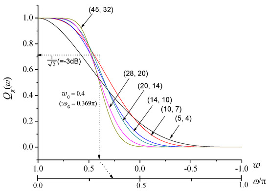
Figure 1. Maximally-flat (MAXFLAT) finite impulse response (FIR) filters: $Q_g\left(w\right)$ with various $N$ for $w_c=0.4$.

One of the main difficulties for MAXFLAT FIR filter design is to express the objective error function in a closed form [27]. This is due to the fact that the MAXFLAT FIR filter by any closed-form polynomial does not have any design (“free”) parameters. Thus, the objective error function has to be derived between the desired and actual variable frequency responses [23,29,30]. Referring to an objective function used in Reference [23], we can define a closed-form error compensation function $\mathsf{{\rm E}}\left(w\right)$ between a cut off-frequency fixing filter $Q\left(w\right)$ with a desired cut off point at $w=w_c$ and the closed-form polynomial filter $Q_g\left(w\right)$ of Equation (10).

$$\mathsf{{\rm E}}\left(w\right)=Q\left(w\right)-Q_g\left(w\right)=2^{2\left(N-K\right)}{C}_K{\left(\frac{1+w}{2}\right)}^K{\left(\frac{1-w}{2}\right)}^{N-K}$$

(16)

where $2^{2\left(N-K\right)}$ is for normalization and $C_K$ is a cut off-error compensation factor. Then, $C_K$ can be obtained in terms of $K$ and $w_c$ as:

$$C_K=\frac{\frac{1}{\sqrt{2}}-Q_g\left(w_c\right)}{2^{2\left(N-K\right)}{\left(\frac{1+w_c}{2}\right)}^K{\left(\frac{1-w_c}{2}\right)}^{N-K}}$$

(17)

by substituting $Q\left(w_c\right)=1/\sqrt{2}$ into the relation of Equation (16) with $w=w_c$. Consequently, adding $\mathsf{{\rm E}}\left(w\right)$ into $Q_g\left(w\right)$ can yield a “cutoff-error-free” filter $Q\left(w\right)$ with a cut off-frequency controllable by $C_K$:

$$Q\left(w\right)=Q_g\left(w\right)+\mathsf{{\rm E}}\left(w\right)={\left(\frac{1+w}{2}\right)}^K\left\{{\displaystyle \sum }_{i=0}^{N-K}\left(\begin{array}{c}K+i-1\\ i\end{array}\right){\left(\frac{1-w}{2}\right)}^i+2^{2\left(N-K\right)}{C}_K{\left(\frac{1-w}{2}\right)}^{N-K}\right\}$$

(18)

where Equation (18) consists of adding Equation (16) to Equation (10). More importantly, $Q\left(w\right)$ passes exactly through the desired cutoff point $w=w_c$, that is, $Q\left(w\right)$ always satisfies the cutoff condition, $Q\left(w_c\right)=1/\sqrt{2}$, regardless of the values of $K$ and $N$.

From Equation (18), it can be seen that $\mathsf{{\rm E}}\left(w\right)$ is added as an extra term to the $\left(N-K\right)$-th coefficient in the sum (of the second term of $Q_g\left(w\right)$ given in Equation (10)) without increasing the order of the filter. Then, small changes $\delta {g_i}^{\prime }s$ of the interpolation coefficients ${g_i}^{\prime }s$ in Equation (13) due to adding $\mathsf{{\rm E}}\left(w\right)$ can be obtained as:

$$\delta g_i={(-1)}^{N-K-i}{C}_K\left(\begin{array}{c}2\left(N-K\right)\\ i\end{array}\right),i=0,1,2,\dots ,N-K$$

(19)

by transforming Equation (16) into Equation (11). Hence, new ${{\widehat{g}}_i}^{\prime }s$ caused by adding $\mathsf{{\rm E}}\left(w\right)$ to $Q_g\left(w\right)$ consist of adding Equation (19) to Equation (13).

$${\widehat{g}}_i={(-1)}^{N-K-i}\left\{{\displaystyle \sum }_{\ell =0}^i\frac{1}{2^{2\left(N-K-\ell \right)}}\left(\begin{array}{c}N-l-1\\ K-1\end{array}\right)\left(\begin{array}{c}2\left(N-K\right)-2l\\ i-l\end{array}\right)+C_K\left(\begin{array}{c}2\left(N-K\right)\\ i\end{array}\right)\right\}$$

(20)

As shown in Equation (18), using $\mathsf{{\rm E}}\left(w\right)$ for the cut off-frequency error compensation of $Q_g\left(w\right)$ leads to a closed-form Chebyshev polynomial, which can characterize cut off-frequency fixing FIR filters as a “cut off-error free” in terms of $K$. However, the frequency response (i.e., $Q\left(cos\omega \right)$) of Equation (18) including Equation (16) no longer satisfies Equation (5). This is due to the fact that, for a given $N$ and $w_c$, there are $N$ different “cut off-error free” filters with $N$ different magnitudes responses caused by $N$ different $\mathsf{{\rm E}}\left(w\right)$ corresponding to $K=1$ to $N$. For this reason, if a wrong $\mathsf{{\rm E}}\left(w\right)$ (i.e., wrong $K)$ is chosen, it will have a negative effect on the flatness of $Q\left(w\right)$ even though $Q_g\left(w\right)$ is MAXFLAT. Hence, it is necessary to select $K$ exactly so that $\mathsf{{\rm E}}\left(w\right)$ compensates for the cutoff error of $Q_g\left(w\right)$ without damaging the flatness in the passband or the stopband.

3. The Order of Flatness (K)

In this section, $\mathsf{{\rm E}}\left(w\right)$ given in Equation (18) is analysed for building a computationally efficient and accurate solution to determine an optimal value of $K$ for a given $N$ and $w_c$.

As mentioned earlier, for the cut off-frequency error compensation of $Q_g\left(w\right)$ using $\mathsf{{\rm E}}\left(w\right)$ potentially leads to $Q\left(w\right)$ with its magnitude response exactly passing through the prescribed cutoff point $w=w_c$. However, the wrong choice of $K$ results in significant magnitude-distortions due to the undesired amplitude of the $\mathsf{{\rm E}}\left(w\right)$. Thus, to determine $K$ exactly, so that $\mathsf{{\rm E}}\left(w\right)$ compensates for the cut off-frequency error of $Q_g\left(w\right)$ without damaging the flatness, which is a simple and complete formula-based solution that has to be built on $\mathsf{{\rm E}}\left(w\right)$. Actually, in the case of Reference [23] using a distortion error function, they had proposed an iteration training method (see Figure 4 in Reference [23]) of estimating a minimum-distortion error function to determine $K$ for a given $N$ and $w_c$. However, this method has the disadvantage of requiring complicated and enormous computation processing for obtaining a suitable one among N different distortion error functions. This computation complexity increases rapidly with increasing N, which is the order of the filter. In addition, it sometimes has the frequency-response distortion by wrongly determining $K$. For this reason, a computationally efficient and accurate formula has to be needed for the design of such a filter.

From Equation (18), it is seen that $\mathsf{{\rm E}}\left(w\right)$ exhibits a “bell-curve-like” shape, which only has one peak gain, and zero gain at $w=\pm 1$ (corresponding to $\omega =0$ and $\omega =\pi$). Thus, the peak and inflection points of $\mathsf{{\rm E}}\left(w\right)$ can play important roles in identifying influential observations in terms of $K$ for a given $N$ and $w_c$. These points can be used to thoroughly characterize the effect of $\mathsf{{\rm E}}\left(w\right)$ on $Q\left(w\right)$ in terms of $K$. If $w_p$ is the peak point of $\mathsf{{\rm E}}\left(w\right)$, $w_p$ is given as:

$$w_P=\frac{2K-N}{N},-1<w_K<1$$

(21)

from $\partial \mathsf{{\rm E}}\left(w\right)/\partial w{|}_{w=w_P}=0$ and, then, the peak value $\mathsf{{\rm E}}\left(w_P\right)$ can be obtained in terms of $K$ as:

$$\mathsf{{\rm E}}\left(w_P\right)=C_K{\left(\frac{K}{N}\right)}^K{\left(1-\frac{K}{N}\right)}^{N-K}$$

(22)

by substituting Equation (21) into Equation (16) with $w_p$. In addition, letting $w_I^{+}$ and $w_I^{-}$ be two inflection points of $\mathsf{{\rm E}}\left(w\right)$, from ${\partial }^2\mathsf{{\rm E}}\left(w\right)/{\partial }^{2}w{|}_{w=w_I^{\pm }}=0,$ we can get:

$$w_I^{\pm }=\frac{-\left(2N-1\right)\left(N-2K\right)\pm \sqrt{N^2-4\left(1-4N\right)NK+4\left(1-4N\right)K^2}}{2N^2},-1<w_I^{\pm }<1$$

(23)

where $w_I^{\pm }$ (double signs in the same order) denotes $w_I^{+}$ and $w_I^{-}$, and $\mathsf{{\rm E}}\left(w_I^{\pm }\right)$ can also be obtained in terms of $K$ by substituting Equation (23) into Equation (16) with $w_I^{\pm }$. By substituting Equation (21) into Equation (23), $w_I^{\pm }$ can be rewritten in terms of $w_p$ as:

$$w_I^{\pm }=\left(1-\frac{1}{2N}\right)w_P\pm \frac{1}{2N}\sqrt{w_P^2-8K{w}_P+8K},-1<w_I^{\pm }<1$$

(24)

From Equation (24), it is seen that $w_I^{+}$ and $w_I^{-}$ are related to $w_p$ by:

$$\frac{w_I{}^{+}+w_I{}^{-}}{2}=\left(1-\frac{1}{2N}\right)w_P$$

(25)

and satisfy the inequality $w_I^{-}<w_P<w_I^{+}$. This means that the shape of $\mathsf{{\rm E}}\left(w\right)$ is not perfectly symmetric about the line $w=w_P$ and can lead to inequalities not only between $w_c$ and inflection points (i.e., $w_I^{-}$, $w_I^{+},$ and $w_p$) in terms of $K$ but also between $\mathsf{{\rm E}}\left(w_c\right)$ and inflection gains (i.e., $\mathsf{{\rm E}}\left(w_I^{-}\right)$, $\mathsf{{\rm E}}\left(w_I^{+}\right),$ and $\mathsf{{\rm E}}\left(w_p\right)$). For example, in the case of $w_c=0.4$ and $N=11$, Figure 2 shows $\mathsf{{\rm E}}{\left(w\right)}^{\prime }s$ corresponding to $K=3to10$ and the related parameters are indicated in Table 1, where $C_K$, $w_P$, and $w_I^{\pm }$ have been obtained according to Equations (17), (21) and (23). Figure 3 also shows $Q_g\left(w\right)$, $\mathsf{{\rm E}}\left(w\right)$, and $Q\left(w\right)$ for each case of the four ranges described in Table 1 where the prescribed cut off point $w_c$ falls into one of the following four ranges due to the choice of $K$: $w_c<w_I^{-}$, $w_I^{-}<w_c<w_P$, $w_P<w_c<w_I^{+},$ and $w_I^{+}<w_c$. From these examples, it can be found that the undesired magnitude of $\mathsf{{\rm E}}\left(w\right)$ around $w_p$ causes not only overshoot in the passband of $Q\left(w\right)$ if $w_c<w_P$(i.e., $w_c<w_I^{-}$ or $w_I^{-}<w_c<w_P$) for a given $K$, but also undershoot in the stopband if $w_I^{+}<w_c$. However, in these cases, $Q\left(w\right)$ can have a relatively narrow transition bandwidth due to $K$.

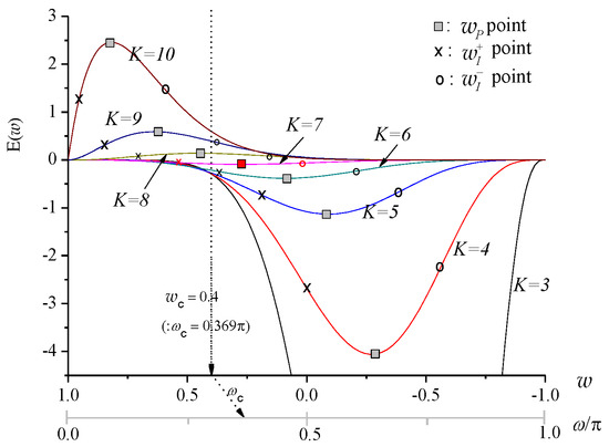
Figure 2. $\mathsf{{\rm E}}\left(w\right)$ due to increasing $K$ for $N=11$ and $w_c=0.4$ (${\omega }_c=0.369\pi$).

Table 1. Related parameters of Figure 2 and Figure 3.

Parameters	$\mathit{K}$
	3	4	5	6	7	8	9	10
CK	−0.1982	−0.3355	−0.5405	−0.7333	−0.4836	1.3807	6.7866	17.5271
$w_I^{-}$	−0.7032	−0.5507	−0.3871	−0.2135	−0.0300	0.1645	0.3731	0.6037
$w_P$	−0.4545	−0.2727	−0.0909	0.0909	0.2727	0.4545	0.6364	0.8182
$w_I^{+}$	−0.1645	0.0300	0.2135	0.3871	0.5507	0.7032	0.8418	0.9583
${\rm E}\left(w_c\right)$	−0.2923	−0.2886	−0.2713	−0.2147	−0.0826	0.1375	0.3944	0.5941
${\rm E}\left(w_I^{-}\right)$	−11.7403	−2.3584	−0.6661	−0.2284	−0.0550	0.0851	0.3615	1.5264
${\rm E}\left(w_P\right)$	−20.6230	−4.0613	−1.1314	−0.3837	−0.0915	0.1403	0.5898	2.4573
${\rm E}\left(w_I^{+}\right)$	−12.5099	−2.4404	−0.6733	−0.2259	−0.0531	0.0799	0.3236	1.1842
$w_c$	$w_I^{+}<w_c$				$w_P<w_c<w_I^{+}$	$w_I^{-}<w_c<w_P$		$w_c<w_I^{-}$
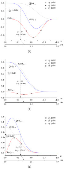
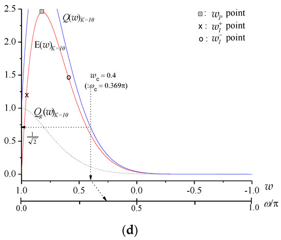
Example	-	-	Figure 3a	-	Figure 3b	-	Figure 3c	Figure 3d

Figure 3. $Q_g\left(w\right)$, $\mathsf{{\rm E}}\left(w\right)$, and $Q\left(w\right)$ and the relation between $\left(w_I^{\pm },w_P,w_c\right)$ due to $K$ for $N=11$ and $w_c=0.4$ (${\omega }_c=0.369\pi$): (a) $w_I^{+}<w_c$ as $K=5$, (b) $w_P<w_c<w_I^{+}$ as $K=7$, (c) $w_I^{-}<w_c<w_P$ as $K=9,$ and (d) $w_{\mathrm{c}}<w_I^{-}$ as $K=10$.

More importantly, it is shown that $Q\left(w\right)$ has a flat magnitude characteristic in both the passband and the stopband when $\mathsf{{\rm E}}\left(w_P\right)$ in terms of $K$ is negatively minimized, and, then, $w_c$ falls in between $w_P$ and $w_I^{+}$:

$$w_P<w_c<w_I^{+}$$

(26)

This corresponds to $K=7$ in Table 1 and, as shown in Figure 3b, no overshoot and no undershoot appear in the passband and the stopband. For the further evaluation of this result, in the case of $w_c=0.7071$ (corresponding to ${\omega }_c=0.25\pi$) and $N=28$, Figure 4a,b show $\mathsf{{\rm E}}\left(w\right)$ in terms of $K$ and the effect on $Q\left(w\right)$, respectively. The related parameters are also indicated in Table 2 where ${\delta }_O$ and ${\delta }_U$ are the peak values of overshoot and undershoot in the passband and the stopband, respectively. It can be seen that taking $K=23$ yields the smallest negative value $\mathsf{{\rm E}}\left(w_P\right){|}_{K=23}$ (at $w_P{|}_{K=23}=0.6429$) and results in $w_P{|}_{K=23}$ and $w_I^{+}{|}_{K=23}$ satisfying Equation (26) for a given $w_c=0.7071$. Consequently, using $K=23$ potentially leads to ${\rm E}\left(w\right){|}_{K=23}$ yielding a cut off-frequency fixing filter with zero overshoot and zero undershoot (i.e., ${\delta }_U={\delta }_O=0)$. Especially, it is shown that the filters by $K=22\mathrm{and}24$ have a tolerant magnitude distortion, but relatively narrower transition band than the filter by $K=23$.

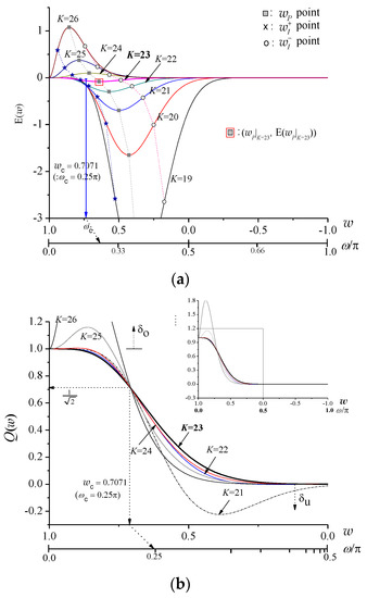
Figure 4. (a) $\mathsf{{\rm E}}\left(w\right)$ and (b) the effect of the related $\mathsf{{\rm E}}\left(w\right)$ on $Q\left(w\right)$ due to increasing $K$ for $N=28$ and $w_c=0.7071$ (${\omega }_c=0.25\pi$).

Table 2. Related parameters for Figure 4.

Parameters	$\mathit{K}$
	19	20	21	22	23	24	25	26
CK	−718.85	−475.26	−293.62	−151.91	−41.13	37.64	80.72	90.53
$w_I^{-}$	0.1741	0.2500	0.3272	0.4058	0.4862	0.5687	0.6539	0.7433
$w_P$	0.3571	0.4286	0.5000	0.5714	0.6429	0.7143	0.7857	0.8571
$w_I^{+}$	0.5274	0.5918	0.6550	0.7166	0.7766	0.8344	0.8894	0.9404
${\rm E}\left(w_c\right)$	−0.2882	−0.2776	−0.2499	−0.1884	−0.0743	0.0991	0.3097	0.5061
${\rm E}\left(w_I^{-}\right)$	−2.6494	−1.0075	−0.4267	−0.1832	−0.0510	0.0612	0.2316	0.6708
${\rm E}\left(w_P\right)$	−4.3577	−1.6531	−0.6983	−0.2990	−0.0829	0.0993	0.3738	1.0761
${\rm E}\left(w_I^{+}\right)$	−2.5816	−0.9755	−0.4101	−0.1746	−0.0480	0.0569	0.2106	0.5861
${\delta }_o$	0.0	0.0	0.0	0.0	0.0	0.0058	0.1594	0.8101
${\delta }_u$	−3.7859	−1.1088	−0.2241	−0.0021	0.0	0.0	0.0	0.0
$w_c$	$w_I^{+}<w_c$			$w_P<w_c<w_I^{+}$		$w_I^{-}<w_c<w_P$		$w_c<w_I^{-}$

From the results so far, it has been shown that $K$ has to be chosen so that $w_P$ and $w_I^{+}$ of $\mathsf{{\rm E}}\left(w\right)$ satisfy the condition of Equation (26) for the prescribed cut off point $w_c$. To determine an optimal value of $K$ under this condition, substituting $w_P$ and $w_I^{+}$ given by Equations (21) and (23) into Equation (26) and simplifying the algebra, yields:

$$\frac{2N+\left(2N-1\right)w_c-\sqrt{4N+\left(1-4N\right)w_c^2}}{4}<K<\frac{N\left(1+w_c\right)}{2},forintegerK$$

(27)

Hence, we can infer from Equation (27) that the empirical formula of Equation (15) given by Hermann is a wrong expression since $K$ in accordance with Equation (15) does not satisfy the condition Equation (26) (i.e., $w_P<w_c$). From the fact that choosing the optimal value of $K$ has to satisfy Equation (27), a new formula that is more accurate than Equation (15) can be defined as:

$$K=\left[\frac{4N-\left(1-4N\right)w_c-\sqrt{4N+\left(1-4N\right)w_c^2}}{4}+0.5\right]$$

(28)

by averaging the upper and lower limit values of Equation (27). To verify the effectiveness of this formula, Figure 5 shows the accuracy comparison of Equations (15) and (28) for $w_c=0.4$ (${\omega }_c=0.369\pi$) and $w_c=0.7071$ (${\omega }_c=0.25\pi$) where the “★” symbol denotes the optimal $K$ chosen by negatively minimizing $\mathsf{{\rm E}}\left(w_P\right)$ under condition (27). This indicates that $Ks$ obtained according to Equation (28) are remarkably consistent with the optimal $Ks$.

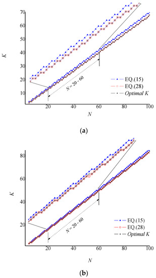
Figure 5. Accuracy comparison of Equations (15) and (28) due to $N$ for (a) $w_c=0.4$ (${\omega }_c=0.369\pi$) and (b) $w_c=0.7071$ (${\omega }_c=0.25\pi$).

Based on results so far, Figure 6 exhibits a design procedure to directly compute the coefficients of cut off-frequency fixing filters with a desired frequency response. Table 3 and Figure 7 show the comparison between the proposed method and existing methods [15,23] for $N=20$ and $45$. From Table 3, it can be said that the proposed filters apparently are a “cut off error free” and “flat magnitude” since ${\delta }_o<{10}^{-14}$ can be very negligible and ignored. On the other hand, previous filters using empirical formula of Equation (15) are maximally flat in the passband and stopband, while there exists a filter cut off-frequency error of 2.2% to 6.6%. In addition, it appears that the iteration training method [23] leads to very slight cut off errors despite performing multiple computations to determine K, as shown in Figure 4 in Reference [23]. Consequently, these examples demonstrate that the proposed method derives accurate FIR filters with a magnitude response while allowing direct and simple computation in designing such a filter.

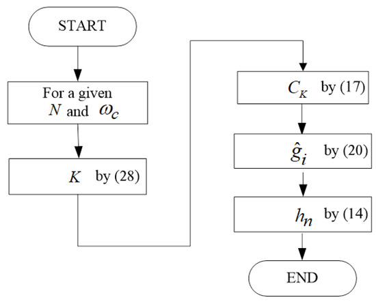
Figure 6. Design procedure of cut off-frequency fixing filters.

Table 3. Comparison of three design methods for (a) $N=20$ and (b) $N=45$.

Parameters		${\mathit{\omega }}_{\mathit{c}}=\mathbf{0.369}\mathit{\pi }\left({\mathit{w}}_{\mathit{c}}=\mathbf{0.4}\right)$			${\mathit{\omega }}_{\mathit{c}}=\mathbf{0.25}\mathit{\pi }\left({\mathit{w}}_{\mathit{c}}=\mathbf{0.7071}\right)$
		MAXFLAT Filters of Equation (10)	Reference [23]	Cutoff Fixing Filters of Equation (18)	MAXFLAT Filters of Equation (10)	Reference [23]	Cutoff Fixing Filters of Equation (18)
$N=20$	${\omega }_{3dB}{}^1$	0.3502π	0.3690π	0.3690π	0.2419π	0.25π	0.25π
	$\left({\omega }_c-{\omega }_{3dB}\right)/\mathsf{\pi }$2	0.0188	2.14 × 10−5	0.0	0.0081	0.0	0.0
	${\delta }_o{}^3$	0.0	0.0	0.0	0.0	0.0	0.0
	${\delta }_u$	0.0	0.0	0.0	0.0	0.0	0.0
	K decision	Equation (15)	training (13 iteration)	Equation (28)	Equation (15)	training (16 iterations)	Equation (28)
	accuracy/complexity 4	low/low	high/very high	high/low	low/low	high/very high	high/low
$N=45$	${\omega }_{3dB}{}^1$	0.3445π	0.3690π	0.3690π	0.2445π	0.25π	0.25π
	$\left({\omega }_c-{\omega }_{3dB}\right)/$ π	0.0245	3.14 × 10−7	0.0	0.0055	1.83 × 10−12	0.0
	${\delta }_o{}^3$	0.0	0.0	3.11× 10−15	0.0	0.0	4.44 × 10−16
	${\delta }_u$	0.0	0.0	0.0	0.0	0.0	0.0
	K decision	Equation (15)	training (30 iteration)	Equation (28)	Equation (15)	training (37 iterations)	Equation (28)
	accuracy/complexity 4	low/low	high/very high	high/low	low/low	high/very high	high/low

¹${\omega }_{3dB}$ denotes the actual cut off-frequency of the filter. ² $\left({\omega }_c-{\omega }_{3dB}\right)/\mathsf{\pi }$ indicates the cut off-frequency error of the filter. ³ ${\delta }_o$ was calculated to sixteen decimal places. ⁴ this denotes K decision accuracy and computation complexity.

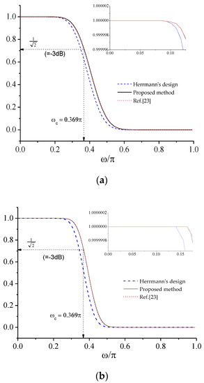
Figure 7. Comparison of three design methods: (${\omega }_c=0.369\pi$) for (a) $N=20$ and (b) $N=45$.

Figure 8, using Figure 6, shows cut off-frequency fixing filters for ${\omega }_c=0.369\pi$ ($w_c=0.4$) and various $N$, and the related values are given in Table 4. Table 5 also indicates coefficients of the cut off-frequency fixing filter for $\left(N,K\right)=\left(20,13\right)$, where ${\widehat{g}}_i$ and $h_n$ have been obtained according to Equations (20) and (14), respectively.

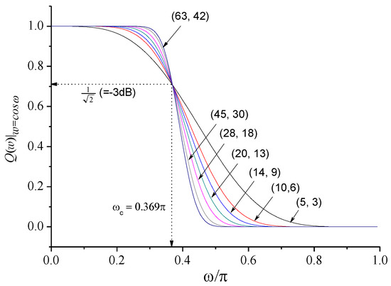
Figure 8. Cut off-frequency fixing filters with various $N$ and ${\omega }_c=0.369\pi$ ($w_c=0.4$).

Table 4. Related parameters of Figure 8.

Parameters	N
	10	14	20	28	45	63
$K$	6	9	13	18	30	42
$C_K$	−0.5846	−0.7311	−1.8770	−10.073	−112.62	−4055.5
$w_P$	0.2000	0.2857	0.3000	0.2857	0.3333	0.3333
$w_I^{+}$	0.5000	0.5318	0.5059	0.4618	0.4702	0.4495

Table 5. Coefficients of the cut off-frequency fixing filter for $\left(N,K\right)=\left(20,13\right)$.

${{\mathit{g}}_{\mathit{i}}}_{}$	${\mathit{h}}_{\mathit{n}}$
$g_0$= −1.198409231	h0 = −0.000000018	h11 = −0.003859813
$g_1$= 21.309955797	h1 = −0.000000147	h12 = −0.005450869
$g_2$= −169.484927527	h2 = −0.000000073	h13 = 0.005958058
$g_3$= 802.886975733	h3 = 0.000003072	h14 = 0.020963265
$g_4$= −2532.615452798	h4 = 0.000011169	h15 = 0.004171941
$g_5$= 5615.229929033	h5 = −0.000003022	h16 = −0.048651840
$g_6$= −8988.135420893	h6 = −0.000097254	h17 = −0.055049249
$g_7$= 10,505.014699770	h7 = −0.000159706	h18 = 0.078213381
	h8 = 0.000280582	h19 = 0.297774354
	h9 = 0.001164512	h20 = 0.408751644
	h10 = 0.000355835

All coefficients were rounded off to nine decimal places.

4. Conclusions

Problems with the cut off-frequency error always arise in a MAXFLAT filter design. This is due to the fact that the maximum possible number of zeros at $z=\pm 1$ is imposed, which leaves no degree of freedom, and, thus, no independent parameters. In this paper, a new method has been proposed providing a cut off-frequency error compensation function, available to previous closed-form polynomials, for compensating for the cut off-frequency error of MAXFLAT FIR filters. It has been shown that this error compensation function derives a closed-form Chebyshev polynomial characterizing cut off fixing FIR filters with a prescribed cut off-frequency and allows a computationally efficient and accurate formula to obtain such filters with flat magnitude response characteristics for a given order of a filter and cut off-frequency. The examples were shown to provide a complete and accurate solution for the design of such filters. Hence, a solution to the problem encountered in the previous methods is found.

References

- Zhao, H.; Zhang, L.; Liu, J.; Zhang, C.; Cai, J.; Shen, L. Design of a Low-Order FIR Filter for a High-Frequency Square-Wave Voltage Injection Method of the PMLSM Used in Maglev Train. Electronics 2020, 9, 729. [Google Scholar] [CrossRef]
- Kalpun, D.; Butusov, D.; Ostrovskii, V.; Veligosha, A.; Gulvanskii, V. Optimization of the FIR filter structure in finite residue field algebra. Electronics 2018, 7, 372. [Google Scholar]
- Vaidyanathan, P. Efficient and multiplierless design of FIR filters with very sharp cutoff via maximally flat building blocks. IEEE Trans. Circuits Syst. 1985, 32, 236–244. [Google Scholar] [CrossRef]
- Vaidyanathan, P. Optimal design of linear phase FIR digital filters with very flat passbands and equiripple stopbands. IEEE Trans. Circuits Syst. 1985, 32, 904–917. [Google Scholar] [CrossRef]
- Samadi, S.; Nishihara, A. The world of flatness. IEEE Circuits Syst. Mag. 2007, 7, 38–44. [Google Scholar] [CrossRef]
- Ping, Z.; Chun, Z. Four-Channel Tight Wavelet Frames Design Using Bernstein Polynomial. Circuits Syst. Signal Process. 2012, 31, 1847–1861. [Google Scholar]
- Huang, X.; Jing, S.; Wang, Z.; Xu, Y.; Zheng, Y. Closed-form FIR filter design based on convolution window spectrum interpolation. IEEE Trans. Signal Process. 2015, 64, 1173–1186. [Google Scholar] [CrossRef]
- Huang, X.; Wang, Y.; Yan, Z.; Xian, H.; Liu, M. Closed-form FIR filter design with accurately controllable cut-off frequency. Circuits Syst. Signal Process. 2017, 36, 721–741. [Google Scholar] [CrossRef]
- Tseng, C.C.; Lee, S.L. Closed-form designs of digital fractional order Butterworth filters using discrete transforms. Signal Process. 2017, 137, 80–97. [Google Scholar] [CrossRef]
- Roy, S.; Chandra, A. On the Order Minimization of interpolated Bandpass Method Based Narrow Transition Band FIR Filter Design. IEEE Trans. Circuits Syst. I Reg. Pap. 2019, 66, 4287–4295. [Google Scholar] [CrossRef]
- Huang, X.; Zhang, B.; Qin, H.; An, W. Closed-form design of variable fractional-delay FIR filters with low or middle cutoff frequencies. IEEE Trans. Circuits Syst. I Reg. Pap. 2017, 65, 628–637. [Google Scholar] [CrossRef]
- Kušljević, M.D.; Tomić, J.J.; Poljak, P.D. Maximally Flat-Frequency-Response Multiple-Resonator-Based Harmonic Analysis. IEEE Trans. Instrum. Meas. 2017, 66, 3387–3398. [Google Scholar] [CrossRef]
- Yoshida, T.; Aikawa, N. Low-Delay Band-Pass Maximally Flat FIR Digital Differentiators. Circuits Syst. Signal Process. 2018, 37, 3576–3588. [Google Scholar] [CrossRef]
- Roy, S.; Chandra, A. Design of narrow transition band variable bandwidth digital filter. IET Circuits Devices Syst. 2020, 14, 750–757. [Google Scholar] [CrossRef]
- Herrmann, O. On the approximation problem in nonrecursive digital filter design. IEEE Trans. Circ. Theory 1971, 18, 411–413. [Google Scholar] [CrossRef]
- Miller, J.A. Maximally flat nonrecursive digital filters. Electron. Lett. 1972, 8, 157–158. [Google Scholar] [CrossRef]
- Rajagpoal, L.; Roy, S.C.D. Design of maximally-flat FIR filters using the Bernstein polynomial. IEEE Trans. Circuits Syst. 1987, 34, 1587–1590. [Google Scholar]
- Fahmy, M.F. Maximally flat non-recursive digital filters. Int. J. Circuit Theory Appl. 1976, 4, 311–313. [Google Scholar] [CrossRef]
- Bromba, M.U.A.; Ziegler, H. Explicit formula for filter function of maximally flat nonrecursive digital filters. Electron Lett. 1980, 16, 905–906. [Google Scholar] [CrossRef]
- Thajchayapong, P.; Puangpool, M.; Banjongjit, S. Maximally Flat FIR filters with prescribed cut-off frequency. Electron. Lett. 1980, 16, 514–515. [Google Scholar] [CrossRef]
- Roy, S.C.D. A New Chebyshev-like Low-pass Filter Approximation. Circuits Syst. Signal Process. 2010, 29, 629–636. [Google Scholar]
- Rajagpoal, L.; Roy, S.C.D. Optimal design of maximally flat FIR filters with arbitrary magnitude specifications. IEEE Trans. Acoust. Speech Signal Process. 1989, 37, 512–518. [Google Scholar] [CrossRef]
- Jeon, J.; Kim, D. Design of nonrecursive FIR filters with simultaneously MAXFLAT magnitude and prescribed cutoff frequency. Digital Signal Process. 2012, 22, 1085–1094. [Google Scholar] [CrossRef]
- Lian, Y.; Yu, Y.J. Guest Editorial: Low-Power Digital Filter Design Techniques and Their Applications. Circuits Syst Signal Process. 2010, 29, 1–5. [Google Scholar] [CrossRef][Green Version]
- Vlcek, M.; Unbehauen, R. Analytical solution of design for IIR equiripple filters. IEEE Trans. Acoust. Speech Signal Process. 1989, 37, 1518–1531. [Google Scholar] [CrossRef]
- Kaiser, J.F. Comments on maximally flat nonrecursive digital filters. Int. J. Circuit Theory Appl. 1977, 5, 103. [Google Scholar] [CrossRef]
- Jinaga, B.C.; Roy, S.C.D. Explicit formulas for the Weighting coefficients of maximally flat nonrecursive digital filters. Proc. IEEE. 1984, 72, 1092. [Google Scholar] [CrossRef]
- Jinaga, B.C.; Roy, S.C.D. Explicit formula for the coefficients of maximally flat nonrecursive digital filter transfer function expressed in powers of cos w. Proc. IEEE. 1985, 73, 1135–1136. [Google Scholar] [CrossRef]
- Kumar, B.; Kumar, A. Efficient linear-phase FIR, maximally flat error approximations for the amplitude response |1/ωr|, r = 1, 2, 3, …, and a versatile realization. Circuits Syst. Signal Process. 2000, 19, 567–580. [Google Scholar] [CrossRef]
- Vesma, J.; Saramaki, T. Polynomial-Based Interpolation Filters—Part I: Filter Synthesis. Circuits Syst. Signal Process. 2007, 26, 115–146. [Google Scholar] [CrossRef]
Publisher’s Note: MDPI stays neutral with regard to jurisdictional claims in published maps and institutional affiliations. |
© 2021 by the authors. Licensee MDPI, Basel, Switzerland. This article is an open access article distributed under the terms and conditions of the Creative Commons Attribution (CC BY) license (http://creativecommons.org/licenses/by/4.0/).