Abstract
The next-generation networks (5G and beyond) require robust channel codes to support their high specifications, such as low latency, low complexity, significant coding gain, and flexibility. In this paper, we propose using a fountain code as a promising solution to 5G and 6G networks, and then we propose using a modified version of the fountain codes (Luby transform codes) over a network topology (Y-network) that is relevant in the context of the 5G networks. In such a network, the user can be connected to two different cells at the same time. In addition, the paper presents the necessary techniques for analyzing the system and shows that the proposed scheme enhances the system performance in terms of decoding success probability, error probability, and code rate (or overhead). Furthermore, the analyses in this paper allow us to quantify the trade-off between overhead, on the one hand, and the decoding success probability and error probability, on the other hand. Finally, based on the analytical approach and numerical results, our simulation results demonstrate that the proposed scheme achieves better performance than the regular LT codes and the other schemes in the literature.
1. Introduction
With the advent of the fifth generation (5G) of the 3GPP mobile communication standard, it is expected that major content distributors (e.g., Google, Facebook, etc.) will exploit the network capabilities to provide and retrieve massive amounts of data. For instance, the Youtube platform, one of Google’s subsidiaries, receives more than 500 h of uploaded fresh video per minute, 173,611 h being watched per minute, and 722 million h were live-streamed in the first quarter of 2019 [1]. These companies store these huge amounts of data in many different places to avert a data storage disaster, enhance the latency, and avoid an outage. Once a particular user attempts to download content that is available from two sources, in this sense, half of the information can come from one source and the other half from another source. For example, a simple application might be video conferencing with three users. In such a scenario, one user needs to receive video feeds from two independent sources. For each example given, there may exist a common intermediate/transport node. As a result, one of the main features of the 5G network is the dual connectivity (DC), where the user has connections with two different base stations or two different generations (e.g., 4G and 5G) simultaneously [2,3]. By empowering the DC, the overall system performance will be enhanced [4,5]. For example, the data rate of the mobile user is increased, the number of handover interruptions is decreased, and the probability of disconnectivity, which appears because of the small cell size in the 5G network, is significantly decreased [4,6]. In all the aforementioned applications, a reasonable model to adopt is the so-called Y-network [7].
The Y-network consists of two source nodes and , the destination node D, and the intermediate sender–receiver pair that acts as relay R to facilitate the communication between the sources and the destination, as shown in Figure 1. However, it is essential to realize that there is no direct link between the two sources. In addition, the three communication links are assumed to have orthogonal resources such as frequency or timeslot. As a result, there will be no collisions on such a network. Moreover, these three links are modeled as binary erasure channels (BECs) with different erasure probabilities.
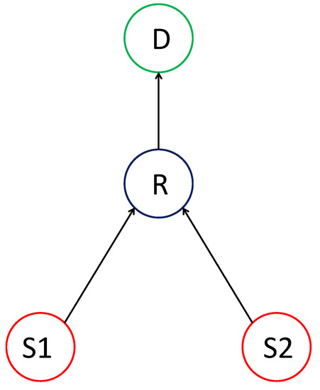
Figure 1.
The Y-network topology.
In the fountain codes, the transmitter sends a stream of encoded symbols over the channel and then adjusts the number of encoded symbols (i.e., code rate) depending on the channel’s properties. Such a process is achieved without prior knowledge of the channel’s properties (e.g., CSI) at the transmitter. In other words, fountain codes can work in the absence of a feedback channel, even in nasty channels [8,9,10]. Such codes work on erasure channels such as binary erasure channels (BECs) [9,11,12], as well as noisy channels such as AWGN channels [13,14,15] and fading channels [16,17].
In practice, Luby transform (LT) codes [9] and Raptor codes [18], which are the most well-known and widely used fountain codes, are utilized to enrich the transmission efficiency of the point-to-point communications. LT codes can potentially generate an endless number of encoded bits/symbols from the source data and then send these encoded bits/symbols to the destination. Once the destination receives an adequate number of encoded bits, it can decode them and obtain the source bits. Therefore, one of the most essential design parameters of LT codes is the degree distribution that defines the encoding and decoding complexities. Luby proposes two types of distributions, namely ideal soliton distribution (ISD) and robust soliton distribution (RSD) [9]. Additionally, shaping the left degree distribution (i.e., the degrees of the source nodes) of LT codes improves the performance of the point-to-point communications [19]. Hence, this algorithm is referred to as memory-based-LT (MBLT).
Recently, the concept of distributed fountain codes (DFC) has been used to send data from multiple sources to a destination through a common relay [20,21,22,23,24]. However, the concept of DFC deals with sources of different data. Therefore, to deal with sources of the same data in the Y-network topology (Figure 1), we propose using the MBLT codes in both sources and then using a buffer-and-forward (BF) strategy at the relay. Moreover, the proposed scheme can be used in other topologies, such as a multi-source single-sink relay network with an arbitrary number of sources [25,26,27].
In this paper, we analyze coding schemes for the Y-network. Then, we present a novel approach to designing LT code over the Y-network where the concept of memory-based is applied at both sources, and then the relay uses a buffer-and-forward strategy. The proposed scheme reduces the latency and complexity and improves the error probability to meet the fundamental requirements of 5G and the applications shown above. Furthermore, our proposed approach is not restricted to the regular LT codes but can adapt to any desired degree distribution. To test the validity of the proposed approach, we derive the decoding success probability (DSP) for the Y-networks. Furthermore, we use a novel technique of optimizing the codes’ parameters that maximize the derived DSP. Finally, we compare our proposed scheme’s DSP and error probability with different works presented in the literature using the same settings.
This paper is organized as follows. In Section 2, we provide a brief review of the encoding and decoding processes of LT codes and review the related works. Next, the proposed algorithm of using the concept of the MBLT in the Y-network is presented in Section 3. Then, the performance analyses of regular LT codes and the proposed scheme are provided in Section 4. Subsequently, the numerical results of optimizing the LT codes and the proposed schemes are shown in Section 5. Finally, we conclude the paper in Section 6.
2. Preliminaries and Related Work
LT codes are the first practical realization of fountain codes invented by Michael Luby [8,9]. Asymptotically, they are optimal in every erasure channel (e.g., BEC) in terms of capacity achievement. Note that the BEC channel is a simple communication channel, where the receiver receives the transmitted bit/symbol correctly or does not receive it (i.e., erased) with a probability . This probability is referred to as erasure probability.
2.1. LT Encoding Process
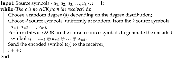
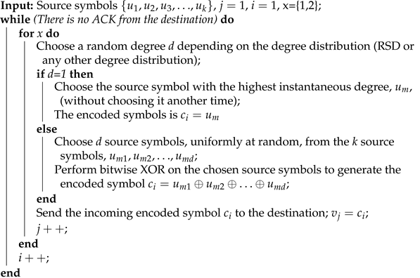
Assume that k input symbols, , are to be transmitted: the transmitter determines and sends a potentially limitless stream of encoded symbols, as shown in Algorithm 1 [9]. In the algorithm, are d input symbols chosen uniformly from the k input symbols, and is the encoded symbol at step i. As can be seen from the algorithm, the encoding process keeps generating encoded symbols until a positive acknowledgment (ACK) is collected from the receiver. This is how the LT codes adjust their codes depending on the channel’s characteristics. For instance, channels with a high loss rate require more encoded symbols, producing a low code rate. At the same time, channels with a low loss rate require fewer encoded symbols, resulting in a high code rate.
| Algorithm 1: Encoding Process of LT Codes |
 |
After applying Algorithm 1 on the k source symbols, encoded symbols are generated on the fly, as shown in Figure 2, where is the code overhead.
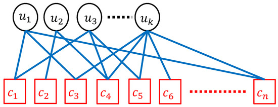
Figure 2.
The encoding process of LT codes, where k source symbols (circles) are used to generate n encoded symbols (squares).
2.2. LT Decoding Process
In the decoding process at the receiver, the decoder uses the Gaussian elimination (GE) process to decode the received symbols and regenerate the source symbols. However, the GE decoder requires high computational complexity; specifically, for n received encoded symbols, the decoder requires . As a result, Luby proposed a new decoding process called belief propagation (BP), used in LT codes [28]. The BP decoder enables a low-complexity decoding process. Thus, it turns out that the complexity of BP is only . The decoding process of the BP is shown in Algorithm 2 [28].
| Algorithm 2: BP Decoding Process of LT Codes |
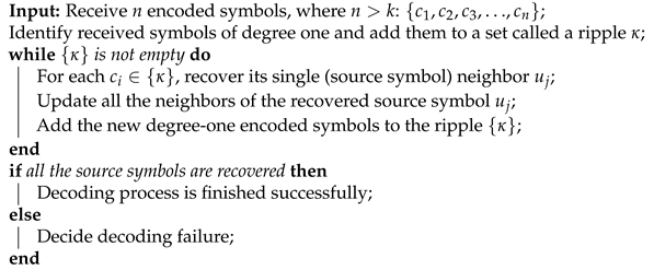 |
Figure 3 illustrates a toy example of the BP decoding process. In the example, there are four source symbols and six encoded symbols. In the beginning, the decoder finds the degree-one encoded symbols , and then its source symbol neighbor is recovered immediately (i.e., ), as shown in Figure 3a. Then, all the encoded symbol neighbors of the recovered source symbol will be updated: and . Then, their connected edges to the recovered source symbols will be removed, as shown in Figure 3b. Repeatedly, the decoder searches for a degree-one encoded symbol, which is in this case. Now, the encoded symbol is recovered, . Then, the encoded symbol is updated , and its connected edge to is removed. Consequently, is recovered , as depicted in Figure 3c. Likewise, encoded symbols and , which are neighbors of , are updated; and , and their connected edges to , are removed. Finally, the source symbol is recovered; , as shown in Figure 3d.
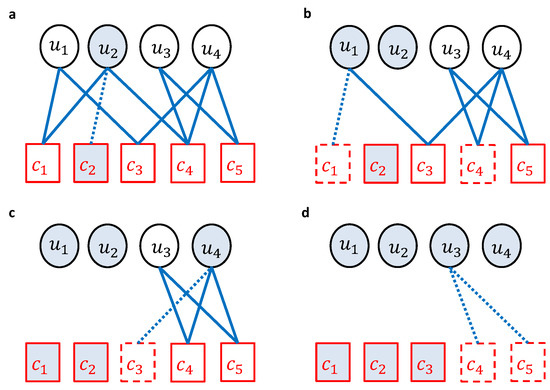
Figure 3.
A toy example of an LT decoding process, where there are 4 source symbols (circles) and 5 encoded symbols (squares). Figures from (a–d) show the decoding steps of the example.
2.3. Degree Distributions of LT Codes
As can be seen from the encoding and decoding processes of LT codes, the degree distribution significantly influences LT codes’ performance [9,29]. As a result, designing an optimal degree distribution is crucial for code performance, such as the code rate, reliability, complexity, and decoding success probability (DSP). The first ‘degree distribution’ was designed by Luby, and it is referred to as ideal soliton distribution (ISD), , and it is given as [9]:
Note that the ISD is the optimal distribution in terms of the code rate, where only k encoded symbols are required to recover the k source symbols. Thus, only one source symbol is recovered at each decoding step. Simultaneously, a new encoded symbol will be changed to have only one neighbor. That is, there is only one degree-one encoded symbol at a time. In practice and while using the BEC, if any encoded symbol is erased, this will stop the decoder’s peeling process, and then the decoder will announce decoding failure. To overcome this problem of the ISD, Luby introduced another degree distribution called robust soliton distribution (RSD), , where the expected number of degree-one encoded symbols is increased from 1 to R (). Thus, RSD requires more encoded symbols (i.e., ) but is asymptotically optimal in terms of capacity-achieving and practical. Moreover, its average degree distribution is . The RSD, , is given by [9]:
where is used for normalization and is given by
where is the modified ripple size, is a suitable constant, and is the allowable failure probability of the decoder once it receives n encoding symbols. As one can notice, there is a spike at the position of .
As a result, the LT code can be defined as its parameters , where .
The probability of decoding failure, , is calculated as the probability that a given source symbol is not covered at the encoding process, and it is given by [18]
where is the first derivative of the degree distribution . Thus, is the average degree of the encoded symbols.
3. Y-Network Using MBLT Algorithm
In this section, we propose using the MBLT algorithm as a coding technique in the Y-network (Figure 1) in order to enhance the performance. The encoding and decoding processes of the MBLT algorithm are shown in the following subsections.
3.1. Encoding Process of the MBLT on the Y-Network
Initially, shaping the left degree distribution (i.e., MBLT) is presented to point-to-point communications where a single transmitter sends data to a single receiver [19]. In our proposed scheme, we use the concept of the memory-based over the Y-network, where two encoding processes have to be done: one encoding process at each source. Then, the relay applies the buffer-and-forward (BF) strategy to the incoming encoded symbols. The encoding process of the proposed approach over the Y-network is given in Algorithm 3. In the algorithm, x shows the number of sources, is the encoded symbol at each source, and is the encoded symbol from the relay to the destination.
Naturally, the encoding process is similar to the conventional encoding process of LT codes using the RSD distribution. The only difference is shown once the picking degree is ; the single source symbol is chosen uniformly from the k source symbols in the regular LT encoding. In contrast, the single source symbol, which has the highest instantaneous degrees, is chosen without repetition when using the proposed algorithm. The reason behind this is the importance of the degree-one encoded symbols (i.e., the ripple). They are essential in initiating the decoding process and keeping it going until the entirety of the source symbols are recovered. Indeed, as the source symbols connected to the ripple have high degrees, the encoding process recovers the source symbols faster and with high efficiency.
| Algorithm 3: MBLT encoding process at the Y-network. |
 |
3.2. Decoding Process of MBLT Algorithm
As shown in the previous section, the encoding process of the MBLT codes is similar to regular LT codes. As a result, the shaping of the right degree distribution is intact. Hence, the BP algorithm can still be used, as shown in Algorithm 2. However, the MBLT focuses on the degree-one encoded symbols, which are essential to kick-start the decoding process and keep the complexity at the lowest. Under these circumstances, the BP algorithm in the MBLT case will be much faster and more effective than the regular LT codes.
4. Performance Analysis
This section provides efficient methods of analyzing the proposed scheme. In the first instance, we develop the use of decoding success probability (DSP) to investigate the performance of the regular LT codes as well as the proposed scheme. Then, we use the DSP to optimize the parameters of the regular LT codes.
4.1. Decoding Success Probability
In this subsection, we study the performance of LT codes in terms of decoding success probability (DSP). In general, we use the analysis proposed by Karp et al. to measure the DSP [29,30]. In brief, the analysis defines three main parameters at each decoding step: (1) the number of unrecovered source symbols at this step, u; (2) the ripple, r, which is the number of degree-one encoded symbols at this step; (3) the cloud, c, which is the number of output symbols that have a degree higher than one at this step. Thus, the decoder will be in state () with probability , which is given by Equation (5) (at the bottom of the page). in the equation is the transition probability from state to state , and it is given by Equation (6) (at the bottom of the page). Finally, in Equation (6) represents the probability of releasing a degree-one encoded symbol from the cloud (c) given that there are u unrecovered source symbols, and it is given by Equation (7) (at the bottom of the page).
The decoder fails to recover all the source symbols once it approaches a state of and . Thus, for a given degree distribution, (such as RSD) and n received encoded symbols, the DSP is given by
4.2. Optimization of LT Code Parameters
In this subsection, we propose a novel optimization model that aims to find parameters c and (which define the RSD distribution of the LT codes) to maximize the DSP. Depending on the DSP obtained in the previous subsection, we propose a new optimization model to design the parameters of LT codes. The proposed optimization model is formulated in Equation (9).
where the number of received symbols n is fixed. The last two constraints are obtained by sitting the spike position (i.e., ) between the two extreme cases. That is, .
5. Numerical Results
In this section, we investigate the performance of the regular LT codes and the proposed scheme. First, we show the results of optimizing the regular LT codes. Then, we compare the results of regular LT codes and the proposed scheme in terms of two performance measures—specifically, DSP and BER. In addition, the three channels in the Y-network are modeled as BECs. Namely, the first erasure channel is between the first source and the relay with an erasure probability of , the second erasure channel is between the second source and the relay with an erasure probability of , and the third erasure channel is between the relay and the destination with an erasure probability of . Note that all of the performance measurements of the proposed scheme and the conventional schemes are implemented and evaluated using the MATLAB R2015a platform.
5.1. LT Parameters
This subsection optimizes LT codes’ parameters (i.e., c and ) depending on the optimizing model, Equation (9), shown in Section 4.2. The simulation results are run over 10,000 transmissions in each scheme to obtain averages of the implementation measurements. Furthermore, all three channels in the Y-network are assumed to have an erasure probability of .
Figure 4 shows the DSP of LT codes versus the overhead () at for different values of and (Figure 4a), (Figure 4b), (Figure 4c), and (Figure 4d). As a matter of fact, the best c and values depend on the code length k and the overhead, (or, equivalently, the number of received symbols n). However, as the value of c increases, the performance of DSP will be decreased. Thus, it approaches 100% slower. Therefore, at packet length and overhead , the best value of c is around , and the best value of is around .
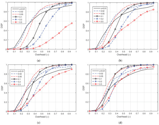
Figure 4.
Decoding success probability (DSP) versus the overhead () for LT codes of at different values of c and . (a) . (b) . (c) . (d) .
Likewise, Figure 5 shows the DSP of LT codes versus the overhead () but at . In general, the performance at is better than the performance at . Moreover, the same observations as in the case of are obtained. As the value of c increases, the DSP performance becomes worse. Similarly, the best value of c is around , and the best value of is around .
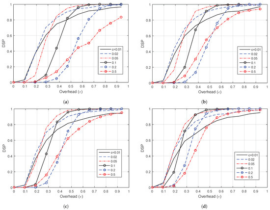
Figure 5.
DSP versus the overhead () for LT codes of at different values of c. (a) . (b) . (c) . (d) .
Fundamentally, the parameter shows the failure probability of the decoder after it receives n encoded symbols [9]. In addition, the value shows how much the generator matrix is sparse. Thus, as increases, the average degree of the encoded symbols is decreased. Therefore, there is a trade-off between the failure probability and the average degree of the encoded symbols (i.e., complexity). Further, the c parameter is a positive constant that highly affects the performance of the code. Thus, if c increases, the probability of degree-one encoded symbols is increased (which is very important to start the decoding process). However, simultaneously, the average degree of the encoded symbols and the complexity increase. In summary, we choose and as the optimal values in terms of the DSP in the rest of our work.
5.2. DSP and BER
In this subsection, we investigate the performance of our proposed MBLT codes in the Y-network. We use the proposed scheme over the regular LT codes. We also use the memory-based concept over one of the well-known distributions in the literature called decreasing ripple size distribution (DRSD) [31]. Thus, our scheme over the DRSD is referred to as memory-based DRSD (MBDRSD).
The length of source symbols is set to k at each source. Both DSP and BER measurements at different k and overhead over the BEC channel with different erasure probabilities are presented. All the simulation results are run over 100,000 transmissions in each scheme to obtain averages of the implementation measurements.
Figure 6 shows the DSP versus the overhead, , for four different schemes. The figure is obtained at a packet length of , and the optimized parameters of the RSD and . In order to check the improvement of the proposed algorithm without the effect of the channel characteristics, the erasure probabilities of the three channels in the Y-network are set to zero (i.e., all three channels are clear). As the figure shows, the DSP increases and approaches 100% as the overhead increases (i.e., the number of received symbols increases). However, the faster the scheme approaches 100%, the better the scheme. Moreover, we can observe from the figure that applying the proposed scheme over the traditional LT code with the optimized RSD parameters enhances the performance. In addition, the DRSD scheme outperforms the traditional LT codes with RSD distribution. Nevertheless, applying the concept of memory based on DRSD (i.e., MBDRSD) enhances the performance in terms of the DSP. Although the DSPs of MBDRSD and DRSD almost coincide, MBDRSD surpasses DRSD in terms of BER, as shown in the following figures.
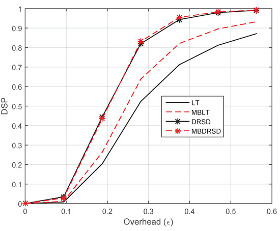
Figure 6.
DSP versus the overhead () for different coding schemes at and erasure probabilities of , , and .
In a similar manner, Figure 7 shows the error probability (i.e., BER) versus the code overhead () for the four schemes shown in Figure 6 with the same parameters. As has been noted from Figure 6 and Figure 7, the proposed scheme outperforms the conventional LT code and DRSD codes in terms of DSP and BER. However, this improvement comes with costs; the decoding running time is slightly increased. For instance, at the overhead of , the LT decoder requires, on average, 2.07 ms to complete the decoding process with a BER of 0.1227, but the MBLT requires 2.27 ms with a BER of 0.0587. Similarly, DRSD requires 2.29 ms with a BER of , while MBDRSD requires 2.49 ms with a BER of .
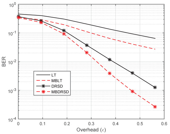
Figure 7.
Bit error rate (BER) versus the overhead () for different coding schemes at and erasure probabilities of , , and .
In order to show that the same enhancements are applicable in different environments, the DSP and BER for the same schemes with different channel environments are shown in Figure 8 and Figure 9, respectively. The new channel erasure rates are , , and . These two figures show that using the proposed scheme enhances the performance once it applies to the regular LT codes or DRSD. While the DSP and BER are improved, the decoding time is insignificantly increased. For example, with an overhead of , the regular LT code requires 1.6 ms, and it achieves BER = 0.1553, whereas the MBLT code requires 1.7 ms, and it achieves BER = 0.07836. Likewise, DRSD and MBDRSD require 1.73 ms and 1.87 ms, respectively, and they achieve a BER of 0.0105 and , respectively.
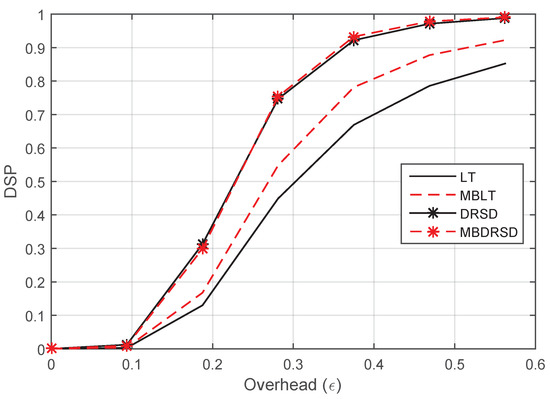
Figure 8.
DSP versus the overhead () for different coding schemes at and erasure probabilities of , , and .
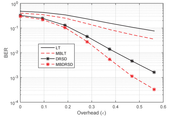
Figure 9.
BER versus the overhead () for different coding schemes at and erasure probabilities of , , and .
Moreover, Figure 10, Figure 11, Figure 12 and Figure 13 show the BER of the same schemes at a larger length of source symbols, , under many channels’ environments. For example, Figure 10 shows the BER in perfect channels between all nodes. We can see that the best algorithm is our proposed algorithm when it applies to the DRSD (i.e., MBDRSD). In addition, Figure 11 is depicted in a different scenario, where a perfect channel is between the relay and the destination (), whereas homogeneous channels are between each sender and the relay ( and ). Moreover, Figure 12 depicts a scenario in which all three channels have the same erasure probability (). Finally, Figure 13 is obtained when the erasure channel between the relay and the destination is , and the erasure channels between each sender and the relay are . As can be seen from the figures, the MBLT codes are superior to the regular LT codes. Moreover, similar improvements are obtained once the proposed scheme is applied to the DRSD.
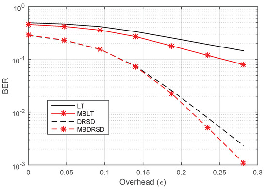
Figure 10.
BER versus the overhead () for different coding schemes at and erasure probabilities of , , and .
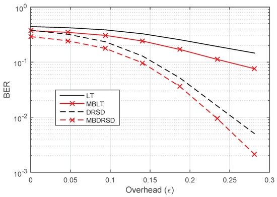
Figure 11.
BER versus the overhead () for different coding schemes at and erasure probabilities of , , and .
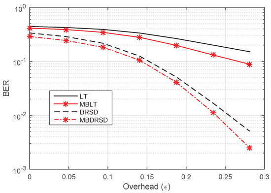
Figure 12.
BER versus the overhead () for different coding schemes at and erasure probabilities of , , and .
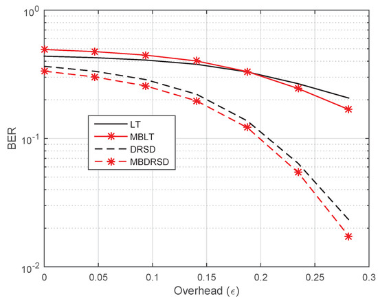
Figure 13.
BER versus the overhead () for different coding schemes at and erasure probabilities of , , and .
6. Conclusions
Designing efficient and robust communications is indispensable for 5G and 6G networks, where many requirements, such as low latency, high reliability, low complexity, and flexibility, must be fulfilled. These requirements can be fulfilled by using the fountain codes [32]. This paper proposes using a modified version of the fountain codes (i.e., LT codes) over the Y-network. Then, we optimize the LT codes’ parameters to maximize the decoding success probability (DSP). Furthermore, we propose an efficient encoding scheme using a memory-based strategy to enhance the performance of the Y-network. Finally, simulation results show that the proposed scheme consistently outperforms traditional LT code schemes with respect to the DSP, BER, complexity, and delay. In fact, the proposed scheme framework can be efficiently adapted to any work with other encoding processes in the literature. With this intention, we adapt our proposed scheme to one of the state-of-the-art encoding processes, decreasing ripple size distribution (DRSD), and compare the results. Likewise, the proposed scheme outperforms the DRSD in terms of the DSP and BER. For instance, for a code length and a number of transmitted symbols , and when all the three channels in the Y-network are perfect, our results show that the proposed scheme achieves significant improvements compared with regular LT codes as well as DRSD codes.
Funding
This research received no external funding.
Conflicts of Interest
The author declares no conflict of interest.
References
- Hale, J. More than 500 Hours of Content Are Now Being Uploaded to YouTube Every Minute. Available online: https://www.tubefilter.com/2019/05/07/number-hours-video-uploaded-to-youtube-per-minute/ (accessed on 25 October 2021).
- Hsieh, P.J.; Lin, W.S.; Lin, K.H.; Wei, H.Y. Dual-Connectivity Prevenient Handover Scheme in Control/User-Plane Split Networks. IEEE Trans. Veh. Technol. 2018, 67, 3545–3560. [Google Scholar] [CrossRef]
- Demarchou, E.; Psomas, C.; Krikidis, I. Mobility management in ultra-dense networks: Handover skipping techniques. IEEE Access 2018, 6, 11921–11930. [Google Scholar] [CrossRef]
- Mumtaz, T.; Muhammad, S.; Aslam, M.I.; Mohammad, N. Dual connectivity-based mobility management and data split mechanism in 4G/5G cellular networks. IEEE Access 2020, 8, 86495–86509. [Google Scholar] [CrossRef]
- Gures, E.; Shayea, I.; Alhammadi, A.; Ergen, M.; Mohamad, H. A comprehensive survey on mobility management in 5G heterogeneous networks: Architectures, challenges and solutions. IEEE Access 2020, 8, 195883–195913. [Google Scholar] [CrossRef]
- Shayea, I.; Ergen, M.; Azmi, M.H.; Çolak, S.A.; Nordin, R.; Daradkeh, Y.I. Key challenges, drivers and solutions for mobility management in 5G networks: A survey. IEEE Access 2020, 8, 172534–172552. [Google Scholar] [CrossRef]
- Liau, A.; Yousefi, S.; Kim, I.M. Binary soliton-like rateless coding for the Y-network. IEEE Trans. Commun. 2011, 59, 3217–3222. [Google Scholar] [CrossRef]
- Byers, J.W.; Luby, M.; Mitzenmacher, M.; Rege, A. A digital fountain approach to reliable distribution of bulk data. ACM SIGCOMM Comput. Commun. Rev. 1998, 28, 56–67. [Google Scholar] [CrossRef]
- Luby, M. LT codes. In Proceedings of the 43rd Annual IEEE Symposium on Foundations of Computer Science, Vancouver, BC, Canada, 16–19 November 2002; pp. 271–280. [Google Scholar]
- Etesami, O.; Shokrollahi, A. Raptor codes on binary memoryless symmetric channels. IEEE Trans. Inf. Theory 2006, 52, 2033–2051. [Google Scholar] [CrossRef]
- Hayajneh, K.F.; Yousefi, S.; Valipour, M. Left degree distribution shaping for LT codes over the binary erasure channel. In Proceedings of the 27th Biennial Symposium on Communications (QBSC), Kingston, ON, Canada, 1–3 June 2014; pp. 198–202. [Google Scholar]
- Hayajneh, K.F.; Yousefi, S. Robust LT designs in binary erasures. In Proceedings of the 15th Canadian Workshop on Information Theory (CWIT), Quebec City, QC, Canada, 11–14 June 2017; pp. 1–5. [Google Scholar]
- Xu, S.; Xu, D. Optimization design and asymptotic analysis of systematic Luby transform codes over BIAWGN channels. IEEE Trans. Commun. 2016, 64, 3160–3168. [Google Scholar] [CrossRef]
- Song, X.; Cheng, N.; Liao, Y.; Ni, S.; Lei, T. Design and Analysis of LT Codes with a Reverse Coding Framework. IEEE Access 2021, 9, 116552–116563. [Google Scholar] [CrossRef]
- Hayajneh, K.F.; Yousefi, S. Improved systematic fountain codes in AWGN channel. In Proceedings of the 13th Canadian Workshop on Information Theory, Toronto, ON, Canada, 18–21 June 2013; pp. 148–152. [Google Scholar]
- Castura, J.; Mao, Y. Rateless coding over fading channels. IEEE Commun. Lett. 2006, 10, 46–48. [Google Scholar] [CrossRef]
- Liu, X.; Lim, T.J. Fountain codes over fading relay channels. IEEE Trans. Wirel. Commun. 2009, 8, 3278–3287. [Google Scholar] [CrossRef]
- Shokrollahi, A. Raptor codes. IEEE Trans. Inf. Theory 2006, 52, 2551–2567. [Google Scholar] [CrossRef]
- Hayajneh, K.F.; Yousefi, S.; Valipour, M. Improved finite-length Luby-transform codes in the binary erasure channel. IET Commun. 2015, 9, 1122–1130. [Google Scholar] [CrossRef]
- Puducheri, S.; Kliewer, J.; Fuja, T.E. Distributed LT codes. In Proceedings of the 2006 IEEE International Symposium on Information Theory, Seattle, WA, USA, 9–14 July 2006; pp. 987–991. [Google Scholar]
- Puducheri, S.; Kliewer, J.; Fuja, T.E. The design and performance of distributed LT codes. IEEE Trans. Inf. Theory 2007, 53, 3740–3754. [Google Scholar] [CrossRef] [Green Version]
- Sejdinovic, D.; Piechocki, R.J.; Doufexi, A. AND-OR tree analysis of distributed LT codes. In Proceedings of the 2009 IEEE Information Theory Workshop on Networking and Information Theory, Volos, Greece, 10–12 June 2009; pp. 261–265. [Google Scholar]
- Liau, A.; Kim, I.M.; Yousefi, S. Improved low-complexity soliton-like network coding for a resource-limited relay. IEEE Trans. Commun. 2013, 61, 3327–3335. [Google Scholar] [CrossRef]
- Zhang, L.; Su, L. Goal-oriented design of optimal degree distribution for LT codes. IET Commun. 2020, 14, 2658–2665. [Google Scholar] [CrossRef]
- Hussain, I.; Xiao, M.; Rasmussen, L.K. Buffer-based distributed LT codes. IEEE Trans. Commun. 2014, 62, 3725–3739. [Google Scholar] [CrossRef]
- Cheng, X.; Cao, R.; Yang, L. Stochastic Polynomial Decomposition-Based Energy-Efficient Hybrid DLT Codes. IEEE Trans. Commun. 2016, 64, 4897–4909. [Google Scholar] [CrossRef]
- He, J.; Hussain, I.; Li, Y.; Juntti, M.; Matsumoto, T. Distributed LT codes with improved error floor performance. IEEE Access 2019, 7, 8102–8110. [Google Scholar] [CrossRef]
- Luby, M.G.; Mitzenmacher, M.; Shokrollahi, M.A.; Spielman, D.A. Efficient erasure correcting codes. IEEE Trans. Inf. Theory 2001, 47, 569–584. [Google Scholar] [CrossRef] [Green Version]
- Lu, H.; Lu, F.; Cai, J.; Foh, C.H. LT-W: Improving LT decoding with Wiedemann solver. IEEE Trans. Inf. Theory 2013, 59, 7887–7897. [Google Scholar] [CrossRef]
- Karp, R.; Luby, M.; Shokrollahi, A. Finite length analysis of LT codes. In Proceedings of the International Symposium onInformation Theory (ISIT 2004), Chicago, IL, USA, 27 June–2 July 2004; p. 39. [Google Scholar]
- Sorensen, J.H.; Popovski, P.; Ostergaard, J. Design and Analysis of LT Codes with Decreasing Ripple Size. IEEE Trans. Commun. 2012, 60, 3191–3197. [Google Scholar] [CrossRef]
- Abbas, R.; Shirvanimoghaddam, M.; Huang, T.; Li, Y.; Vucetic, B. Novel design for short analog fountain codes. IEEE Commun. Lett. 2019, 23, 1306–1309. [Google Scholar] [CrossRef]
Publisher’s Note: MDPI stays neutral with regard to jurisdictional claims in published maps and institutional affiliations. |
© 2021 by the author. Licensee MDPI, Basel, Switzerland. This article is an open access article distributed under the terms and conditions of the Creative Commons Attribution (CC BY) license (https://creativecommons.org/licenses/by/4.0/).