Deep Learning and Machine Learning Techniques of Diagnosis Dermoscopy Images for Early Detection of Skin Diseases

Abstract

With the increasing incidence of severe skin diseases, such as skin cancer, endoscopic medical imaging has become urgent for revealing the internal and hidden tissues under the skin. Diagnostic information to help doctors make an accurate diagnosis is provided by endoscopy devices. Nonetheless, most skin diseases have similar features, which make it challenging for dermatologists to diagnose patients accurately. Therefore, machine and deep learning techniques can have a critical role in diagnosing dermatoscopy images and in the accurate early detection of skin diseases. In this study, systems for the early detection of skin lesions were developed. The performance of the machine learning and deep learning was evaluated on two datasets (e.g., the International Skin Imaging Collaboration (ISIC 2018) and Pedro Hispano (PH2)). First, the proposed system was based on hybrid features that were extracted by three algorithms: local binary pattern (LBP), gray level co-occurrence matrix (GLCM), and wavelet transform (DWT). Such features were then integrated into a feature vector and classified using artificial neural network (ANN) and feedforward neural network (FFNN) classifiers. The FFNN and ANN classifiers achieved superior results compared to the other methods. Accuracy rates of 95.24% for diagnosing the ISIC 2018 dataset and 97.91% for diagnosing the PH2 dataset were achieved using the FFNN algorithm. Second, convolutional neural networks (CNNs) (e.g., ResNet-50 and AlexNet models) were applied to diagnose skin diseases using the transfer learning method. It was found that the ResNet-50 model fared better than AlexNet. Accuracy rates of 90% for diagnosing the ISIC 2018 dataset and 95.8% for the PH2 dataset were reached using the ResNet-50 model.

1. Introduction

The skin is the largest human organ, and it is the outer covering of the body. The skin is the first line of defense in the human body [1]. It has the role of (i) protecting the internal organs from external environmental influences, (ii) regulating body temperatures, (iii) providing immunity against many diseases, and (iv) providing beauty to the body [2]. The human body is protected by the skin from harmful ultraviolet rays from the sun, although the essential vitamin D is also produced by this organ when the body is exposed to sunlight. Skin color (body pigmentation) and moisture (from oily to dry skin) vary from person to person according to the hot and cold regions in the world [3]. Cellular DNA is damaged if the body is exposed to sunlight or ultraviolet rays for a long time, decreasing skin pigmentation and the incidence of malignant skin diseases. Skin cancer (melanoma) is a fatal skin disease with no early diagnosis. In the early stages of the disease, it is not detected due to the similarity of the cancer cells to other skin cells. Abnormal cancerous cells divide rapidly, penetrating the lower skin layers and becoming incurable malignant melanomas [4].

Disease treatment is challenging when melanoma cells spread throughout the body. Therefore, early diagnosis is required to save lives. According to dermoscopy images, there are many types of skin diseases. The two main types of skin disease can be identified as melanocytic and nonmelanocytic. Melanocytic diseases have two types: melanoma and melanocytic nevi [5,6]. In contrast, nonmelanocytic skin diseases contain five types: basal cell carcinoma (BCC), squamous cell carcinoma (SCC), vascular (VASC), benign keratosis lesions (BKL), and dermatofibroma (df). Melanoma (mel) is one of the most dangerous and deadly skin diseases. It is incurable in its late stages and is one of the most common cancers worldwide.

There are many challenges, including different skin colors from one person to another and artifacts, hair, and air bubbles. In addition, there are many similar features between types of skin diseases, especially in the early stages. More than 420 million people are suffering from skin diseases worldwide, representing a limitation in terms of insufficient medical resources. Furthermore, the high treatment cost represents a challenge, especially in developing countries, which causes delays in early diagnosis and leads to the deterioration of life and social development [7].

According to the American Cancer Society (ACS), there were more than 70,000 cases in the United States in 2017. In 2020, 100,350 cases of melanoma were diagnosed in that country, with 60,190 cases occurring in men and 40,160 occurring in women [8]. Because of lesion’s early-stage similarity, experts and clinicians find distinguishing melanoma and benign early-stage lesions difficult. Therefore, early diagnosis using computer-aided diagnostic techniques (e.g., artificial intelligence) has become essential. Computer-aided diagnosis is critical to helping physicians and experts save time and effort during early disease diagnosis. In our research, we used artificial intelligence techniques for the early diagnosis of skin lesions. With many layers and complex neurons, specific samples are trained using artificial intelligence techniques to solve particular problems. Deep learning techniques have been used to solve complex diagnostic problems that can hardly be solved using machine learning techniques [9].

Artificial intelligence techniques have been applied to classify many types of images and medical records, such as dermatoscopy, magnetic resonance imaging, computed tomography (CT) scans, and medical records [10,11]. Artificial intelligence techniques have been used to improve the quality of the entered images by using pre-processing methods, identifying lesion areas, and isolating them from healthy skin to focus on the disease area. Then, essential features (e.g., shape, texture, color, and shape) from each image are extracted and distinguished from other images in which these features are stored. Finally, the features are fed into the classification stage to diagnose each lesion in the appropriate class.

The main contributions of this study are as follows:

• Extract the important features from each image with LBP, GLCM, and DWT algorithms, combining the extracted features into one vector to obtain representative features for each image; diagnose the images using artificial neural networks ANN and FFNN classifiers.
• The capabilities of deep learning networks lie in imparting acquired skills to solve new, relevant problems.
• In this research, the early diagnosis of skin lesions and distinguishing benign images from malignant ones are considered.
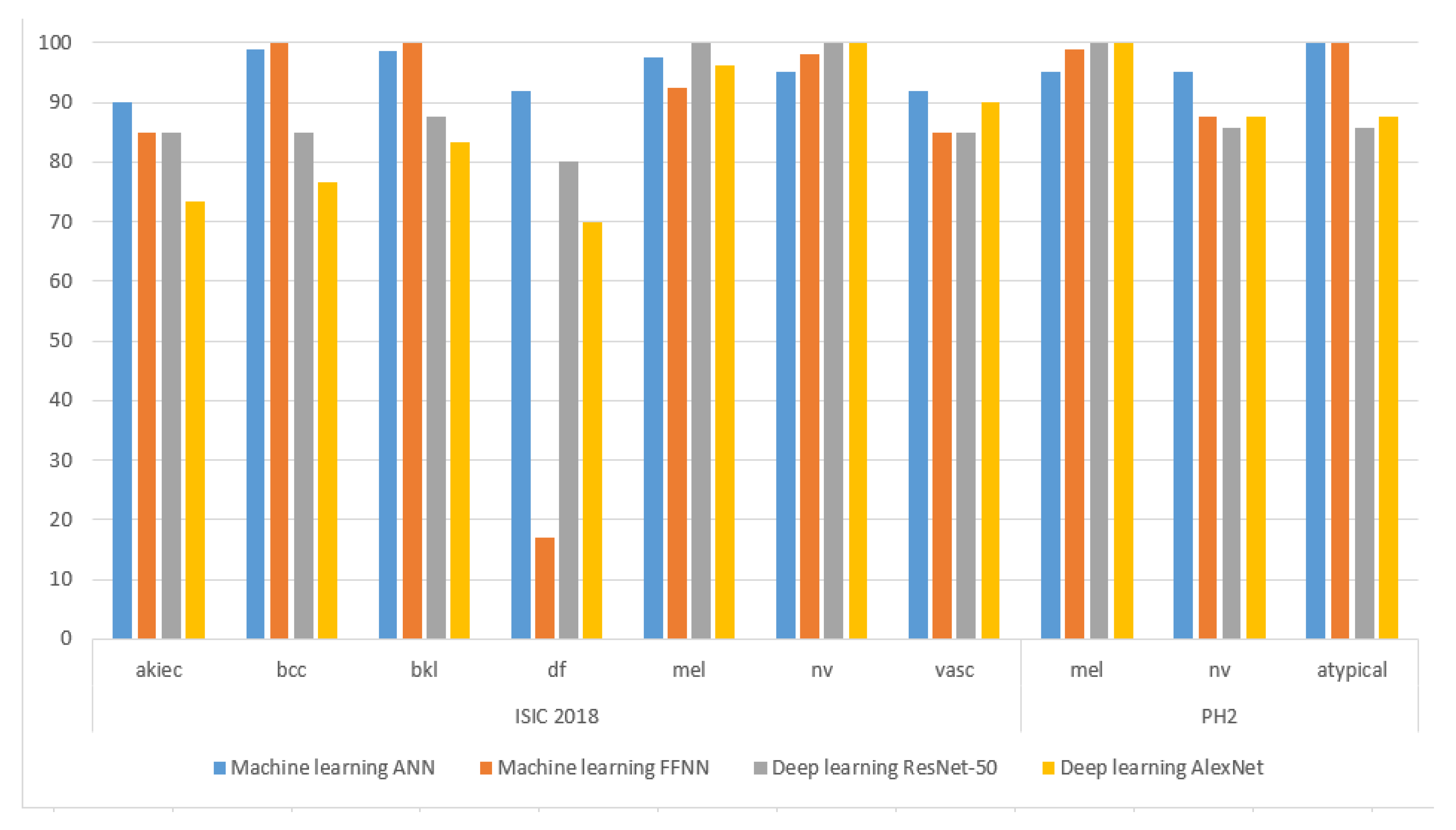
• Machine learning algorithms (ANN and FFNN) achieved better results than CNN models (ResNet-50 and AlexNet).
• Machine and deep learning techniques will help medical doctors in the early detection of skin lesions, enhancing the confidence of doctors and reducing the number of biopsies and surgeries.

The remainder of the manuscript is organized as follows: related work is discussed in Section 2. In Section 3, the analysis of materials and methodology, containing subsections of image processing methods, is discussed. Later, the results achieved by machine learning algorithms and deep learning are described and compared in Section 4. Then, the discussion of the research is summarized in Section 5. Finally, in Section 6, conclusions regarding this manuscript are provided.

2. Related Work

Many researchers from interested scientific communities have worked on diagnosing skin lesions using artificial intelligence techniques in recent years. Qin et al. (2020) discussed generative adversarial networks (GANs), where a generator and discriminator would be tuned by the network to produce high-resolution images and remove noise. The network evaluation was conducted through a set of images produced by the GANs, and the network achieved high performance [12]. Tschandl et al. (2019) retrained the ResNet-34 model on the skin lesion dataset through ImageNet and fine-tuned the ResNet-34 Jaccard system through ImageNet, achieving the highest random tuning [13].

Sreelatha et al. (2019) discussed the gradient and feature adaptive contour (GFAC) method for lesion zone segmentation and early detection of melanoma [14]. Chatterjee et al. (2019) proposed a recursive feature elimination (RFE) method based on multilayer images. Color, texture, and shape features were extracted by GLCM and fractal-based regional texture analysis (FRTA) methods and feature classification by the support vector machine (SVM) algorithm [15]. Al-Masni et al. (2020) proposed a technique that combines both lesion segmentation and classification. First, a full-resolution convolutional network (FrCN) was used to segment the melanoma. Then, deep learning models were used to categorize segmented lesions [16]. Alzubaidi et al. (2021) proposed a new approach for transferring learning to train an extensive ISIC dataset and transfer knowledge to a target dermatology dataset. Furthermore, CNNs, in which recent developments are combined, were used to diagnose skin lesions with high accuracy [17].

Liu et al. (2021) proposed a multiscale ensemble of convolutional neural networks (MECNN), which consists of three branches. In the first branch, the lesion area is defined by selecting the most points around the lesion. Then, the search area of a region of interest is reduced using the MECNN method. Finally, the outline was divided into two inputs for the other two branches [18]. Ding et al. (2021) proposed conditional GANs (CGANs) to obtain high-resolution images. The segmentation mask and class labels were combined to establish an efficient mapping of the pathological markers of interest in that study. Translation from an image to a matrix is performed in CGAN methods. Then, such a matrix is assigned to a label as an input for each image [19]. Surówka et al. (2021) proposed the wavelet packet method for feature extraction through four wavelet decomposition channels. The features are classified by a logistic classifier that can extract high-resolution wavelet properties [20]. Iqbal et al. (2021) proposed a carefully designed deep convolutional neural network model with multiple layers and various filter sizes [21].

Sikkandar et al. (2021) proposed a diagnostic model based on lesion segmentation using the GrabCut method and the adaptive neuro-fuzzy classifier [22]. Ali et al. (2021) introduced the DCNN model, in which noise and artifacts were first removed from the images. In this method, image normalization and deep feature extraction are performed. Then data augmentation during the training phase was applied for the model to acquire a large number of images [23]. Kim et al. (2021) proposed a hair removal method from the lesion area on the image itself. Thus, coarse hair is removed by the algorithm while preserving the features of the lesion [24].

Tyagi et al. (2020) proposed an intelligent prognostic model for disease prediction and classification using a combination of CNN with particle swarm optimization (PSO) [25]. Ahmad et al. (2021) discussed the generative adversarial networks (GANs) method for training a convolutional neural network on a balanced dataset [26]. Molina-Molina et al. (2020) proposed a 1D fractal signature method for extracting texture features and combining them with features extracted using the Densenet-201 model. Such features would then be used as feature vectors to both classifiers K-nearest neighbors and SVM for diagnosing skin lesions [27]. Adegun et al. (2020) proposed a framework for the segmentation and classification of skin lesions. This method consists of two stages. In the first stage of the encoder-decoder fully convolutional network, complex and heterogeneous features are learned. In the second stage, the coarse texture is extracted at the encoder stage, and the lesion boundaries are extracted during the decoding stage [28].

Khan et al. (2021) presented a High-Frequency approach with a Multilayered Feed-Forward Neural Network (HFaFFNN) to integrate all images, enhance images with a log-opening-based activation function. Pre-trained CNNs Darknet-53 and NasNet-mobile have been implemented, and parameters are tuned for high performance. Finally, a parallel max entropy correlation (PMEC) algorithm was used to fuse the extracted features [29]. Muhammad et al. (2021) presented a two-stage framework for segmentation and classification. For lesions segmentation, a hybrid technique was used through the complementary strengths of two CNNs to produce a region of interest (RoI). To classify lesions by CNNs, 30 layers were trained on the HAM10000 dataset. The most important features were selected using the Regular Falsi method; the system achieved a good performance in diagnosing skin lesions [30]. Muhammad et al. (2021) presented a two-way CNN information fusion framework for diagnosing melanoma. Image contrast was improved based on fusion, then improved features were extracted by the skewness-controlled moth-flame optimization method. The second frame uses the MobileNetV2 model to extract the features. Finally, the features extracted from the two methods are fused by the new parallel multimax coefficient correlation algorithm. The system achieved superior performance in diagnosing skin cancer [31]. Muhammad et al. (2021) presented a robust system for diagnosing skin lesions through several stages. Firstly, image enhancement using local color-controlled histogram intensity values (LCcHIV). Secondly, pest segmentation by novel Deep Saliency. The threshold function is applied to obtain binary images. Thirdly, the most important features were extracted through the improved moth flame optimization (IMFO) algorithm. Finally, the system achieved high performance in diagnosing skin lesions by incorporating features and categorizing them using the Kernel Extreme Learning Machine [32].

Previous studies contain many challenges such as hair, air bubbles, artifacts, and light reflections. Researchers also face challenges such as the similarity of characteristics between types of diseases, which constitute a major challenge in the diagnosis and distinction between diseases. Therefore, the proposed systems in this study addressed all the challenges of the previous studies. Many enhancement techniques improved the images by removing artifacts, air bubbles, skin lines, and reflections by applying two filters together, namely Laplacian and average filters. Furthermore, the Dullrazor technology works with images containing hair and removes hair with high accuracy. As for the challenges of similar features between some diseases, three hybrid algorithms were applied to extract the features from each image and combine the features extracted from the three methods into one vector for each image. Thus, each disease is represented by its representative features. Parameters and weights of two models, ResNet-50 and AlexNet, were also adjusted to extract each disease’s deep and representative characteristics.

3. Materials and Methodology

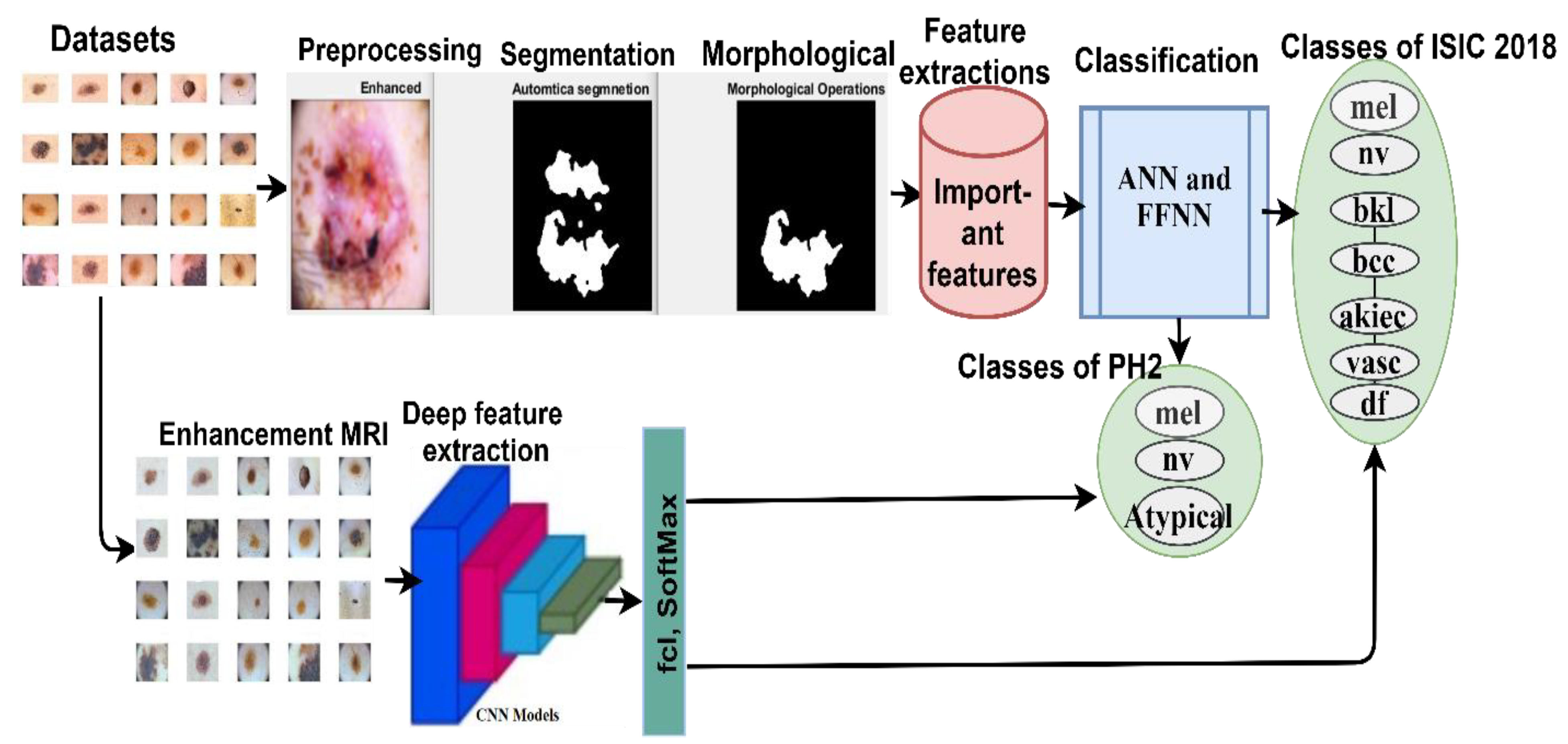
The evaluated proposed systems were applied to two datasets: ISIC 2018 and PH2. Each of these datasets was collected under different conditions and had different characteristics. The use of each dataset has several inherent challenges. The most important of which are (i) isolating the lesion from healthy skin (segmentation), (ii) localizing the features and patterns, (iii) and extracting and classifying the features of each lesion. Therefore, skin lesions may be detected by the systems, and skin cancer may be distinguished from other kinds of lesions. In Figure 1, the mechanism of action of the proposed method for diagnosing skin diseases is described. Images were enhanced, and the noise was removed using Laplacian and average filters and hair removal with the Dullrazor technique. The lesion segmentation was performed using the adopted region growth algorithm. Feature extraction was conducted in two different ways, in which traditional and deep learning were considered. In traditional methods, features were extracted by combining the extracted features through three algorithms: LBP, GLCM, and DWT. The deep feature maps were also extracted by CNN for the ResNet-50 and AlexNet models. The features extracted using traditional methods were classified using ANN and FFNN. At the same time, the deep feature maps were classified by two pre-trained CNNs, namely ResNet-50 and AlexNet models.

3.1. Dataset

In this study, the two standard datasets, namely, ISIC 2018 and PH2, were used for diagnosing dermatological diseases, which are explained as follows.

3.1.1. International Skin Imaging Collaboration (ISIC 2018) Dataset

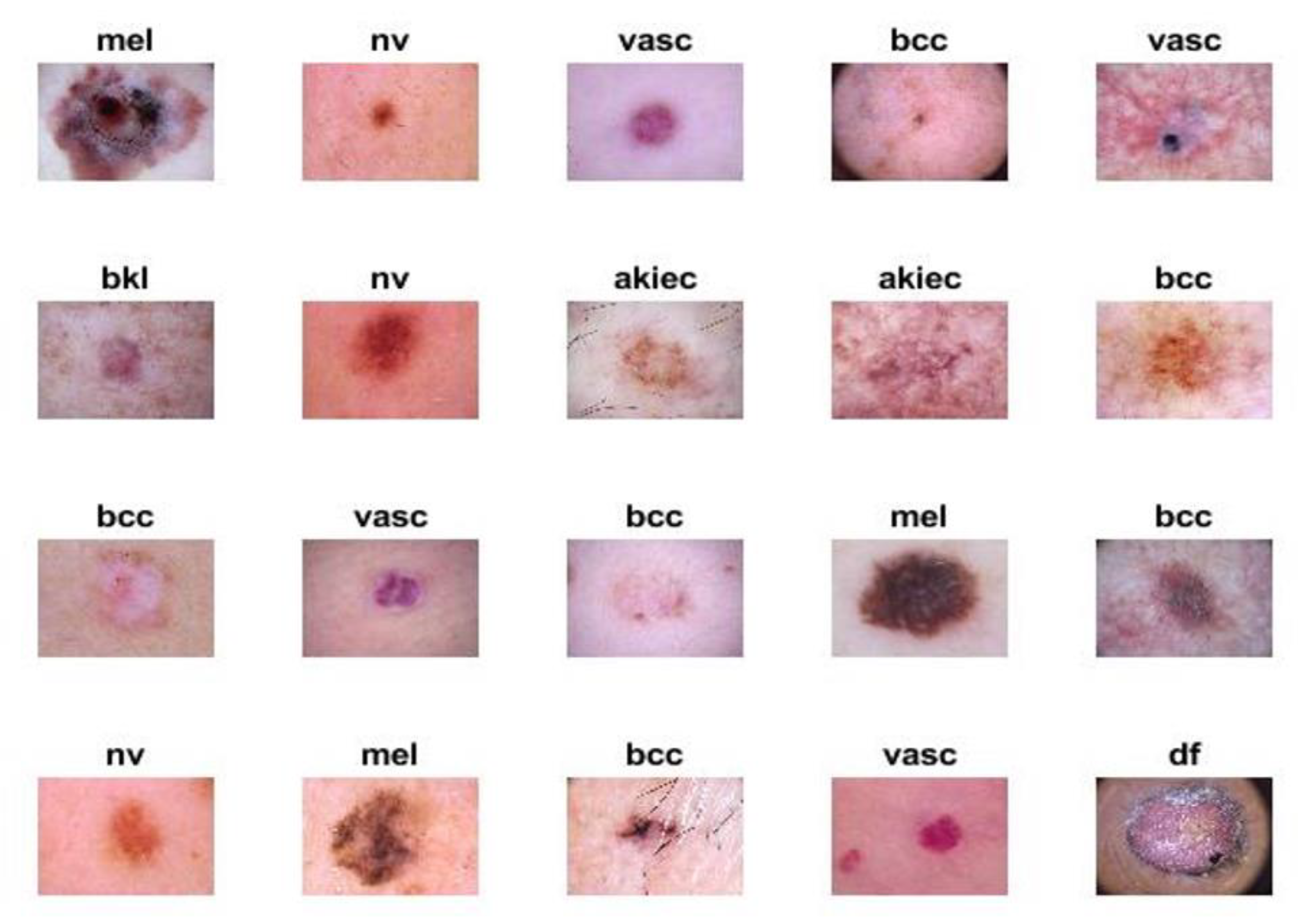
The proposed systems were evaluated using the ISIC 2018 dataset. The criteria for endoscopic devices were assessed to obtain high-resolution images and techniques, such as illumination, size, calibration markers, poses, magnification, terminology as diagnoses, lesion site, and morphology. The ISIC 2018 dataset, also known as HAM-10000, contains seven unbalanced diseases. In this study, the different kinds of diseases evaluated from this dataset and the amount of images considered in each condition were the following: actinic keratoses (AKIEC; n = 200 images), basal cell carcinoma (BCC; n = 200 images), benign keratosis lesions (BKL; n = 200 images), dermatoma (DF; n = 100 images), melanoma (MEL; n = 200 images), melanocytic nevi (NV; n = 200 images), and vascular (VASC; n = 100 images). In Figure 2, the samples from the ISIC 2018 dataset for seven diseases are described. The data from ISIC 2018 used in this study may be obtained [33].

3.1.2. PH2 Dataset

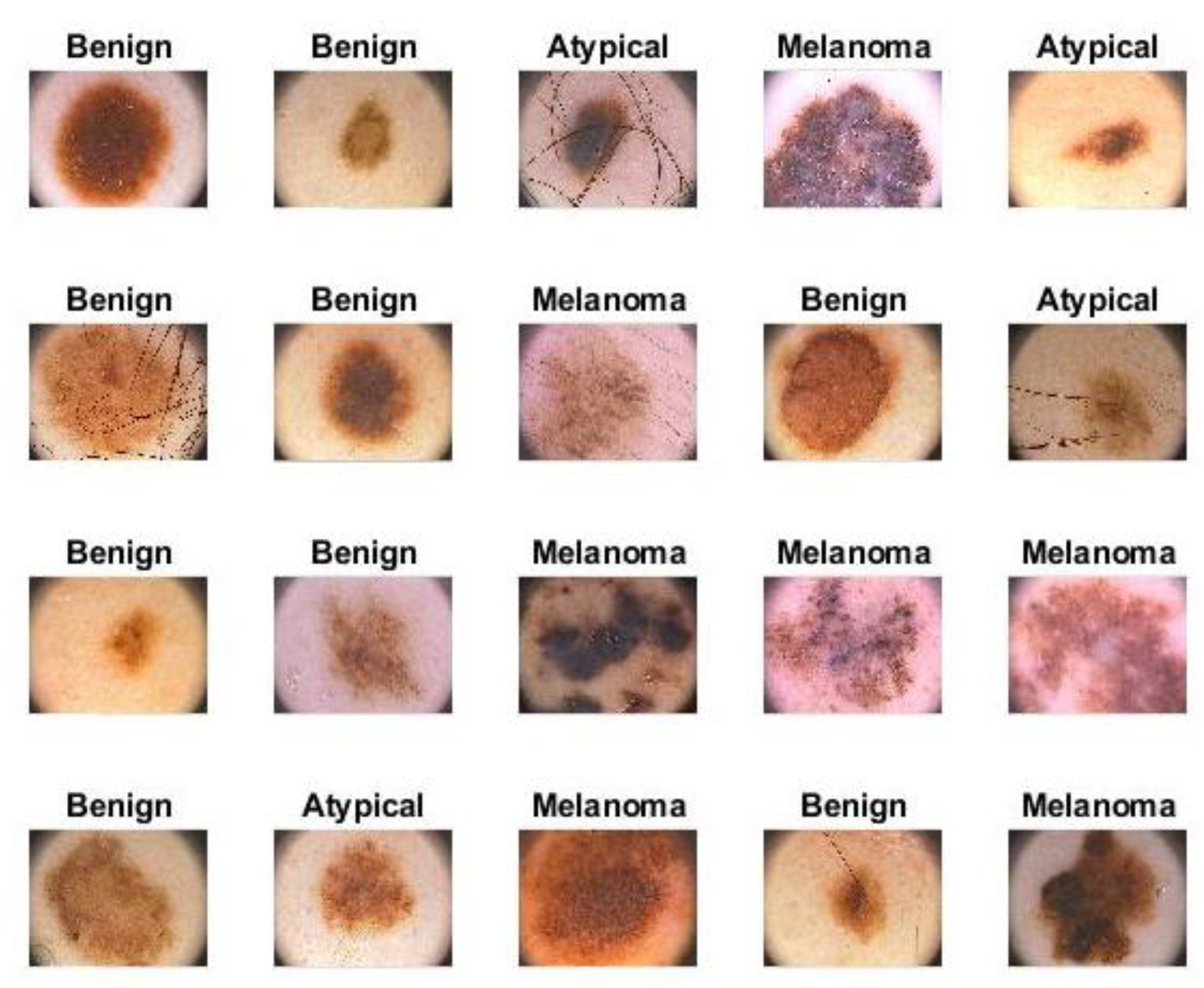
The proposed systems were evaluated on the PH2 dataset obtained from the Dermatology Service of Hospital Pedro Hispano (Matosinhos, Portugal). All images were obtained under the same conditions and instrumentation resolution. The dataset consisted of 200 images divided into three diseases: melanocytic nevi (NV; n = 80 images), atypical (n = 80 images), and melanoma (mel; n = 40 images). Where melanocytic nevi are benign tumors and melanoma is a malignant tumor, while atypical have characteristics of benign tumors but may develop into malignant tumors. In Figure 3, samples from the PH2 dataset are described. The data from the PH2 dataset used in this study may be obtained [34].

3.2. Pre-Processing

The pre-processing process is the first stage of image processing. In this section, the following information is provided: a description of the filters applied to enhance the images and the hair removal method from the images.

3.2.1. Laplacian and Average Filter Methods

Image enhancement is the first step in image processing. During this process, some noisy features such as hair, air bubbles, skin lines, and reflections due to lighting, etc., in the image are fixed to obtain a more precise image. In this study, Laplacian and average filters were used to remove noise and artifacts, enhance edges, and treat low contrast between lesions and healthy skin. First, an average filter was applied. The image was smoothed by the average filter with a reduction in the differences between adjacent pixels. The filter was applied to image frames of 5 × 5 pixels each time. The process continues until the entire image is covered. Then, the value of each pixel in the image was replaced with an average value based on the adjacent values. In Equation (1), the mechanism of action of the intermediate filter is described.

$$z\left(m\right)=\frac{1}{M}{\displaystyle \sum }_{i=0}^{M-1}y\left(m-1\right)$$

(1)

where z(m) is the input, y(m − 1) is the previous input, and M is the number in the average filter.

The Laplacian filter, which is an edge detection filter, was then used. This filter detects the changing areas in the image (e.g., edges of skin lesions). In Equation (2), the general functioning of the Laplacian filter is explained.

$$\nabla {}^{2}f=\frac{\partial {}^{2}f}{{\partial }^{2}x}+\frac{\partial {}^{2}f}{{\partial }^{2}y}$$

(2)

where f is a second-order differential equation and x, y represents the coordinates in a 2D matrix.

Finally, the image enhanced by the Laplacian filter is subtracted from the image enhanced by the averaging filter to obtain a more improved image.

3.2.2. Hair Removal Technique

Hair is one of the challenges in diagnosing skin lesions. DullRazor is a pre-processing technology that removes hair from the lesion area. The presence of hair in the lesion area causes confusion for the segmentation methods, as well as the feature extraction algorithm, and the presence of hair causes the feature extraction algorithms to add some features of hair in addition to the features of the lesion; therefore, the resulting features will be inaccurate because they contain the features of both the lesion and the hair. Therefore, the DullRazor technique removes hair before the process of segmentation and extraction of features [35]. The following three steps were necessary for hair removal:

• The location of dark hair is determined by the process of morphological closing of the images of the two datasets that contain hair;
• The structure of long or thin hair is checked using bilinear interpolation and substitution of specified pixel values;
• The new pixels are then smoothed by a medium filter.

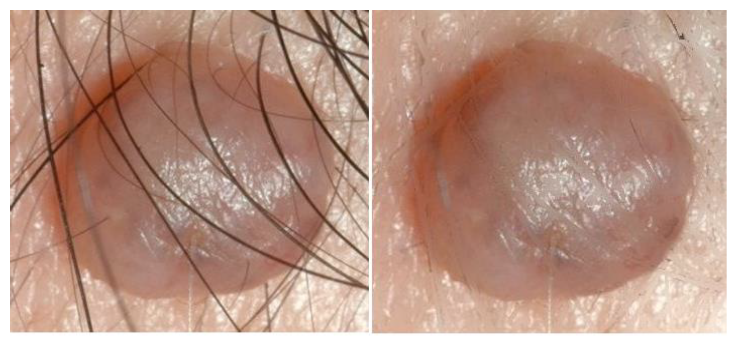
In Figure 4, a sample of the dataset images containing hair is shown. After applying the Dullrazor tool, the image was processed, and the hair was removed.

3.3. Adopted Region Growth Algorithm (Segmentation)

Dermatoscopy images consisted of an affected portion (skin lesion) and a healthy portion. Therefore, extracting features from the entire image, including healthy skin, leads to incorrect classification results [36]. Consequently, it is necessary to isolate the lesion region from normal skin. In this study, we used the adopted region growth algorithm. Groups of similar pixels were treated with this algorithm. The following conditions are needed for the successful segmentation process by the algorithm:

$${{\displaystyle \bigcup }}_{i=1}^m{y}_i=y,\mathrm{where}m\mathrm{is}\mathrm{the}\mathrm{number}\mathrm{of}\mathrm{regions}$$

$$y=1,2,\dots \dots ,Misconnected$$

$$P\left(y_i\right)=TRUEfor1,2,\dots \dots ,M$$

$$P\left(y_i{\displaystyle \bigcup }{y}_j\right)FALSEfori\ne j,where{y}_{i}andyareneighboringregions$$

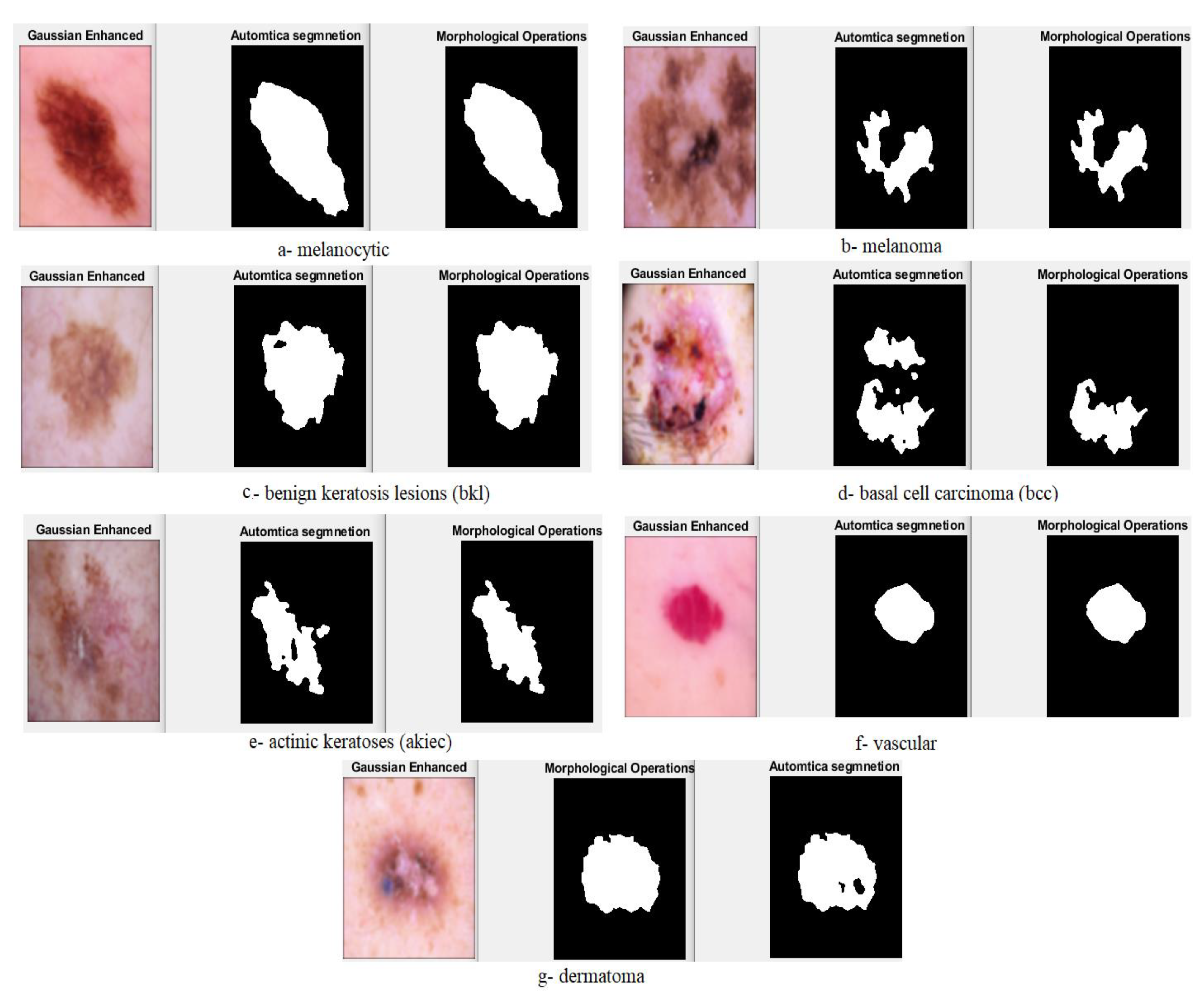
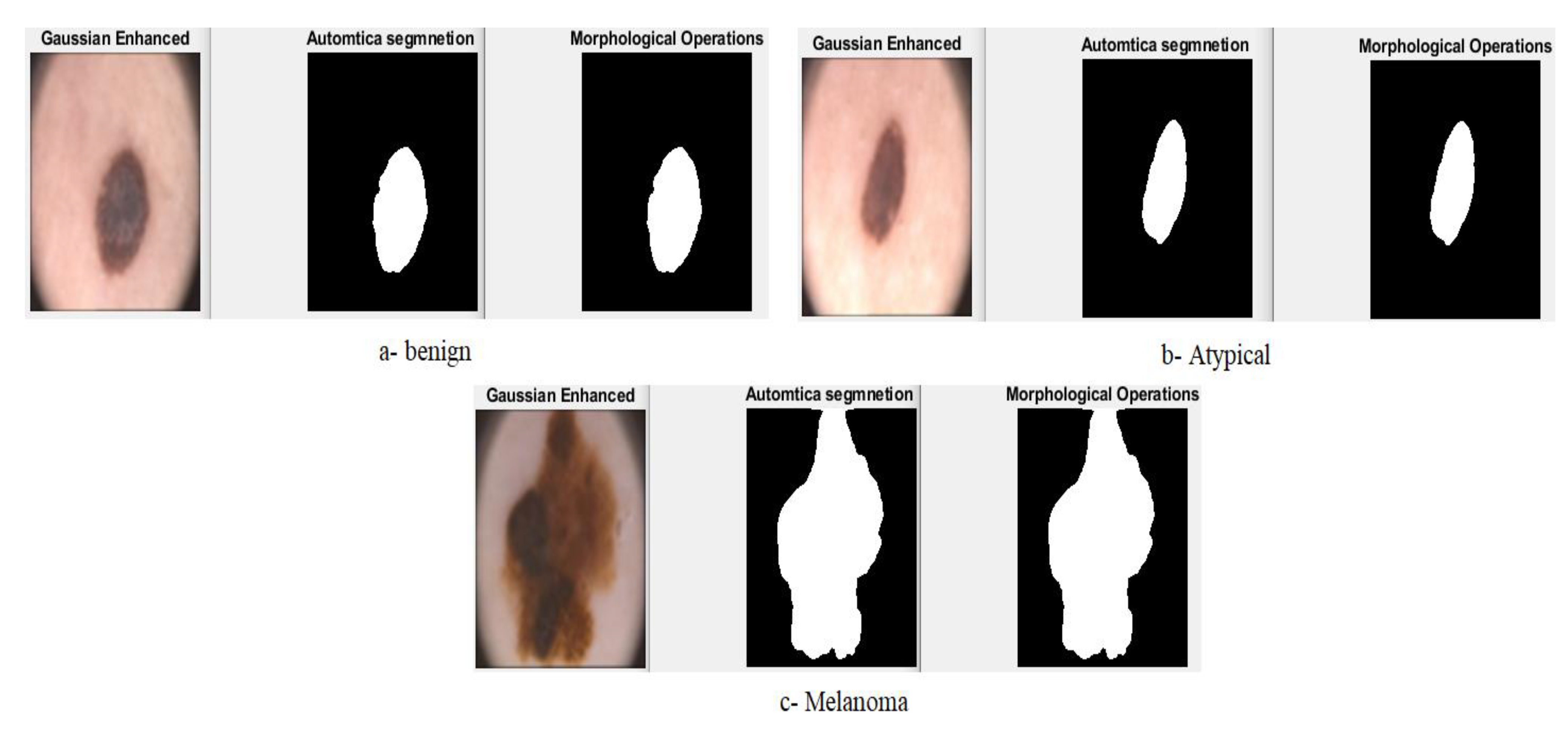
First, the segmentation process needs to be completed. Second, similar pixel units must be separated into different groups, and the union of all groups represents the whole image. Third, similar pixel units must be corrected. Fourth, no two pixels should be the same and belong to two different regions. The algorithm works on a bottom-up principle, where it starts from pixels and grows to form regions. Each region contains similar pixels. The basic idea is that the algorithm begins each region with a single-pixel seed. Then, each region grows with similar pixels, and the border regions grow with similar units to represent the boundaries of the lesion and separate it from healthy skin. In Figure 5 and Figure 6, samples from the ISIC 2018 and PH2 dataset are described, respectively. In these figures, the process is shown after the optimization, hair removal, segmentation process by isolating the lesion region from normal skin, and morphology method to further enhance the images, and the gaps of which were filled after the segmentation process.

3.4. Feature Extraction

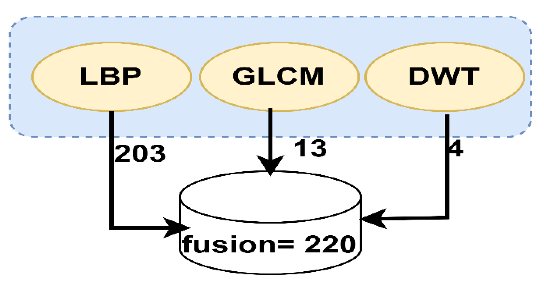
In this study, we combined three feature extraction methods, the LBP, GLCM, and DWT algorithms, to extract the most critical features of skin lesions from the images. The LBP algorithm is one of the simplest and most effective feature extraction algorithms. The central (target) pixel was determined using the algorithm. Then, a frame of 3 × 3 neighboring pixels was selected for each central pixel, known as the parameter R, representing the radius. This parameter was responsible for determining the number of adjacent pixels. Two-dimensional textures were described using the LBP algorithm [37]. In Equation (3), the decomposition of the center pixel by adjacent pixels is described, and the substitution of the resulting value of the center pixel. After this first step, the method continues for all pixels of the image. A total of 203 features were extracted for each image by the LBP algorithm.

$$LBP{\left(x_c,y_c\right)}_{R,P}={\displaystyle \sum }_{P=0}^{P-1}s\left((g_p-g_c\right)2^P$$

(3)

where g_c is the center pixel, g_p is the neighboring pixel, R is the radius around the central pixel, and P is the number of neighbors. The binary threshold function x is defined in Equation (4) as follows:

$$s\left(x\right)=\{\begin{array}{c}0, x<0\\ 1, x\ge 0\end{array}$$

(4)

The internal structure of the lesion area was displayed in gray levels using the GLCM algorithm. Then, the algorithm extracted texture features from an area of interest. Since the lesion area had a smooth and rough texture, the smooth area had pixel values close to each other, while the rough area had different pixels. Then, texture features from the spatial gray levels of a lesion were extracted using the algorithm. Textile metrics were calculated from spatial and statistical information. The location of a pixel from another pixel was determined by the spatial information in terms of a distance d and a direction θ. There were four values of θ: 0°, 45°, 90°, and 135°. Additionally, d = 1 when θ is horizontal or vertical (θ = 0° or θ = 90°), and d = √2 when θ (θ = 45° or θ = 135°). A total of 13 features was extracted for each image: contrast, energy, mean, entropy, correlation, kurtosis, standard deviation, smoothness, homogeneity, RMS, skewness, and variance.

Four features from each image were extracted using the DWT method, in which the input signal was analyzed into two signals with different frequencies using square mirror filters. These two signals were compatible with low-and high-pass filters. Approximation coefficients were produced by low-pass (LL) filters, while detailed coefficients (horizontal, vertical, and diagonal) were produced by high-pass filters (LH, HL, and HH). A total of 220 hybrid features were extracted using all the algorithms (LBP, GLCM and DWT). Such features were combined in one vector for each image. The produced vector was fed to the classification stage to train the classifier. In Figure 7, the hybrid process for feature extraction is described.

3.5. Classification

In this section, the ISIC 2018 and PH2 datasets were evaluated according to two traditional classification algorithms (e.g., ANN and FFNN) and convolutional neural networks (CNNs) (e.g., ResNet-50 and AlexNet) models for diagnosing skin diseases.

3.5.1. ANN and FFNN

ANN is a type of neural network of soft computing. It is a group of layers consisting of interconnected and internally connected neurons. It has a superior ability to interpret and analyze complex data and to produce clear and explanatory patterns. The error between actual and predicted probabilities is also minimized by ANN [38]. Information is propagated between neurons and stored as connecting points between them called weights. The objective of the ANN is to update the specified weights w to obtain the minimum square error between the actual output x and predicted output y as given by the mean square error (MSE), as described in Equation (5):

$$\mathrm{MSC}=\frac{1}{\mathrm{n}}{\displaystyle \sum }_{\mathrm{i}=1}^{\mathrm{n}}{\left(x_i-y_i\right)}^2$$

(5)

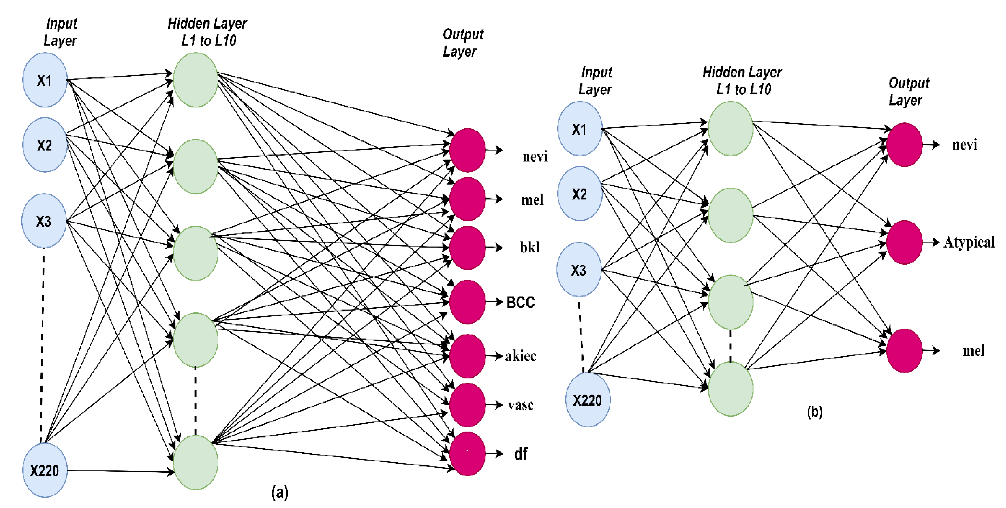
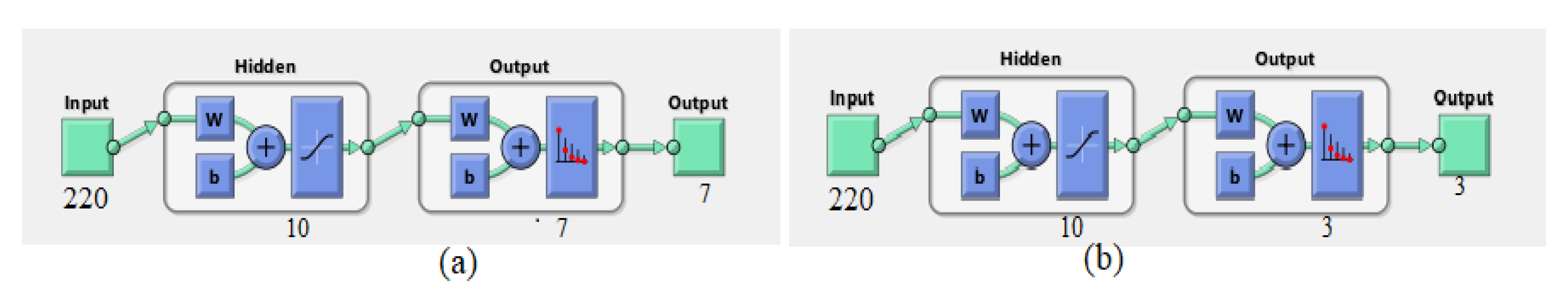
The ANN algorithm was evaluated on the ISIC 2018 and PH2 datasets for diagnosing skin diseases. A model was trained on 220 features through 10 hidden layers between the input and output layers. In Figure 8a, the architecture of the ANN algorithm is shown for the ISIC 2018 dataset. Seven classes were produced. In Figure 8b, the architecture of the ANN algorithm is shown for the PH2 dataset, in which three classes were produced.

The FFNN algorithm is similar to the ANN algorithm in solving complex computational problems. The hidden layer neurons are interconnected by w weights. The algorithm works, and information between neurons is fed in the forward direction. The results of each neuron were obtained based on the weight associated with it multiplied by the output of the previous neuron [39]. The weights were updated in the forward direction from the hidden layer to the output layer. In each iteration, the weights were updated until the minimum squared error was obtained between the expected and actual output. The criteria were used to select the algorithms ANN and FFNN. It is known that these algorithms are among the best machine learning algorithms and are distinguished from the rest of the machine learning algorithms by several criteria such as: (1) they contain many layers such as the input layer to receive the features (220 features in this study) and many layers of hidden (10 hidden layers in this study) and output layers (seven neurons in the case of the ISIC 2018 dataset or three neurons in the case of the PH2 dataset). (2) Interconnected neurons. (3) The weights that connect each neuron with the other neurons. (4) Mean square error compares the actual and predicted output and repeatedly works until the lowest ratio between the predicted and actual output is obtained by changing the weights frequently [40].

3.5.2. Convolutional Neural Networks (CNNs)

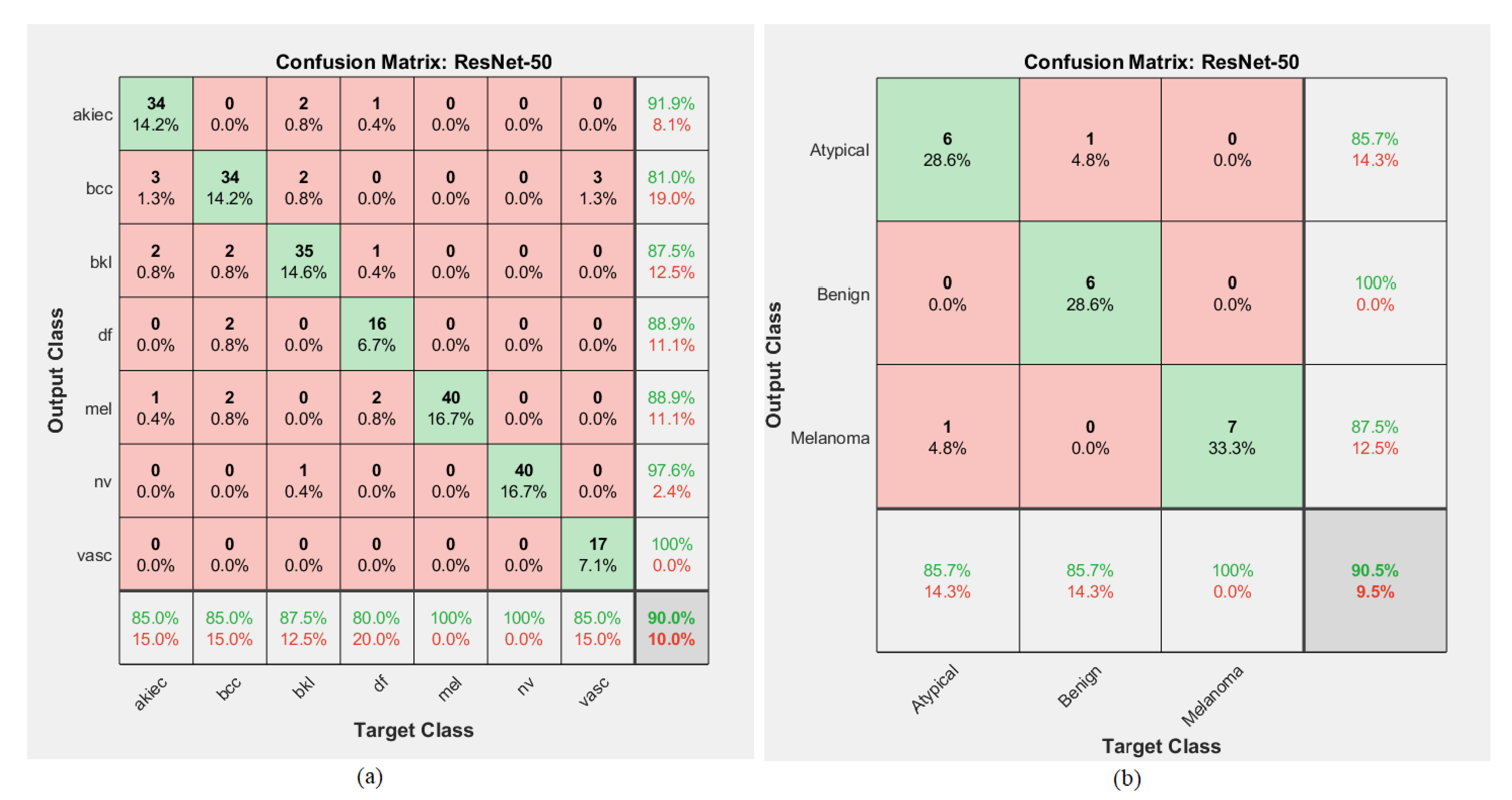
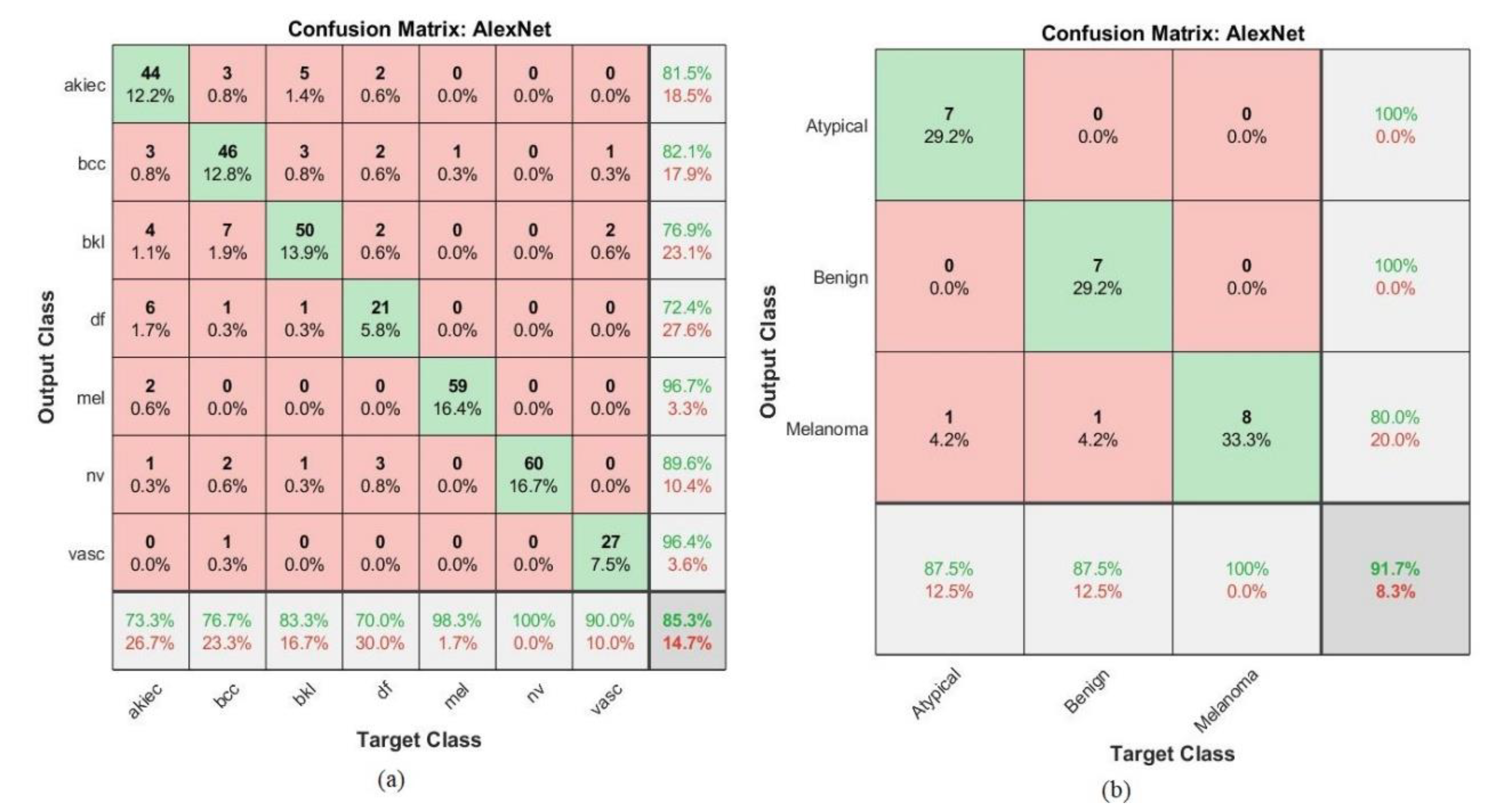
CNNs are deep learning methods used in many areas, including signal processing and image processing, to recognize patterns, classify objects, and detect regions of interest [41]. In this study, the two datasets, ISIC 2018 and PH2, were evaluated on ResNet-50 and AlexNet for diagnosing skin diseases. Several CNN structures for diagnosing skin lesions have been established, including several layers, training steps, activation functions, and learning rates. The most important layers in a CNN are the convolutional layers, max, average pooling layers, the fully connected layer, and activation functions [42].

When the image was inputted into the CNN structure, the image was represented as image height × image width. After the image passed through the convolutional layers, the feature map contained the feature depth, represented as image height × image width × image depth. Filter size, step, and zero padding were the most critical parameters of the convolutional layers that affected the performance of the convolutional layers. Convolutional layers wrap with the filter size around the image, learn the weights during the training phase, process the input, and pass it to the next layer.

Zero padding was the process of filling neurons with zeros to maintain the size of the resulting neurons. When zero padding was one, the neurons were padded with a row and a column around the edges. The output in each neuron was input to the next neuron. This output was calculated according to Equation (6) as follows:

$$OutputNeurons=\frac{W-K+2P}{S}+1$$

(6)

where W represents the volume of the input neuron, K represents the filter volume in a convolutional layer, P represents the volume of the input padding, and S represents the step. Rectified linear unit (ReLU) layers were also used after convolutional layers for image processing. The purpose of ReLU was to pass the positive output, suppress the negative output, and convert it to zero [43]. Equation (7) showns how a ReLU layer works.

$$\mathrm{ReLU}\left(\mathrm{x}\right)=\max \left(0,x\right)=\{\begin{array}{c}x, x\ge 0\\ 0, x<0\end{array}$$

(7)

The dimensions were reduced by the pooling layer, as the dimensions of the image were reduced by grouping many neurons and representing them in one neuron according to the maximum or average method, which is called the max-pooling layer or average pooling layer. The maximum value of the groups of neurons was selected using the maximum method, and the average value of the neurons was chosen using the average method. CNNs have millions of parameters, and there was an overfitting problem. Therefore, overfitting was prevented by the dropout layer by stopping 50% of the neurons, while the remaining neurons were turned on in each iteration. However, the training time was doubled by this technique due to repetition by an amount of two. In the fully connected layers, the last layer of convolutional neural networks, each neuron was connected to all neurons. Feature maps were converted to flat representations (unidirectional). Each image was diagnosed by a fully connected layer in its related class. Thus, the network takes a long time during the training and testing phases, and many fully connected layers can be used in the same network.

Softmax is the activation function used in the last stage of the convolutional neural network model. It is nonlinear and is used by multiple classes. In Equation (8), the functioning of the softmax function is described. Respectively, seven and three classes were produced for both the ISIC 2018 and PH2 datasets by the softmax function.

$$\begin{gathered} \mathrm{Output}0\le y\left(x\right)\le 1 \\ y\left(x_i\right)=\frac{\exp x_i}{{{\displaystyle \sum }}_{\mathrm{j}=1}^{\mathrm{n}}\exp x_j} \end{gathered}$$

(8)

where y is the output of softmax, and n is the output total number. Two CNN models of transfer learning, the ResNet-50 and AlexNet models, were implemented in this work.

ResNet50 Model

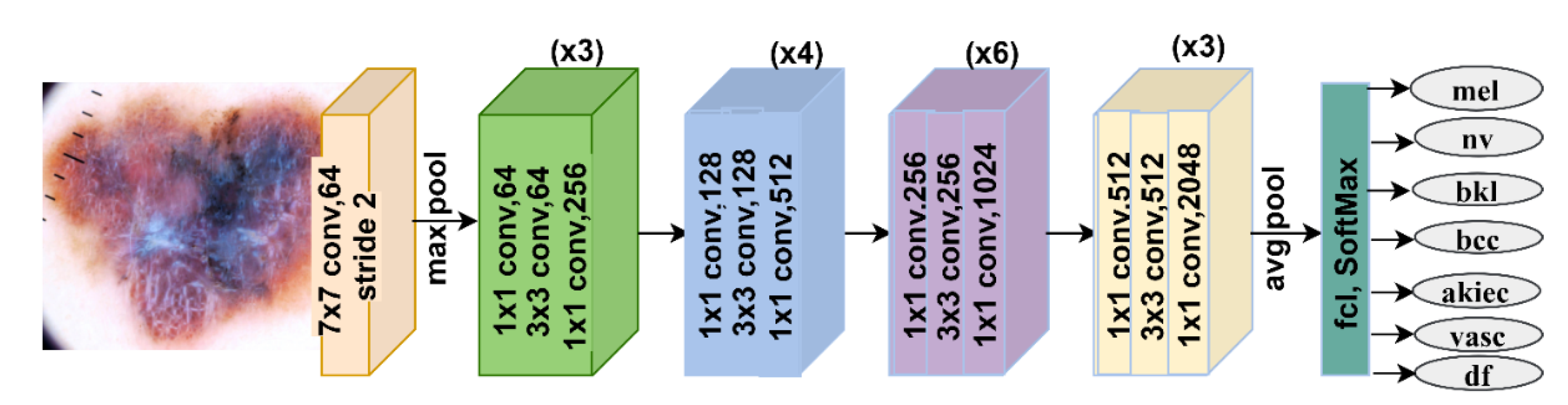
The ResNet-50 model contained 16 blocks with 177 layers divided into 49 convolutional layers, ReLU, batch normalization, one max-pooling layer, one average-pooling layer, one fully connected layer, and the softmax function. Seven and three classes were produced by the softmax function for the ISIC 2018 and PH2 datasets, respectively. ResNet-50 also contains 23.9 million parameters [44]. Figure 9 describes the basic architecture of ResNet-50 for diagnosing the ISIC 2018 dataset.

Table 1. The detailed structure of the convolutional neural network of the ResNet-50 model.

Layer Name	Tensor Size	Filter Size	Channel Number
	Input
Input Image	224 × 224 × 3	0	224
Conv-1	224 × 224 × 3	7 × 7	64
MaxPool	77 × 77 × 64	3 × 3	_
	38 × 38 × 64	1 × 1	64
Conv-2	38 × 38 × 64	3 × 3	64
	38 × 38 × 256	1 × 1	256
	19 × 19 × 128	1 × 1	128
Conv-3	19 × 19 × 128	3 × 3	128
	19 × 19 × 512	1 × 1	512
	10 × 10 × 256	1 × 1	256
Conv-4	10 × 10 × 256	3 × 3	256
	10 × 10 × 1024	1 × 1	1024
	5 × 5 × 512	1 × 1	512
Conv-5	5 × 5 × 512	3 × 3	512
	5 × 5 × 2048	1 × 1	2048
Avg pool	5 × 5 × 2048	7 × 7	_
Flath	5 × 5 × 2048	_	1
SoftMax	output units		7 or 3

describes the number of layers, the size of each filter, and the parameters of the ResNet-50 model.

AlexNet Model

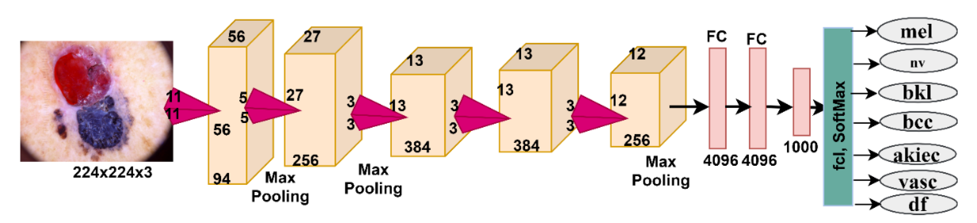
The AlexNet model contained 25 layers divided into five convolutional layers, three max-pooling layers, three fully connected layers, a classification-output layer, two leaking layers, and a softmax activation function. Seven and three classes were produced for the ISIC 2018 and PH2 datasets, respectively [45]. AlexNet contained 62 million parameters, 630 million connections, and 650,000 neurons. In Figure 10, the basic architecture of AlexNet for diagnosing the ISIC 2018 dataset is described. The number of layers, the size of each filter, and the parameters of the AlexNet model are described in

Table 2. Detailed structure of the AlexNet convolutional neural network.

Layer Name	Tensor Size		Filter Size	Parameters
	Input	Output
Input Image	227 × 227 × 3	227 × 227 × 3	0	0
Conv-1	227 × 227 × 3	55 × 55 × 96	11 × 11	34,944
MaxPool-1	55 × 55 × 96	27 × 27 × 96	3 × 3	0
Conv-2	27 × 27 × 96	27 × 27 × 256	5 × 5	614,656
MaxPool-2	27 × 27 × 256	13 × 13 × 256	3 × 3	0
Conv-3	13 × 13 × 256	13 × 13 × 384	3 × 3	885,120
Conv-4	13 × 13 × 384	13 × 13 × 384	3 × 3	1,327,488
Conv-5	13 × 13 × 384	13 × 13 × 256	3 × 3	884,992
MaxPool-3	13 × 13 × 256	6 × 6 × 256	3 × 3	0
FC-1	4096 × 1		1 × 1	37,752,832
FC-2	4096 × 1		1 × 1	16,781,312
FC-3	1000 × 1		1 × 1	4,097,000
Output	1000 × 1		0	0
SoftMax	output units			7 or 3
Total				62,378,344

.

CNNs have many layers to extract feature maps from the input images. The transfer learning technique was applied with the aim of transferring the experience gained from pre-training to perform new tasks on the ISIC 2018 and PH2 data sets. The knowledge gained when training convolutional neural networks were stored with this technology for more than a million images to obtain more than a thousand classes. Learning is transferred to solve new problems related to the classification of skin diseases. We aim to use CNNs for diagnosing skin diseases by comparing the results with traditional neural networks ANN and FFNN.

4. Experimental Results

4.1. Splitting Dataset and Environment Setup

The proposed systems were evaluated on the ISIC 2018 and PH2 datasets. The division of the two data sets is described in

Table 3. Splitting the two data set for training and testing.

Dataset	Total of Sample	80% for Training and Validation (80:20%)	20% for Testing	Total of Classes
ISIC 2018	1200	960	240	7 classes
PH2	200	160	40	3 classes

. First, the ISIC 2018 dataset, which contained 1200 images divided into seven diseases, was divided into 80% (960 images) for training and validation (80% and 20%; 678 and 192 images, respectively) and 20% (240 images) for testing. Then, the PH2 dataset, which contained 200 images, was divided into three diseases. The dataset was divided into 80% (160 images) for training and validation (80% and 20%; 128 and 32 images, respectively) and 20% (40 images) for evaluating the methods. All proposed systems were implemented with an Intel^® i5 processor, 8 GB RAM, 4 GB NVIDIA GeForce 940MX and Software by MATLAB 2018b.

4.2. Evaluation Metrics

For the performance of machine learning algorithms (ANN and FFNN) and deep learning (ResNet-50 and AlexNet) implemented on the ISIC 2018 and PH2 datasets, the following statistical measures were considered: accuracy, precision, sensitivity, specificity, and AUC. The following equations describe the evaluation of the proposed systems through a confusion matrix that contains all correctly classified cases (TP and TN) and incorrectly classified cases (FP and FN) [46]:

$$\mathrm{Accuracy}=\frac{\mathrm{TN}+\mathrm{TP}}{\mathrm{TN}+\mathrm{TP}+\mathrm{FN}+\mathrm{FP}}\times 100\%$$

(9)

$$\mathrm{Precision}=\frac{\mathrm{TP}}{\mathrm{TP}+\mathrm{FP}}\times 100\%$$

(10)

$$\mathrm{Sensitivity}=\frac{\mathrm{TP}}{\mathrm{TP}+\mathrm{FN}}\times 100\%$$

(11)

$$\mathrm{Specificity}=\frac{\mathrm{TN}}{\mathrm{TN}+\mathrm{FP}}\times 100$$

(12)

$$\mathrm{AUC}=\frac{\mathrm{True}\mathrm{Positive}\mathrm{Rate}}{\mathrm{False}\mathrm{Positive}\mathrm{Rate}}=\frac{\mathrm{Sensitivity}}{\mathrm{Specificity}}$$

(13)

where TP represented a sufferer case (skin disease) that was correctly classified, TN represented a sufferer case that was correctly classified as normal, FN represented a sufferer case (skin disease) classified as normal, and FP represented a normal case classified as skin disease.

4.3. Results of the ANN and FFNN Algorithms

Traditional neural networks are good tools for medical image diagnosis. The neural network process consists of the training and validation phases. Then, a testing phase of the quality of the performance of the system on new samples is conducted. In Figure 11, the training process for the ANN and FFNN algorithms is described. These algorithms consisted of an input layer with 220 neurons (number of features extracted from the previous stage), 10 hidden layers in which all the computations were performed, and an output layer containing seven classes for the ISIC 2018 dataset and three categories for the PH2 dataset.

4.3.1. Performance Analysis

The performance of the algorithms was analyzed by calculating the cross-entropy loss and the least-square error between the expected and actual output. In Figure 12, the errors during the training, validation, and testing phase are described. The performance of the ANN algorithm for the ISIC 2018 dataset is shown in Figure 12a. The best performance achieved at a value of 0.058987 occurred in epoch 48. In Figure 12b, the best performance of the ANN algorithm for the PH2 dataset is shown, achieving the best performance value of 0.020612, which occurred in epoch 22. The training stage was indicated by the color, the validation was indicated by the green color, the testing stage was indicated by the red color, and the best performance was indicated by the crossed line. The minimum error was obtained in the training data, with a more significant number of epochs. The training was stopped when validation was stopped, and the weights were set to specific values.

4.3.2. Gradient

In Figure 13, the gradient and validation values are described. In Figure 13a, the gradient value of the ANN algorithm is shown for the ISIC 2018 dataset. A value of 0.007904 was reached at epoch 54, and a validation value of six was reached at epoch 54. In Figure 13b, the gradient value of the ANN algorithm is described in the ISIC 2018 dataset. A value of 0.28647 was reached at epoch 28, and a validation value of six was reached at epoch 28.

4.3.3. Regression

Regression is a method for predicting continuous variable(s) based on other variable(s) values. The relationship between the actual and predicted outputs is accurate when R approaches 1.0. In Figure 14, the regression when evaluating the ISIC 2018 dataset using the FFNN algorithm is described. The relationship between the actual and predicted outputs was 92.35% during the training phase. The relationship was 75.85% during the validation phase and 78.18% during the testing phase. The total relationship was 87.30%.

4.3.4. Confusion Matrix

System performance outcomes were represented by a confusion matrix. The system performance metrics are extracted from them in such a matrix. All correctly classified samples, TP and TN, and incorrectly classified samples, FP and FN, were displayed in a confusion matrix. This section contains the confusion matrix for the ISIC 2018 and PH2 datasets for the ANN algorithm. The confusion matrix of the ISIC 2018 dataset is shown in Figure 15. The disease classes were represented as follows: MEL (class 1), VASC (class 2), DF (class 3), NV (class 4), AKIEC (class 5), BCC (class 6), and BKL (class 7). In Figure 16, which corresponds to the PH2 dataset, the disease classes were represented as follows: MEL (class 1), benign disease (class 2), and atypical disease (class 3).

In Figure 15 and

Table 4. The performance of the ANN and FFNN algorithms on the ISIC 2018 and PH2 datasets.

Classifier	Dataset	ISIC 2018	PH2
ANN	Accuracy %	95.3	97
	Precision %	94.63	95.97
	Sensitivity %	99.18	98.45
	Specificity %	94.87	96.07
	AUC %	96.93	97.23
FFNN	Accuracy %	95.24	97.91
	Precision %	91.69	97.09
	Sensitivity %	98.26	98.68
	Specificity %	92.21	97.14
	AUC %	95.03	97.89

, the results of the ANN algorithm for the ISIC 2018 dataset during the training, validation, testing, and overall results phase are described. An overall accuracy of 95.3% was achieved by the algorithm. During the training, validation, and testing phases, the accuracy rates reached by the ANN were 98.8%, 88.5%, and 88.5%, respectively.

In Figure 16, the results of the ANN algorithm for the PH2 dataset during the training, validation, testing, and overall results phase are described. An overall accuracy of 97% was reached by the algorithm. During the training, validation, and testing phases, accuracies of 98.5%, 93.9%, and 93.9% were reached by the method, respectively.

In Table 4, the performance of ANN and FFNN algorithms in detecting skin diseases on the ISIC 2018 and PH2 datasets was summarized. We noted that the ANN algorithm was superior to FFNN in diagnosing diseases in the ISIC 2018 dataset. First, to diagnose the ISIC 2018 dataset, the ANN algorithm reached an accuracy of 95.3%, precision of 94.63%, sensitivity of 99.18%, specificity of 94.87%, and AUC of 96.93%. At the same time, the FFNN algorithm reached an accuracy of 95.24%, precision of 91.69%, sensitivity of 98.26%, specificity of 92.21%, and AUC of 95.03%. Regarding the PH2 dataset, the FFNN algorithm outperformed the ANN algorithm. The FFNN algorithm reached an accuracy of 97.91%, precision of 97.09%, sensitivity of 98.68%, specificity of 97.14%, and AUC of 97.89%. At the same time, the ANN algorithm achieved accuracy of 97%, precision of 95.97%, sensitivity of 98.45%, specificity of 96.07%, and AUC of 97.23%.

4.3.5. Receiver Operating Characteristic (ROC)

The receiver operating characteristic (ROC) is a system performance curve for diagnosing a dataset during the training, validation, and testing phases. Colored lines represented curves for each class of diseases. Each color represented a disease assessment curve. The false-positive rate (FPR), known as specificity, was represented in the x-axis. The true positive rate (TPR), known as sensitivity, was represented in the y-axis. The ROC values of the ISIC 2018 dataset, consisting of seven disease classes described during the training, validation, and testing phases, are shown in Figure 17a. The ROC values of the PH2 dataset, composed of three disease classes, were described during the training, validation, and testing phases, as shown in Figure 17b. With an average value of seven classes, an accuracy rate of 96.93% was reached by ROC in the ISIC 2018 dataset. For the PH2 dataset with an average value of three classes, a rate of 97.23% was reached by ROC.

4.4. Results of the CNN Models

Here, the performance evaluation of ResNet-50 and AlexNet, two CNN networks, is shown during the image classification of the ISIC 2018 and PH2 datasets for the early detection of skin diseases. The two datasets were divided into 80% for training and validation (80% and 20%) and 20% for testing. The image size was standardized in the system to obtain robust results. In the ResNet-50 model, the images entered with a resolution of 224 × 224 × 3 pixels, whereas the resolution considered in the AlexNet model was 227 × 227 × 3 pixels. The output formats of the ResNet-50 and AlexNet models were determined by the softmax activation function. Seven and three disease classes were produced by the softmax function to identify and classify skin diseases in the ISIC 2018 and PH2 datasets, respectively. The performance of the ResNet-50 and AlexNet models depended on the parameters in each layer. For example, network performance depended on the filter size, stride, and padding of the convolutional layers. The extracted feature maps differed from layer to layer depending on the filters used. Classification accuracy is also affected by the size of the pooling layers. The CNN model tuning regarding the optimizer, learning rate, maximum epoch, mini-batch size, training time, and validation frequency are illustrated in

Table 5. Training parameter options for the ResNet-50 and AlexNet models.

Options	ResNet-50	AlexNet
training Options	adam	adam
Mini Batch Size	20	120
Max Epochs	6	12
Initial Learn Rate	0.0001	0.0001
Validation Frequency	5	50
Training time (min)	57 min 50 s	34 min 28 s
Execution Environment	GPU	GPU

. The proposed models were evaluated on the ISIC 2018 dataset, which contained 1200 images divided into seven classes, and the PH2 dataset, which contained 120 images divided into three classes.

The results of the ResNet-50 were better than those of AlexNet models, as shown in

Table 6. The performance of the ResNet-50 and AlexNet algorithms on the ISIC 2018 and PH2 datasets.

Classifier	Dataset	ISIC 2018	PH2
ResNet-50	Accuracy %	90	95.8
	Precision %	91.43	96.33
	Sensitivity %	89.37	95.64
	Specificity %	97.84	98.21
	AUC %	85	100
AlexNet	Accuracy %	85.3	91.7
	Precision %	85.42	92.66
	Sensitivity %	84.43	91.66
	Specificity %	97.71	96
	AUC %	96.81	100

. Thus, the ResNet-50 model has an essential role in the diagnostic accuracy of early detection of skin diseases. Superior performance in the early detection of skin diseases was achieved by the two models with images from the PH2 dataset than with images from the ISIC 2018 dataset. It was noted with the 2018 ISIC dataset, the ResNet-50 model reached an accuracy of 90%, precision of 91.43%, sensitivity of 89.37%, specificity of 97.84%, and AUC of 85%. With the PH2 dataset, an accuracy of 95.8%, precision of 96.33%, sensitivity of 95.64%, specificity of 98.21%, and AUC of 100% was reached by the ResNet-50 model. It was also noted that with the 2018 ISIC dataset, the AlexNet model reached an accuracy of 85.3%, the precision of 85.42%, the sensitivity of 84.43%, specificity of 97.71%, and AUC of 96.81%. With the PH2 dataset, an accuracy of 91.7%, precision of 92.66%, sensitivity of 91.66%, specificity of 96%, and AUC of 100% was reached.

The confusion matrices of the ResNet-50 model for early detection of skin diseases using the ISIC 2018 and PH2 datasets are shown in Figure 18. In the ISIC 2018 dataset, the diagnostic accuracy reached by the ResNet-50 model in each disease class was 100% for NV and MEL images, 87.5% for BKL images, 85% for BCC, AKIEC, and VASC images, and 80% for DF images. At the same time, the diagnostic accuracy reached by the ResNet-50 model was 100% for MEL images and 85.7% for images of benign and atypical diseases. The confusion matrices of the AlexNet model for the early detection of skin diseases in the ISIC 2018 and PH2 datasets are shown in Figure 19. For the PH2 dataset, the diagnostic accuracy at the level of each disease class reached by the AlexNet model was 100% for NV images, 98.3% for the MEL images, 83.3% for BKL images, 76.7% for BCC images, 73.3% for AKIEC images, 90% for VASC images, and 70% for DF images. For the PH2 dataset, the AlexNet model achieved a diagnostic accuracy of 100% for MEL images and 87.5% for benign and atypical disease images.

The ResNet-50 model performance regarding the ISIC 2018 and PH2 datasets considering the ROC from the AUC scale is shown in Figure 20. In that image, the closer the curve was to a right angle, the better the result, because it is close to 100%. AUC values of 85% and 100% were reached by the ResNet-50 model for the ISIC 2018 and PH2 datasets, respectively. The AlexNet model performance regarding the ISIC 2018 and PH2 datasets and considering the ROC from the AUC scale is shown in Figure 21. AUC values of 96.81% and 100% were obtained by the AlexNet model for the ISIC 2018 and PH2 datasets, respectively.

5. Discussion and Compare with Related Studies

5.1. Discussion of the Performance of the Proposed Systems

In this study, systems were developed using artificial intelligence techniques (e.g., machine learning and deep learning) to diagnose images of the ISIC 2018 and PH2 datasets for the early detection of skin diseases. The dataset was divided into 80% for training and validation phases (80% and 20%, respectively) and 20% for the testing phase. First, an automated learning system was developed based on segmentation methods, separating the lesion area from healthy skin and extracting the hybrid characteristics using three algorithms: LBP, GLCM, and DWT. A total of 220 features was produced using the three methods. These features were fed into the ANN and FFNN algorithms for diagnosing skin diseases. Two hundred and twenty features were entered, and these features were processed with 10 hidden layers. The two algorithms produced seven classes for the ISIC 2018 dataset and three classes for the PH2 dataset. It is worth noting that the highest accuracy of 95.24% for the ISIC 2018 dataset and 97.91% for the PH2 dataset was achieved using the FFNN algorithm. Accuracy rates of 95.3% for the ISIC 2018 dataset and 97% for the PH2 dataset were acquired using the ANN algorithm. Second, by using two deep learning models (e.g., ResNet-50 and AlexNet) to diagnose the ISIC 2018 and PH2 datasets for early detection of skin diseases. The ResNet-50 model performed better than the AlexNet model for both datasets. Accuracy rates of 90% for the ISIC 2018 dataset and 95.8% for the PH2 dataset were achieved using the ResNet-50 model. In contrast, an accuracy of 85.3% for the ISIC 2018 dataset and 91.7% for the PH2 dataset was obtained using the AlexNet model. We concluded that more accurate results were acquired by the ANN and FFNN algorithms than by CNN networks through the results mentioned above.

In the case of the ANN and FFNN algorithms, we used pretreatment and hair removal techniques, which helped us obtain more accurate results. However, accurate results for the early detection of skin diseases were obtained using the rest of the proposed systems.

The accuracy rates reached by each system in diagnosing each disease are described in

Table 7. The accuracy reached by each system in the diagnosis at the level of each disease.

Dataset	Diseases	Machine Learning		Deep Learning
		ANN	FFNN	ResNet-50	AlexNet
ISIC 2018	akiec	90	85	85	73.3
	bcc	99	100	85	76.7
	bkl	98.5	100	87.5	83.3
	df	92	17	80	70
	mel	97.5	92.5	100	96.3
	nv	95	98	100	100
	vasc	92	85	85	90
PH2	mel	95	98.8	100	100
	nv	95	87.5	85.7	87.5
	atypical	100	100	85.7	87.5

. In the ISIC 2018 dataset, the best accuracy for diagnosing AKIEC was reached by the ANN classifier, reaching 90%. The best accuracy for diagnosing BCC (100%) was obtained by the FFNN classifier. Then, the best accuracy for diagnosing BKL was reached by the FFNN classifier, with 100% accuracy. The ANN classifier had the best accuracy (92%) for diagnosing DF. The best accuracy for diagnosing MEL was reached using the ResNet-50 model (100%). The highest accuracy (100%) for diagnosing NV was reached by the ResNet-50 and AlexNet models. Finally, the best accuracy for the diagnosis of VASC cases was reached by the ANN classifier, with a 92% accuracy rate.

Regarding the PH2 dataset, the best accuracy for MEL disease diagnosis (100%) was reached by ResNet-50 and AlexNet. The best accuracy for NV disease diagnosis was reached by the ANN classifier (95% accuracy). Finally, the best accuracy rate (100%) for diagnosing atypical disease cases was achieved using the ANN and FFNN classifiers. The performance comparison of the proposed systems for diagnosing skin diseases at the level of each disease is shown in Figure 22.

5.2. Comparison with Related Studies

In this section, a comparison of the performance results of the proposed systems with previous related studies is presented in

Table 8. Comparison of the performance of the proposed systems with the existing systems.

Previous Studies	Accuracy %	Precision %	Sensitivity %	Specificity %	AUC %
Sameena, et al. [47]	80		79	81	-
Bhumika, et al. [48]	66	69.08	66	-	-
Serban, et al. [49]	80.52	-	72	89	-
Roberta, et al. [50]	75.8	-	69.4	82.2	-
Parvathaneni, et al. [51]	85.34		88.24	92	-
Gong, et al. [52]	89.3	-	37.6	95.4	85.6
Reisinho, et al. [53]	78.93	-	78.98	92.99	-
Proposed model by ANN	95.3	94.63	99.18	94.87	96.93
Proposed model by ResNet-50	90	91.43	89.37	97.84	85

. The results of the proposed methods show that they have a better diagnostic performance than the previous related works. The performance was compared through accuracy, precision, sensitivity, specificity, and AUC; the table shows that the proposed systems have all the standards, while the other systems lack some of the measures. All previous systems achieved an accuracy between 89.3% and 60%, while the proposed system ANN achieved 95.3% and ResNet-50 achieved 90%. Regarding sensitivity, the previous systems achieved a rate ranging between 37.6% and 88.24%, while the proposed system ANN achieved a rate of 99.18% and ResNet-50 achieved 89.37%. As for specificity, the previous systems achieved a percentage ranging between 81% and 95.4%, while the proposed method ResNet-50 achieved 97.84%. Figure 23 display the performance of the proposed systems with the performance of some related previous studies.

6. Conclusions

Skin diseases are spreading nowadays in many countries due to long-term exposure to the sun and weather changes. Many skin diseases must be diagnosed and treated early to avoid severe consequences for the health of affected individuals. Melanoma (skin cancer) is considered one of the most dangerous types of skin disease, and it must be diagnosed before it penetrates the internal tissues of the skin and spreads from one place to another in the body. In this work, we developed diagnostic systems based on artificial intelligence to diagnose the images of two standard datasets, ISIC 2018 and PH2, for the early detection of skin diseases. The images in the two data sets were divided into 80% for training and validation (80% and 20%, respectively) and 20% for testing. In the first step of the proposed early detection using these proposed systems, ANN and FFNN algorithms were implemented to diagnose the features extracted by hybrid methods (e.g., LBP, GLCM, and DWT). The features of the three methods were combined and collected in a features matrix so that each vector (image) contained 220 essential features representing the disease types. In the second step, CNNs models were implemented, ResNet-50 and AlexNet, based on transfer learning. The results obtained with traditional neural networks (ANN and FFNN) were compared with CNN networks (ResNet-50 and AlexNet). It was noted that ANN and FFNN algorithms performed better than two CNN models, ResNet-50 and AlexNet. Despite applying many optimization techniques and extracting the features by hybrid methods between three algorithms, there are some limitations and challenges encountered in the study, which are represented in the significant similarity between the features of some diseases, which causes confusion for the classification algorithms when making a diagnosis. Solving these limitations in the future will require extracting features from various algorithms using traditional methods and combining them with deep feature maps extracted by CNN models, as well as applying hybrid methods between machine learning algorithms and deep learning models by using two blocks. In the first block, the deep features are extracted by CNN models. The second block is one of the machine learning algorithms that is fed with the output of the first block for classifying dermatology.

References

1. Rosenbaum, S. Health Cares. Nation 2008, 22. Available online: https://hsrc.himmelfarb.gwu.edu/sphhs_policy_informal/22 (accessed on 18 November 2021).
2. Proksch, E.; Brandner, J.M.; Jensen, J.M. The skin: An indispensable barrier. Exp. Dermatol. 2008, 17, 1063–1072. [Google Scholar] [CrossRef] [PubMed]
3. Sakuma, T.H.; Maibach, H.I. Oily skin: An overview. Ski. Pharmacol. Physiol. 2012, 25, 227–235. [Google Scholar] [CrossRef] [PubMed]
4. Nasir, M.; Khan, M.A.; Sharif, M.; Javed, M.Y.; Saba, T.; Ali, H.; Tariq, J. Melanoma Detection and Classification using Computerized Analysis of Dermoscopic Systems: A Review. Curr. Med. Imaging Former. Curr. Med. Imaging Rev. 2019, 16, 794–822. [Google Scholar] [CrossRef] [PubMed]
5. Saba, T.; Khan, M.A.; Rehman, A.; Marie-Sainte, S.L. Region Extraction and Classification of Skin Cancer: A Heterogeneous framework of Deep CNN Features Fusion and Reduction. J. Med. Syst. 2019, 43, 289. [Google Scholar] [CrossRef]
6. Nasir, M.; Khan, M.A.; Sharif, M.; Lali, I.U.; Saba, T.; Iqbal, T. An improved strategy for skin lesion detection and classification using uniform segmentation and feature selection based approach. Microsc. Res. Tech. 2018, 81, 528–543. [Google Scholar] [CrossRef]
7. Zhang, B.; Zhou, X.; Luo, Y.; Zhang, H.; Yang, H.; Ma, J.; Ma, L. Opportunities and Challenges: Classification of Skin Disease Based on Deep Learning. Chin. J. Mech. Eng. 2021, 34, 112. [Google Scholar] [CrossRef]
8. Herman, C. Emerging technologies for the detection of melanoma: Achieving better outcomes. Clin. Cosmet. Investig. Dermatol. 2012, 5, 195. [Google Scholar] [CrossRef] [Green Version]
9. LeCun, Y.; Bengio, Y.; Hinton, G. Deep learning. Nature 2015, 521, 436–444. [Google Scholar] [CrossRef]
10. Khan, M.A.; Muhammad, K.; Sharif, M.; Albuquerque, V.H.C. Multi-Class Skin Lesion Detection and Classification via Teledermatology. IEEE J. Biomed. Health Inform. 2021, 25, 4267–4275. [Google Scholar] [CrossRef]
11. Khan, M.A.; Zhang, Y.D.; Sharif, M.; Akram, T. Pixels to Classes: Intelligent Learning Framework for Multiclass Skin Lesion Localization and Classification. Comput. Electr. Eng. 2021, 90, 106956. [Google Scholar] [CrossRef]
12. Qin, Z.; Liu, Z.; Zhu, P.; Xue, Y. A GAN-based image synthesis method for skin lesion classification. Comput. Methods Programs Biomed. 2020, 195, 105568. [Google Scholar] [CrossRef] [PubMed]
13. Tschandl, P.; Sinz, C.; Kittler, H. Domain-specific classification-pretrained fully convolutional network encoders for skin lesion segmentation. Comput. Biol. Med. 2019, 104, 111–116. [Google Scholar] [CrossRef]
14. Sreelatha, T.; Subramanyam, M.V.; Prasad, M.G. Early detection of skin cancer using melanoma segmentation technique. J. Med Syst. 2019, 43, 190. [Google Scholar] [CrossRef]
15. Chatterjee, S.; Dey, D.; Munshi, S. Integration of morphological preprocessing and fractal based feature extraction with recursive feature elimination for skin lesion types classification. Comput. Methods Programs Biomed. 2019, 178, 201–218. [Google Scholar] [CrossRef]
16. Al-Masni, M.A.; Kim, D.H.; Kim, T.S. Multiple skin lesions diagnostics via integrated deep convolutional networks for segmentation and classification. Comput. Methods Programs Biomed. 2020, 190, 105351. [Google Scholar] [CrossRef] [PubMed]
17. Alzubaidi, L.; Al-Amidie, M.; Al-Asadi, A.; Humaidi, A.J.; Al-Shamma, O.; Fadhel, M.A.; Zhang, J.; Santamaría, J.; Duan, Y. Novel Transfer Learning Approach for Medical Imaging with Limited Labeled Data. Cancers 2021, 13, 1590. [Google Scholar] [CrossRef] [PubMed]
18. Liu, Y.P.; Wang, Z.; Li, Z.; Li, J.; Li, T.; Chen, P.; Liang, R. Multiscale ensemble of convolutional neural networks for skin lesion classification. IET Image Process. 2021, 15, 2309–2318. [Google Scholar] [CrossRef]
19. Ding, S.; Zheng, J.; Liu, Z.; Zheng, Y.; Chen, Y.; Xu, X.; Lu, J.; Xie, J. High-resolution dermoscopy image synthesis with conditional generative adversarial networks. Biomed. Signal Process. Control 2021, 64, 102224. [Google Scholar] [CrossRef]
20. Surówka, G.; Ogorzalek, M. Wavelet-based logistic discriminator of dermoscopy images. Expert Syst. Appl. 2021, 167, 113760. [Google Scholar] [CrossRef]
21. Iqbal, I.; Younus, M.; Walayat, K.; Kakar, M.U.; Ma, J. Automated multi-class classification of skin lesions through deep convolutional neural network with dermoscopic images. Comput. Med. Imaging Graph. 2021, 88, 101843. [Google Scholar] [CrossRef]
22. Sikkandar, M.Y.; Alrasheadi, B.A.; Prakash, N.B.; Hemalakshmi, G.R.; Mohanarathinam, A.; Shankar, K. Deep learning based an automated skin lesion segmentation and intelligent classification model. J. Ambient Intell. Humaniz. Comput. 2021, 12, 3245–3255. [Google Scholar] [CrossRef]
23. Ali, M.S.; Miah, M.S.; Haque, J.; Rahman, M.M.; Islam, M.K. An enhanced technique of skin cancer classify cation using deep convolutional neural network with transfer learning models. Mach. Learn. Appl. 2021, 5, 100036. [Google Scholar] [CrossRef]
24. Kim, D.; Hong, B.W. Unsupervised Feature Elimination via Generative Adversarial Networks: Application to Hair Removal in Melanoma Classification. IEEE Access 2021, 9, 42610–42620. [Google Scholar] [CrossRef]
25. Tyagi, A.; Mehra, R. An optimized CNN based intelligent prognostics model for disease prediction and classification from Dermoscopy images. Multimed. Tools Appl. 2020, 79, 26817–26835. [Google Scholar] [CrossRef]
26. Ahmad, B.; Jun, S.; Palade, V.; You, Q.; Mao, L.; Zhongjie, M. Improving Skin Cancer Classification Using Heavy-Tailed Student T-Distribution in Generative Adversarial Networks (TED-GAN). Diagnostics 2021, 11, 2147. [Google Scholar] [CrossRef]
27. Molina-Molina, E.O.; Solorza-Calderón, S.; Álvarez-Borrego, J. Classification of dermoscopy skin lesion color-images using fractal-deep learning features. Appl. Sci. 2020, 10, 5954. [Google Scholar] [CrossRef]
28. Adegun, A.A.; Viriri, S. FCN-based DenseNet framework for automated detection and classification of skin lesions in dermoscopy images. IEEE Access 2020, 8, 150377–150396. [Google Scholar] [CrossRef]
29. Khan, M.A.; Akram, T.; Sharif, M.; Kadry, S.; Nam, Y. Computer Decision Support System for Skin Cancer Localization and Classification. Comput. Mater. Contin. 2021, 68, 1041–1064. [Google Scholar] [CrossRef]
30. Khan, M.A.; Muhammad, K.; Sharif, M.; Akram, T.; Kadry, S. Intelligent fusion-assisted skin lesion localization and classification for smart healthcare. Neural Comput. Appl. 2021, 20, 1–16. [Google Scholar] [CrossRef]
31. Khan, M.A.; Sharif, M.; Akram, T.; Kadry, S.; Hsu, C.H. A two-stream deep neural network-based intelligent system for complex skin cancer types classification. Int. J. Intell. Syst. 2021. [Google Scholar] [CrossRef]
32. Khan, M.A.; Sharif, M.; Akram, T.; Damaševičius, R.; Maskeliūnas, R. Skin Lesion Segmentation and Multiclass Classification Using Deep Learning Features and Improved Moth Flame Optimization. Diagnostics 2021, 11, 811. [Google Scholar] [CrossRef] [PubMed]
33. Tschandl, P.; Rinner, C.; Apalla, Z.; Argenziano, G.; Codella, N.; Halpern, A.; Kittler, H. Human–computer collaboration for skin cancer recognition. Nat. Med. 2020, 26, 1229–1234. [Google Scholar] [CrossRef]
34. ADDI. Automatic Computer-Based Diagnosis System for Dermoscopy Images. Available online: https://www.fc.up.pt/addi/ph2%20database.html (accessed on 10 December 2021).
35. Kiani, K.; Sharafat, A.R. E-shaver: An improved DullRazor® for digitally removing dark and light-colored hairs in dermoscopic images. Comput. Biol. Med. 2011, 41, 139–145. [Google Scholar] [CrossRef]
36. Senan, E.M.; Jadhav, M.E.; Kadam, A. Classification of PH2 Images for Early Detection of Skin Diseases. In Proceedings of the 2021 6th International Conference for Convergence in Technology (I2CT), Maharashtra, India, 2–4 April 2021; pp. 1–7. [Google Scholar] [CrossRef]
37. Senan, E.M.; Jadhav, M.E. Techniques for the Detection of Skin Lesions in PH 2 Dermoscopy Images Using Local Binary Pattern (LBP). In Proceedings of the International Conference on Recent Trends in Image Processing and Pattern Recognition, Aurangabad, India, 3–4 January 2020; pp. 14–25. [Google Scholar] [CrossRef]
38. Livieris, I.E. Improving the Classification Efficiency of an ANN Utilizing a New Training Methodology. Informatics 2019, 6, 1. [Google Scholar] [CrossRef] [Green Version]
39. Huang, M.L.; Chou, Y.C. Combining a gravitational search algorithm, particle swarm optimization, and fuzzy rules to improve the classification performance of a feed-forward neural network. Comput. Methods Programs Biomed. 2019, 180, 105016. [Google Scholar] [CrossRef]
40. Jahnavi, M. Introduction to Neural Networks. Advant. Appl. 2021. Available online: https://towardsdatascience.com/introduction-to-neural-networks-advantages-and-applications-96851bd1a207 (accessed on 1 December 2021).
41. Alsaade, F.W.; Aldhyani, T.H.; Al-Adhaileh, M.H. Developing a Recognition System for Diagnosing Melanoma Skin Lesions Using Artificial Intelligence Algorithms. Comput. Math. Methods Med. 2021, 2021, 9998379. [Google Scholar] [CrossRef]
42. Acharya, U.R.; Oh, S.L.; Hagiwara, Y.; Tan, J.H.; Adam, M.; Gertych, A.; San Tan, R. A deep convolutional neural network model to classify heartbeats. Comput. Biol. Med. 2017, 89, 389–396. [Google Scholar] [CrossRef]
43. Agarap, A.F. Deep Learning Using Rectified Linear Units (ReLU). Available online: https://arxiv.org/abs/1803.08375v2 (accessed on 1 December 2021).
44. Mohammed, B.A.; Senan, E.M.; Rassem, T.H.; Makbol, N.M.; Alanazi, A.A.; Al-Mekhlafi, Z.G.; Almurayziq, T.S.; Ghaleb, F.A. Multi-Method Analysis of Medical Records and MRI Images for Early Diagnosis of Dementia and Alzheimer’s Disease Based on Deep Learning and Hybrid Methods. Electronics 2021, 10, 2860. [Google Scholar] [CrossRef]
45. Senan, E.M.; Fawaz, W.A.; Mohammed, I.A.; Theyazn, H.H.; Mosleh, H.A. Classification of histopathological images for early detection of breast cancer using deep learning. J. Appl. Sci. Eng. 2021, 24, 323–329. [Google Scholar] [CrossRef]
46. Senan, E.M.; Al-Adhaileh, M.H.; Alsaade, F.W.; Aldhyani, T.H.; Alqarni, A.A.; Alsharif, N.; Uddin, M.I.; Alahmadi, A.H.; E Jadhav, M.; Alzahrani, M.Y. Diagnosis of Chronic Kidney Disease Using Effective Classification Algorithms and Recursive Feature Elimination Techniques. J. Healthc. Eng. 2021, 2021, 1004767. [Google Scholar] [CrossRef] [PubMed]
47. Pathan, S.; Prabhu, K.G.; Siddalingaswamy, P.C. Automated detection of melanocytes related pigmented skin lesions: A clinical framework. Biomed. Signal Process. Control 2019, 51, 59–72. [Google Scholar] [CrossRef]
48. Parmar, B.; Talati, B. Automated Melanoma Types and Stages Classification for dermoscopy images. In Proceedings of the 2019 Innovations in Power and Advanced Computing Technologies (i-PACT), Vellore, India, 22–23 March 2019; Volume 2019. [Google Scholar] [CrossRef]
49. Jianu, S.R.S.; Ichim, L.; Popescu, D. Automatic Diagnosis of Skin Cancer Using Neural Networks. In Proceedings of the 2019 11th International Symposium on Advanced Topics in Electrical Engineering, Bucharest, Romania, 28–30 March 2019; pp. 1–4. [Google Scholar] [CrossRef]
50. Oliveira, R.B.; Pereira, A.S.; Tavares, J.M.R. Computational diagnosis of skin lesions from dermoscopic images using combined features. Neural Comput. Appl. 2018, 31, 6091–6111. [Google Scholar] [CrossRef] [Green Version]
51. Srinivasu, P.N.; SivaSai, J.G.; Ijaz, M.F.; Bhoi, A.K.; Kim, W.; Kang, J.J. Classification of Skin Disease Using Deep Learning Neural Networks with MobileNet V2 and LSTM. Sensors 2021, 21, 2852. [Google Scholar] [CrossRef]
52. Gong, A.; Yao, X.; Lin, W. Classification for Dermoscopy Images Using Convolutional Neural Networks Based on the Ensemble of Individual Advantage and Group Decision. IEEE Access 2020, 8, 155337–155351. [Google Scholar] [CrossRef]
53. Reisinho, J.; Coimbra, M.; Renna, F. Deep Convolutional Neural Network Ensembles for Multi-Classification of Skin Lesions from Dermoscopic and Clinical Images. In Proceedings of the Annual International Conference of the IEEE Engineering in Medicine and Biology Society, Montreal, QC, Canada, 20–24 July 2020; Volume 2020, pp. 1940–1943. [Google Scholar] [CrossRef]
Figure 1. Methodology for classifying the ISIC 2018 and PH2 datasets used in this study.
Electronics 10 03158 g001
Figure 2. Samples of skin diseases obtained from the ISIC 2018 dataset.
Electronics 10 03158 g002
Figure 3. Samples of skin diseases obtained from the PH2 dataset.
Electronics 10 03158 g003
Figure 4. The image of a skin lesion before (left) and after (right) the hair removal process using the Dullrazor technique.
Electronics 10 03158 g004
Figure 5. Enhancement and segmentation process for some images from the ISIC 2018 dataset.
Electronics 10 03158 g005
Figure 6. Enhancement and segmentation process for some images from the PH2 dataset.
Electronics 10 03158 g006
Figure 7. The hybrid LBP, GLCM, and DWT algorithms used to extract features from the analyzed images.
Electronics 10 03158 g007
Figure 8. The architectures of the ANN and FFNN algorithms. (a) The architecture of ANN and FFNN from the ISIC 2018 dataset. (b) The architecture of ANN and FFNN from the PH2 dataset.
Electronics 10 03158 g008
Figure 9. The structure of the ResNet-50 model used in this study.
Electronics 10 03158 g009
Figure 10. The structure of the AlexNet model used in this study.
Electronics 10 03158 g010
Figure 11. The training of the process of the ANN algorithm, considering the different datasets used. (a) The ISIC 2018 dataset. (b) The PH2 dataset.
Electronics 10 03158 g011
Figure 12. Performance plot of the training of the ANN algorithm considering the datasets used. (a) The ISIC 2018 dataset. (b) The PH2 dataset.
Electronics 10 03158 g012
Figure 13. The training gradient displays of the ANN algorithm considering the datasets used. (a) The ISIC 2018 dataset. (b) The PH2 dataset.
Electronics 10 03158 g013
Figure 14. The displays of the regression values of the FFNN training algorithm for the ISIC 2018 dataset.
Electronics 10 03158 g014
Figure 15. Confusion matrix for the ANN algorithm of the ISIC 2018 dataset.
Electronics 10 03158 g015
Figure 16. Confusion matrix for the ANN algorithm of the PH2 dataset.
Electronics 10 03158 g016
Figure 17. Displays the ROC of the ANN algorithm: (a) ISIC 2018 data set and (b) PH2 data set.
Electronics 10 03158 g017
Figure 18. Confusion matrices for the ResNet-50 model considering the different datasets used. (a) The ISIC 2018 dataset. (b) The PH2 dataset.
Electronics 10 03158 g018
Figure 19. Confusion matrices for the AlexNet model considering the different datasets used. (a) The ISIC 2018 dataset. (b) The PH2 dataset.
Electronics 10 03158 g019
Figure 20. The ROC values reached by the ResNet-50 model considering the different datasets used. (a) The ISIC 2018 dataset. (b) The PH2 dataset.
Electronics 10 03158 g020
Figure 21. The ROC values reached by the AlexNet model considering the different datasets used. (a) The ISIC 2018 dataset. (b) The PH2 dataset.
Electronics 10 03158 g021
Figure 22. Performance comparison of the proposed systems for the early diagnosis of each skin disease analyzed in this study.
Electronics 10 03158 g022
Figure 23. Comparing the performance of the proposed systems with some relevant previous studies.
Electronics 10 03158 g023