An Improved Initialization Method for Monocular Visual-Inertial SLAM

Abstract

In the aim of improving the positioning accuracy of the monocular visual-inertial simultaneous localization and mapping (VI-SLAM) system, an improved initialization method with faster convergence is proposed. This approach is classified into three parts: Firstly, in the initial stage, the pure vision measurement model of ORB-SLAM is employed to make all the variables visible. Secondly, the frequency of the IMU and camera was aligned by IMU pre-integration technology. Thirdly, an improved iterative method is put forward for estimating the initial parameters of IMU faster. The estimation of IMU initial parameters is divided into several simpler sub-problems, containing direction refinement gravity estimation, gyroscope deviation estimation, accelerometer bias, and scale estimation. The experimental results on the self-built robot platform show that our method can up-regulate the initialization convergence speed, simultaneously improve the positioning accuracy of the entire VI-SLAM system.

1. Introduction

Visual simultaneous localization and mapping (VSLAM) techniques allow mobile robots [1,2] and VR/AR devices [3,4] to be aware of their surrounding scene, while carrying on the self-localization in the unknown environments. In recent years, many visual SLAM methods have been studied, such as multi-sensor fusion SLAM (e.g., visual-inertial, visual-LIDAR, and/or visual-GPS), deep learning SLAM, multi-agent SLAM, as well this technology has attracted a lot of interest in the emerging contexts of 5G/6G communications, since directional antenna arrays and higher bandwidths can be fruitfully exploited to achieve high accuracy and 5G/6G SLAM [5,6,7]. The SLAM system based on pure visual sensors has certain problems in robustness and accuracy, which limits its application in the field of terrestrial mobile robots. The monocular camera is not accurate in comparison with a binocular camera, but the computing complexity is lower, the IMU sensor can solve the problem of tracking failure and low precision when the monocular camera moves into the challenging environment (less texture and/or lighting changes) by using the IMU pre-integration technology and EKF/nonlinear optimization methods. On the other hand, the visual sensor can make up for the cumulative drift of the IMU [8]. Indeed, such information is crucial when operating in harsh propagation environments (e.g., rich of multipath) where the typical GNSS information is highly inaccurate or completely unavailable [9]. Now, the monocular visual-inertial SLAM system has become a hot topic which contains strap down inertial measurement units (IMU) and monocular vision sensors to provide a low-cost, lightweight, and high-quality solution for most positioning and navigation applications in an indoor and outdoor environment. For simultaneous interpreting of multiple sensor measurements from various sensor frames, a process of initial parameters estimation and calibration is essential. The camera only needs to be calibrated once because it does not change over time, and the IMU sensor must be initialized before each use. This paper focuses on the IMU’s initial values estimation. The IMU initialization process is designed to evaluate as fast as possible for the initial parameters with the initial IMU biases (gyroscope and accelerometer biases), gravity, and scale for the process of later numerical optimization. Once the parameters are triumphantly acquired, inertial measurement can be employed to enhance the robustness and accuracy of the continuous tracking and then find the measurement scale of a three-dimensional visual map, which cannot be obtained with a pure monocular SLAM system. Currently, the tightly-coupled nonlinear optimization approach for visual-inertial SLAM is widely applied, almost the state-of-the-art frameworks, for instance, OKVIS [10], VI-ORBSLAM [11], VI-DSO [12], and VINS-MONO [13] cannot have a good performance without an efficient initialization process. Especially, the convergence speed of initial estimation has a significant effect on the whole system.

Generally, the initialization of the monocular VI-SLAM system is a fragile but significant step. The former visual inertia initialization methods can be divided into joint methods together with disjoint methods [14]. The pros and cons of the initialization methods are shown in

Table 1. Pros and cons of the initialization methods.

Classification	Pros	Cons	Typical Studies
Joint method	With small-scale errors. Fast convergence speed.	lead to bad solutions under conditions of the spurious tracks. The estimation accuracy is not high enough.	Martinelli, A. [15,16] Campos, C. [17]
Disjoint method	The initialization estimation accuracy is high.	Initial estimation is slow and unstable. Rely on the monocular visual SLAM process.	Murata, R. [11]

.

The joint visual-inertial initialization approach is introduced through Martinelli at first, which is named closed-form solution. However, this research [15] expressed only in theory and then demonstrated by the simulation of general Gaussian motions, the application of MAV is not feasible. So this method is later modified in [16], not only increasing the estimation of gyroscope bias but also is a successful implementation of actual data from quadrotor MAV. The latest work of [17] put forward a robust and fast initialization approach according to [15,16]. The accuracy is improved through several visual-inertial bundle adjustments (BA), and the robustness of the system is enhanced with the addition of consensus and observability tests. As it is tested on the dataset of Euros [18], it is proved to be consistently initialized with scale errors is less than five percent. However, those initialization methods have several limitations:

• An ideal hypothesis in which all features are tracked in perspective should be contented. However, it can lead to bad solutions under conditions of spurious tracks.
• Compared with [19], the disjoint visual-inertial initialization method, the accuracy of the joint method is lower. To improve it, a lot of frames and tracks are usually added, which leads to the computational cost being so high that the real-time performance is unfeasible.
• The method in [17] works only at 20% of trajectory points. If the system requires to be started immediately, this may be a problem in robot use.

The disjoint visual-inertial initialization approach, i.e., loosely couple method, depends on a very accurate visual measurement model in the initial stage. This method is first applied by Mur-Artal and later adapted in [11,20] with a good performance on the public dataset. In particular, the motion of MAV with metric scale can be recovered with a small error, and the accuracy of positioning is maintained at centimeter-level [11]. However, this approach also exists several limitations:

• The process of initial estimation is slow and unstable. On account of the inertial parameters being evaluated through solving a set of the linear equations in various steps utilizing the least square method, it requires an excellent iterative strategy that makes fast convergence. However, the convergence speed in [11] is not reliable enough for all variables estimation. it can be a problem for many real applications.
• Initialization is fragile. As the method requires running monocular visual SLAM in advance for finding the accurate inertial parameters. If the visual part gets lost, the inertial system will not be launched immediately.

In summary, there are several initialization methods have been studied for the monocular VI-SLAM system. However, few researchers have tried to improve it from the perspective of non-linear optimization. In the current work, an improved initialization approach that is by the disjoint method is proposed. First, in the initial stage, the pure vision measurement model of ORB-SLAM2 is employed to make all the variables visible. Second, the frequency of the IMU camera was aligned by IMU pre-integration technology [21]. Third, the IMU initialization process, which is highlighted in a dotted block diagram with red color. It is divided into several simpler sub-problems, containing direction refinement gravity estimation, gyroscope deviation estimation, scale estimation as well as accelerometer deviation. In this work, an improved iterative method is put forward for estimating the initial parameters of IMU faster. The experimental outcomes on a real mobile robot demonstrate excellent performance while our initialization method is integrated into the VI-SLAM system which is based on the ORB-SLAM2 skeleton [19,22].

The rest of the current paper is organized as below: We introduce the preparatory work in Section 2. Then the core part of this paper, the IMU initialization process, is illustrated in Section 3. Section 4 introduces the real-time experiment for the mobile robot. Section 5 gives the summaries and the future work.

2. Preliminaries

In the present section, the necessary notation and the monocular visual-inertial coordinate frames and visual measurement model are briefly reviewed, then the IMU pre-integration on the manifold is described in the following sections.

2.1. Notation

In this paper, we aim to estimate gyroscope bias, gravity, accelerometer bias together with visual scale in the visual-inertial initialization stage. $SO(3)$ represents a special orthogonal group: Lie group, and $so(3)$ is the corresponding Lie algebra. The vectors are uniformly expressed in italics, the reference frame is marked with a right subscript, e.g., $A_V$ for the vector $A$ expressed in frame {$\mathrm{V}$}. If a vector describes the relative transformation from one reference frame to another frame, e.g., $A_{CB}$ for the vector that defines the translation from camera frame {C} to IMU body frame {B}. The correlations between camera frame {C} and IMU body frame {B} is defined by scale factor $s$ is considered:

$$\begin{array}{l}{R}_{WB}=R_{WC}·R_{CB}\\ P_{WB}=R_{WC}·P_{CB}+s·P_{WC}\end{array}$$

(1)

in which $s$ represents visual scale, $P_{(.)}$ and $R_{(.)}$ represent the translation and rotation vector between two coordinate frames, respectively. The subscript ${(.)}_{WB}$ indicates the world frame {W} to IMU body frame {B}, The subscript ${(.)}_{WC}$ indicates the world frame {W} to camera frame {C}, The subscript ${(.)}_{CB}$ indicates the camera frame {C} to IMU body frame {B}.

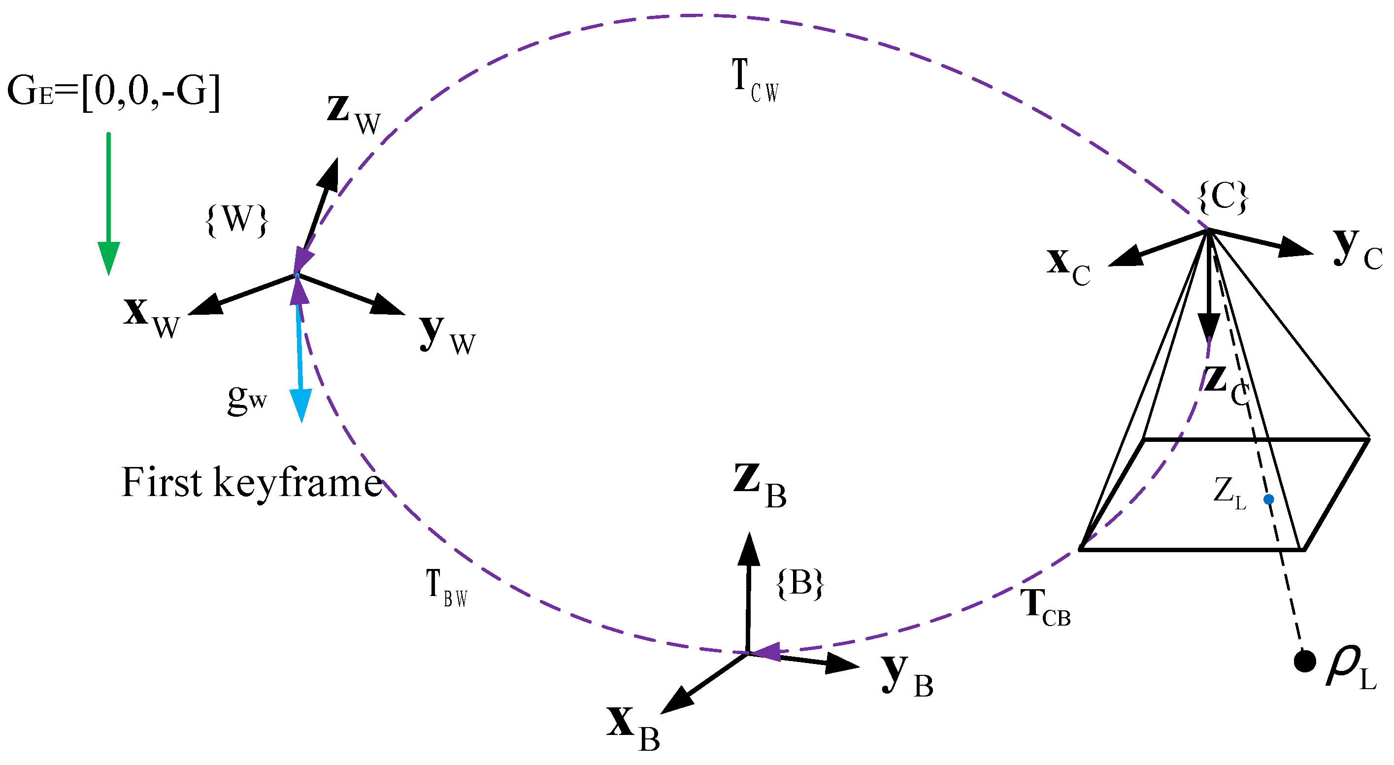
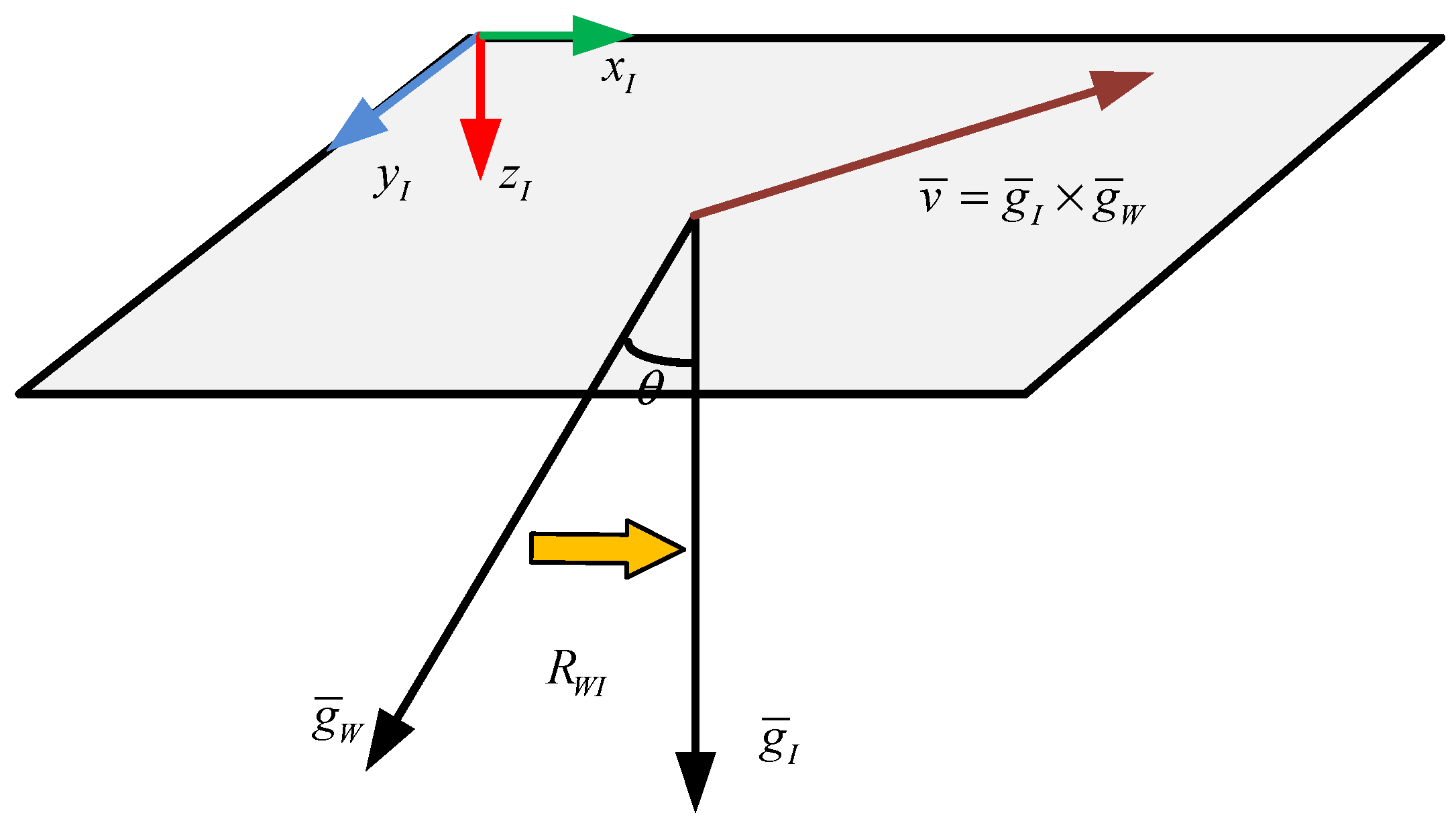
2.2. Coordinate Frames

The transformation between the coordinate frames is shown in Figure 1. Since the measurements of inertial and visual odometry are changed over time. However, the absolute pose is needed in the pre-fixed reference frame. Therefore, it is assumed that the reference frame of our system coincides with the first keyframe which is determined by the pure visual SLAM. In this work, the $G_E$ represents the gravity in the inertial frame {E} of earth. The $g_w$ represents the gravity in the world coordinate system {W}. The first keyframe is assumed as a reference frame. The external parameter matrix $T_{CB}$ is described as follows 4 × 4 matrix:

$$T_{CB}={\left[\begin{array}{cc}{R}_{CB}& T_{CB}\\ \stackrel{\rightharpoonup }{0}& 1\end{array}\right]}_{4\times 4}$$

(2)

where $R_{CB}$ and $T_{CB}$ represent the rotation and translation matrix/vector between camera frame {C} and body frame {B} is calibrated in advance.

2.3. Visual Measurement Model

The ORB-SLAM2 [19,22] visual measurement model is adopted for the initial pose estimation. The system consists of the following three parallel threads, i.e., tracing, local mapping along with loop closing. While the tracking together with local mapping threads is applied in the initialization stage. The tracking part is responsible for deciding whether to treat the new frame as a key. After inserting the new key, the associated IMU pre-integration model is calculated between two consecutive keyframes. In this work, we adopt the conventional visual model with the visual projection function $\pi (.)$, which converts 3-dimensional points $\{x_c,y_c,z_c\}$ in the camera frame into a 2-dimensional image coordinate $\{u,v\}$.

$$\pi (X_C)=\left[\begin{array}{l}{f}_u\frac{x_c}{z_c}+c_u\\ f_v\frac{y_c}{z_c}+c_v\end{array}\right];\begin{array}{c}\end{array}{X}_C={\left[x_c,y_c,z_c\right]}^T$$

(3)

in which $(c_u,c_v)$ is the principal point, $(f_u,f_v)$ is the focal length, $\{x_c,y_c,z_c\}$ are the coordinates of 3D points in the camera frame.

2.4. IMU Pre-Integration

As the output of IMU and camera are at different rates, the IMU pre-integration technology for aligning the frequency of the IMU camera is introduced. The concept of IMU pre-integrated is pioneered in [23] and extended in [21] on the manifold space. Assumed that there are two consecutive keyframes at time j and i, and the IMU is synchronized with the camera and provides measurements at discrete times k. The associated IMU position ${\mathit{P}}_{WB}$, velocity ${\mathit{v}}_{WB}$, and orientation ${\mathit{R}}_{WB}$ can be calculated by summarizing all of the measurements during this period (i.e., Iterating the IMU integration for all $\Delta t$ intervals between two consecutive keyframes at times $k=i$ and $k=j$):

$$\begin{array}{l}{R}_{WB}^j=R_{WB}^i{\displaystyle \prod _{k=i}^{j-1}}Exp((w_B^k-b_g^k-{\eta }_g^k)\Delta t)\\ v_{WB}^j=v_{WB}^i+g_W\Delta t_{ij}+{\displaystyle \sum _{k=i}^{j-1}}{R}_{WB}^k(a_B^k-b_a^k-{\eta }_a^k)\Delta t\\ P_{WB}^j=P_{WB}^i+\sum (v_{WB}^k\Delta t+\frac{1}{2}{g}_W\Delta t^2+\frac{1}{2}{R}_{WB}^k(a_B^k-b_a^k-{\eta }_a^k)\Delta t^2)\end{array}$$

(4)

in which $\Delta t$ is the sampling interval of IMU, with $\Delta t_{ij}=(j-i)\Delta t$. The $Exp(.)$ represents an exponential mapping operator that maps Lie algebra $so(3)$ to the Lie group $SO(3)$. It is assumed that the deviation remains unchanged in the course of pre-integration, and the effect of measurement noise of IMU is ignored (usually considered as Gaussian noise), $w_B^k$, $a_B^k$ represent the angular rate and acceleration vectors in the IMU body frame, ${\mathit{b}}_{(.)}^k,{\mathbf{\eta }}_{(.)}^k$ represent the bias of IMU (i.e., gyroscope and accelerometer) and the noise of measurement. A small correction $\delta b_{(.)}^i$ of the formerly estimated ${\overline{b}}_{(.)}^i$ could be considered to correct pre-integrated outcomes. We can rewrite the expressions in Equation (4) as below:

$$\begin{array}{l}{R}_{WB}^j=R_{WB}^i\Delta {\overline{R}}_{ij}Exp(J_{\Delta R_{ij}}^g\delta b_g^i)\\ v_{WB}^j=v_{WB}^i+g_W\Delta t_{ij}+R_{WB}^i(\Delta v_{ij}+J_{\Delta v_{ij}}^g\delta b_g^i+J_{\Delta v_{ij}}^a\delta b_a^i)\\ P_{WB}^j=P_{WB}^i+v_{WB}^i\Delta t_{ij}+\frac{1}{2}{g}_W\Delta t_{ij}^2+R_{WB}^i(\Delta {\overline{p}}_{ij}+J_{\Delta p_{ij}}^g\delta b_g^i+J_{\Delta P_{ij}}^a\delta b_a^i)\end{array}$$

(5)

among them, the Jacobians $J_{(.)}^g$ and $J_{(.)}^a$ express how the measured value change owing to the change of deviation estimation. The biases ${\overline{b}}_g^i$ and ${\overline{b}}_a^i$ remain constant in the course of pre-integration and can be pre-calculated at the time i. The specific Jacobians calculation is shown in [21]. Subsequently, the $\Delta {\overline{\mathit{R}}}_{ij}$, $\Delta {\overline{\mathit{v}}}_{ij}$ and $\Delta {\overline{\mathit{p}}}_{ij}$ pre-integration values can be directly calculated from the outputs of IMU between two keyframes, which are independent of the gravity and the states at the time i:

$$\begin{array}{l}\Delta {\overline{R}}_{ij}={\displaystyle \prod _{k=i}^{j-1}Exp((w_B^k-{\overline{b}}_g^i)\Delta t)}\\ \Delta {\overline{v}}_{ij}={\displaystyle \sum _{k=i}^{j-1}\Delta {\overline{R}}_{ik}(a_B^k-{\overline{b}}_a^i)}\\ \Delta {\overline{P}}_{ij}={\displaystyle \sum _{k=i}^{j-1}(\Delta {\overline{v}}_{ik}\Delta t+\frac{1}{2}\Delta {\overline{R}}_{ik}(a_B^k-{\overline{b}}_a^i)\Delta t^2)}\end{array}$$

(6)

where $\Delta {\overline{R}}_{ik}$, $\Delta {\overline{v}}_{ik}$ represents the rotation and velocity increment of the i-th keyframe in k-th interval time. $\Pi (.)$ is cumulative multiplication operation, $\sum (.)$ is accumulation operation.

3. IMU Initialization

In the present section, the initial IMU parameters are estimated, containing gravity $g_w$, gyroscope bias $b_g$, visual scale $s$ and accelerometer bias $b_a$. To make all the variables visible, the pure monocular visual SLAM system requires to work for a few seconds and then wait for the several keyframes to be formed (Section 2.2). The specific process of the estimation of IMU parameters is revealed below.

3.1. Gyroscope Bias Estimation

From the known direction of two consecutive keyframes, we can estimate the gyro bias. It is assumed that the variation of the deviation is negligible, that is, the bias $b_g$ is a constant value, this constant value minimizes the difference between the relative direction calculated via ORB-SLAM2 and the gyro integral for all pairs of continuous keyframes:

$$\underset{b_g}{\arg \min }{\displaystyle \sum _{i=1}^{N-1}\Vert Log{(\Delta R_{i,i+1}Exp(J_{\Delta R}^g{b}_g))}^T{R}_{BW}^{i+1}{R}_{WB}^i{\Vert }^2}$$

(7)

in which N represents the keyframes number. $R_{WB}^{(.)}=R_{WC}^{(.)}·R_{CB}$ is calculated from the calibration $R_{CB}$ and orientation $R_{WC}^{(.)}$. $\Delta R_{i,i+1}$ denotes the gyro integration between the two consecutive keyframes. $Exp(.)$ and $J_{\Delta R}^g$ respectively represents the exponential mapping $R^3\to SO3$ together with the Jacobian matrix. The analytic Jacobian matrices of similar expression are exhibited in [21].

3.2. Gravity Direction Estimation

Due to the direction of gravity having a great effect on the acceleration estimation, the direction of gravity must be refined before estimating the accelerometer bias, gravity, and scale parameters. Particularly, a new constraint, gravity magnitude $G(G\approx 9.8)$, is introduced. As revealed in Figure 2. The inertial reference frame is defined as {I} and the world frame is defined as {W}, the gravity direction is defined as ${\overline{g}}_I=\{0,0,1\}$. According to frame {W}, the direction of gravity can be calculated as follows:

$${\overline{g}}_w=g_W^{*}/\Vert g_W^{*}\Vert$$

(8)

from the angle $\theta$ between two direction vectors, we can calculate rotation ${\mathit{R}}_{WI}$:

$$R_{WI}=\mathit{Exp}(\overline{v}\theta )$$

(9)

with $\overline{v}=\frac{{\overline{g}}_I\times {\overline{g}}_W}{\Vert {\overline{g}}_I\times {\overline{g}}_W\Vert },\theta =a\tan 2(\Vert {\overline{g}}_I\times {\overline{g}}_W\Vert ,{\overline{g}}_I·{\overline{g}}_W)$, thus the gravity vector can be described as below:

$$g_W=R_{WI}{\overline{g}}_{I}G$$

(10)

in which ${\mathit{R}}_{WI}$ can be parametrized, only two angles around axis x and y are used in frame {I}, and the rotation around axis z has no influence in $g_W$.

3.3. Improved Iterative Strategy

As Equation (7) is a classical problem of nonlinear least square, the generally used solution approach is the Gauss-Newton (G-N) algorithm, which is adopted in [19]. However, this method has several drawbacks. First, large iteration increment may result in slow convergence. Second, this algorithm requires the $H$ (Hessian matrix) be positive definite, and invertible while the actual calculated data may not meet this requirement.

In this paper, an improved iterative method is proposed for improving the stability of convergence. In particular, an appropriate trust region $\mu$ is added to the increment $\Delta x$. In the process of each iteration, it is assumed to be effective when the increment $\Delta x$ is located in the trust region. Otherwise, it is considered to be invalid, and the iteration may not be converged. The improved iteration method is displayed in Algorithm 1.

Algorithm 1 Improved iterative strategy

1: Set the initial x0 and radius of the trust region ${\mu }_0$

2: Solve the optimal problem:

3: $\underset{\Delta x}{\min }\frac{1}{2}\Vert f(x)+J(x)\Delta x{\Vert }^2,\begin{array}{cc}& \end{array}s.t.\Vert D\Delta x{\Vert }^2\le \mu$

4: Calculate $\rho$:

5: $\rho =\frac{f(x+\Delta x)-f(x)}{J(x)\Delta x}$

6: Update $\mu$, if $\rho >0.75$

7: $\mu =2\mu$

8: else if$\rho <0.25$

9: $\mu =0.5\mu$.

10: If met the iteration termination condition, i.e., $\Vert g{\Vert }_{\infty }\le {\eta }_1$ or $\Vert \Delta \mathrm{x}\Vert \le {\eta }_2(\Vert x\Vert +{\eta }_2)$

11: or $k\ge k_{MAX}$

12: then iteration stops;

13: if not met, then $x\leftarrow x+\Delta x$, go back to step 2.

According to the formula in step 2:

$$\underset{\Delta x}{\min }\frac{1}{2}\Vert f(x)+J(x)\Delta x{\Vert }^2,\begin{array}{cc}& \end{array}s.t.\Vert D\Delta x{\Vert }^2\le \mu$$

(11)

We add the constraint: $\Vert D\Delta x{\Vert }^2\le \mu$, where $\mu$ and $\mathit{D}$ respectively is the radius of the trust-region and scaling matrix. When $\mathit{D}$ is unit matrix $I$ or not (for example, $\mathit{D}$ is a diagonal matrix), the trust region is a sphere with radius $\mu$ or ellipsoid). To facilitate calculation, Lagrange multiplier is utilized to convert Formula (11) into the unconstrained optimization problem:

$$\begin{array}{l}\underset{\Delta x}{\min }\frac{1}{2}\Vert f(x)+J(x)\Delta x{\Vert }^2,\begin{array}{cc}& \end{array}s.t.\Vert D\Delta x{\Vert }^2\le \mu \\ \to \underset{\Delta x}{\min }\frac{1}{2}\Vert f(x)+J(x)\Delta x{\Vert }^2+\frac{\lambda }{2}\Vert D\Delta x{\Vert }^2\end{array}$$

(12)

here $\lambda$ denotes the Lagrange multiplier, through the expansion of formula, a linear equation can be acquired to count the increment:

$$(H+\lambda I)·\Delta x=-g$$

(13)

with $H=J^{T}J$, $g=J^T·f$, and $\lambda \ge 0$.

Where $J=J(x)$ and $f=f(x)$. Formula (13) can be considered as the steepest descent algorithm when $\lambda$ is small. To effectively adjust the range of trust region, the ratio between the approximate model and actual function after each iteration was calculated in step 3, as below:

$$\rho =\frac{f(x+\Delta x)-f(x)}{J(x)·\Delta x}$$

(14)

in which the $\{f(x+\Delta x)-f(x)\}$ and $\{J(x).\Delta x\}$ respectively is the actual function together with the approximate model. When $\rho$ is close to 1, it indicates that the approximation performance is good. If $\rho$ < the threshold set to be $\rho <0.25$, it represents that in contrast to approximate reduction, the actual reduction is much smaller, so it is necessary to reduce the trust-region radius and set it to $\mu =0.5\mu$. If $\rho$ is greater than the threshold set to $\rho >0.75$, it is necessary to expand the trust-region radius set to $\mu =2\mu$.

In step 5, there exist two-stop criteria. At first, the stopping criteria of the algorithm should meet the following criteria:

$$\Vert g{\Vert }_{\infty }\le {\eta }_1$$

(15)

here ${\eta }_1$ is the small value, set to ${\eta }_1={10}^{-6}$, $\Vert .{\Vert }_{\infty }$ represents an infinite norm.

Secondly, when the increment $\Delta x$ is too small, we should consider stopping the iteration:

$$\Vert \Delta x\Vert \le {\eta }_2(\Vert x\Vert +{\eta }_2)$$

(16)

in which ${\eta }_2$ represents the relative step size, set to ${\eta }_2={10}^{-6}$.

Ultimately, we also set up a protection measure to prevent infinite loops that limit the maximum number of the iterations $k_{MAX}=2000$, when $k\ge k_{MAX}$, the iteration will be forced to stop.

3.4. Accelerometer Bias and Scale Estimation

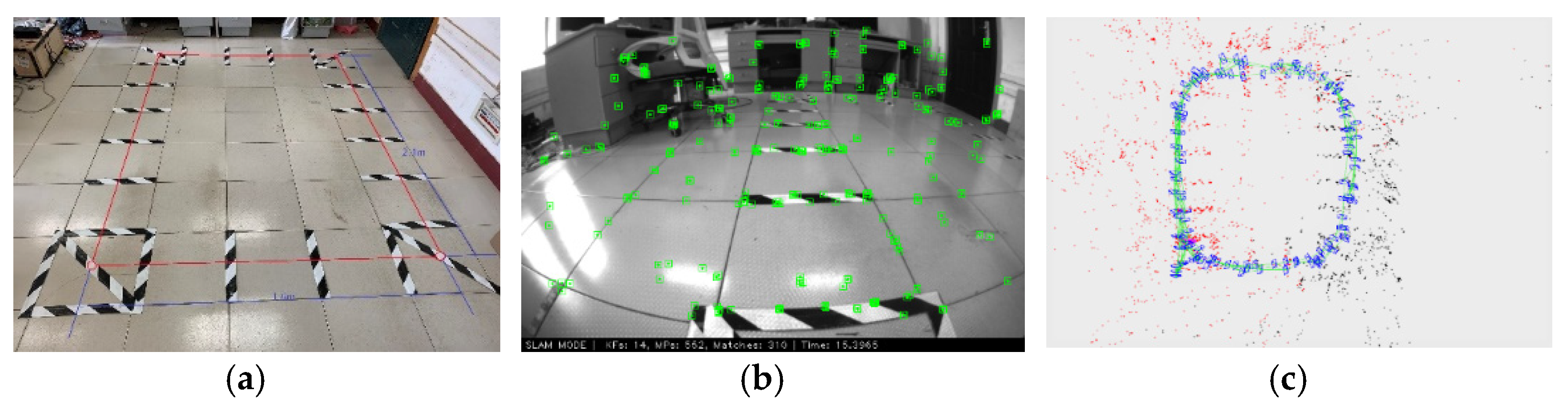
Following the former sections (Section 3.1, Section 3.2 and Section 3.3). Once the accurate gravity vector and gyro bias are acquired, Equation (5) is applied for the pre-integration of positions and velocities, rotate the measurement of acceleration correctly to compensate for the gyro deviation. Subsequently, in consideration of the effect resulting from the accelerometer deviation, the rotation vector ${\mathit{R}}_{WI}$ is also adjusted, which can be described via a two degree of freedom disturbance $\delta \theta$, the Equation (10) can be rewritten as below:

$$\begin{array}{l}{g}_W=R_{WI}Exp(\delta \theta ){\overline{g}}_{I}G\approx R_{WI}{\overline{g}}_{I}G+R_{WI}{(\delta \theta )}^{\wedge }{\overline{g}}_{I}G\\ \begin{array}{cc}& \end{array}=R_{WI}{\overline{g}}_{I}G-R_{WI}{({\overline{g}}_I)}^{\wedge }G\delta \theta \end{array}$$

(17)

with $\delta \theta =[\delta {\theta }_{xy}^T{,0]}^T,\delta {\theta }_{xy}=[\delta {\theta }_x,\delta {\theta }_y{]}^T$.

Therefore, containing the influence of the accelerometer bias, we can get:

$$\begin{array}{l}s·p_{WC}^{i+1}=s·p_{WC}^i+v_{WB}^i\Delta t_{i,i+1}-\frac{1}{2}{R}_{WI}({\overline{g}}_I)\times G\Delta t_{i,i+1}^2\mathsf{\delta }\mathsf{\theta }\\ \begin{array}{ccc}& & \end{array}+R_{WB}^{\mathrm{i}}(\Delta p_{i,i+1}+J_{\Delta p}^a{b}_a)+(R_{WC}^i-R_{WC}^{i+1})p_{CB}+\frac{1}{2}{R}_{WI}{\overline{g}}_{I}G\Delta t_{i,i+1}^2\end{array}$$

(18)

In consideration of the constraints among the three consecutive keyframes, the velocities can be eliminated, and the linear relationship gets as follows:

$$[\lambda (i)\begin{array}{c}\end{array}\phi (i)\begin{array}{c}\end{array}\zeta (i)]\left[\begin{array}{c}s\\ \delta {\theta }_{xy}\\ b_a\end{array}\right]=\psi (i)$$

(19)

Here, we writing N keyframes i, I + 1, I + 2, …, I + N − 1 as 1, 2, 3, …, N for clarity of notation, thus ${\lambda }_{(i)}$, $\phi (i)$, $\zeta (i)$, and $\psi (i)$ are calculated as below:

$$\begin{array}{lll}\lambda (i)& =& (p_{WC}^2-p_{WC}^1)\Delta t_{23}-(p_{WC}^3-p_{WC}^2)\Delta t_{12}\\ \mathsf{\phi }\left(\mathrm{i}\right)& =& {\left[\frac{1}{2}{R}_{WI}({\overline{g}}_I)\times G(\Delta t_{12}^2\Delta t_{23}+\Delta t_{23}^2\Delta t_{12})\right]}_{(:,1:2)}\\ \mathsf{\zeta }\left(\mathrm{i}\right)& =& R_{WB}^2{J}_{\Delta p23}^a\Delta t_{12}+R_{WB}^1{J}_{\Delta v23}^a\Delta t_{12}\Delta t_{23}-R_{WB}^1{J}_{\Delta p12}^a\Delta t_{23}\\ \mathsf{\psi }\left(\mathrm{i}\right)& =& (R_{WC}^2-R_{WC}^1)p_{CB}\Delta t_{23}-(R_{WC}^3-R_{WC}^2)p_{CB}\Delta t_{12}\\ & +& R_{WB}^2\Delta p_{23}\Delta t_{12}+R_{WB}^1\Delta v_{12}\Delta t_{12}\Delta t_{23}-R_{WB}^1\Delta p_{12}\Delta t_{23}+\frac{1}{2}{R}_{WI}{\overline{g}}_{I}G\Delta t_{ij}^2\end{array}$$

(20)

in which ${[]}_{(:,1:2)}$ denotes the top two columns of the matrix. By superimposing all the correlations between three consecutive keyframes (19), the linear system can generate the following equations $A_{3(N-2)\times 6}{X}_{6\times 1}=B_{3(N-2)\times 1}$, which can be solved through the method of singular value decomposition (SVD). In this condition, it is composed of six unknown variables and 3(N-2) equations, and at least four keyframes are required to solve the system.

4. Experiments

The initialization method is applied in an unknown indoor environment with a self-build mobile robot platform. The platform structure is exhibited in Figure 3, the major components include a low-cost VI-camera (MYNT S1030-IR-120), an NVIDIA Jetson TX2, a Xsens MTI-300, and two 12V DC batteries for power supply.

The key parameters of MYNT S1030-IR-120 are shown in

Table 2. Parameters of MYNT camera.

Version	S1030-IR-120
Size	165 mm × 31.5 mm × 31.23 mm
Weight	184 g
Frames per Second	10–60 FPS
Resolution	752 × 480; 376 × 240
FHD	6.0 × 6.0 um
Baseline	120.0 mm
Focal length	2.1 mm
Power dissipation	1–2.7 W @ 5 v DC
IMU frequency	100–500 Hz
Exposure mode	Global shutter
Measuring Depth	0.8–5 m+
Interface	USB 3.0

, it communicates with NVIDIA Jetson TX2 through USB 3.0 interface. In terms of the Xsens MTI-300, it outputs the high-frequency measurements of accelerometers and gyroscopes. In this work, we treat it as a reference system through the post-processing operation. As the low-cost equipment is used to collect datasets, the frequency of the IMU sensor is set to 150 Hz, while the frequency of the camera is set to 10Hz. All of the experiments are implemented by utilizing the computer with i7-9700 CPU (8 cores @3.00 GHz) and 16 GB RAM in the Ubuntu 18.04 + Melodic operating system. The external parameters of the IMU and camera are calibrated via the Kalibr tool [24] in advance which is shown in

Table 3. Camera-IMU joint calibration parameters.

Calibration Parameters
$\mathrm{Extrinsic}: \{T_{CB}$}	${\left[\begin{array}{cccc}0.999967& 0.004309& 0.006957& -0.047774\\ 0.004349& -0.999974& -0.005751& -0.002237\\ 0.006932& 0.005781& -0.999959& -0.021601\\ 0.000000& 0.000000& 0.000000& 1.000000\end{array}\right]}_{4\times 4}$
$\mathrm{Distortion}: \left\{k_1,k_2,p_1,p_2\right\}$	$\{\begin{array}{c}Camera.k1:-0.325639\begin{array}{cc}& Camera.p2:0.000137\end{array}\\ Camera.k2:0.119911\begin{array}{cc}& Camera.p1:0.000158\end{array}\end{array}$

Notes: $T_{CB}$ is the Camera-IMU frames transformation matrix, $k_1,k_2$ is the radial distortion coefficient and $p_1,p_2$ is the tangential distortion coefficient.

.

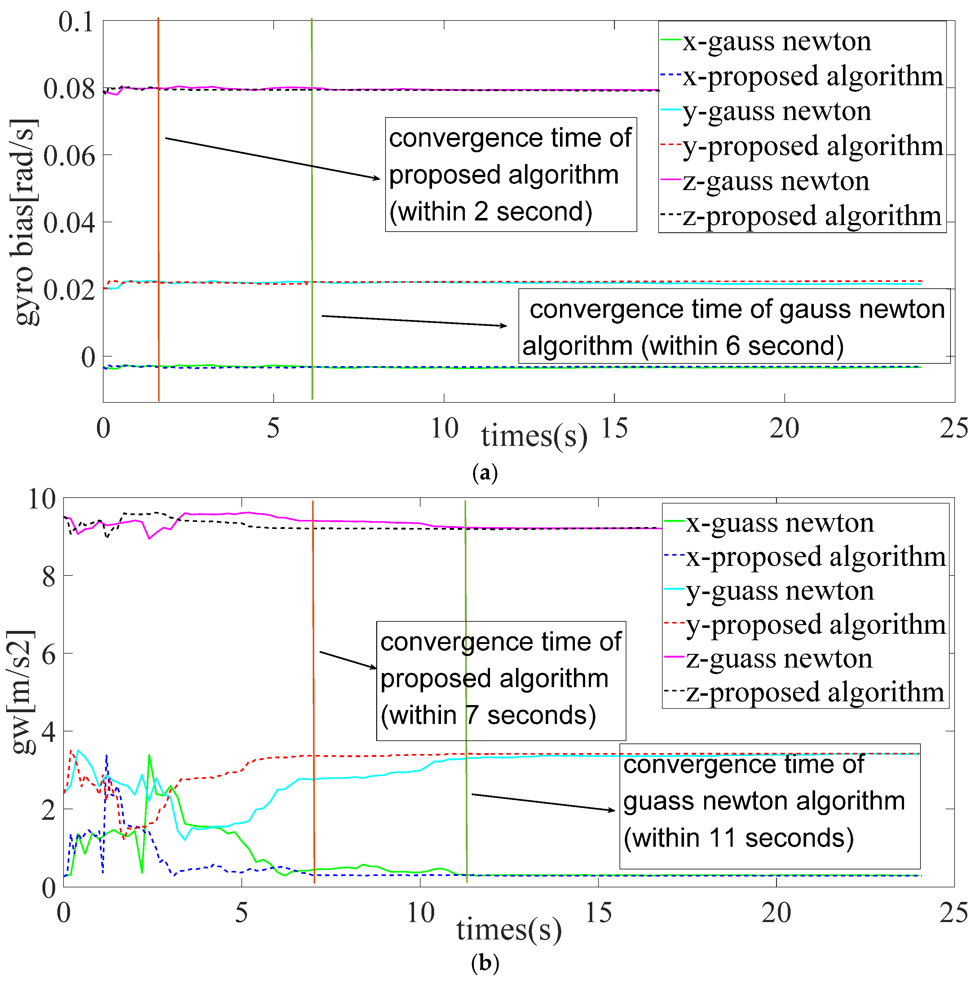
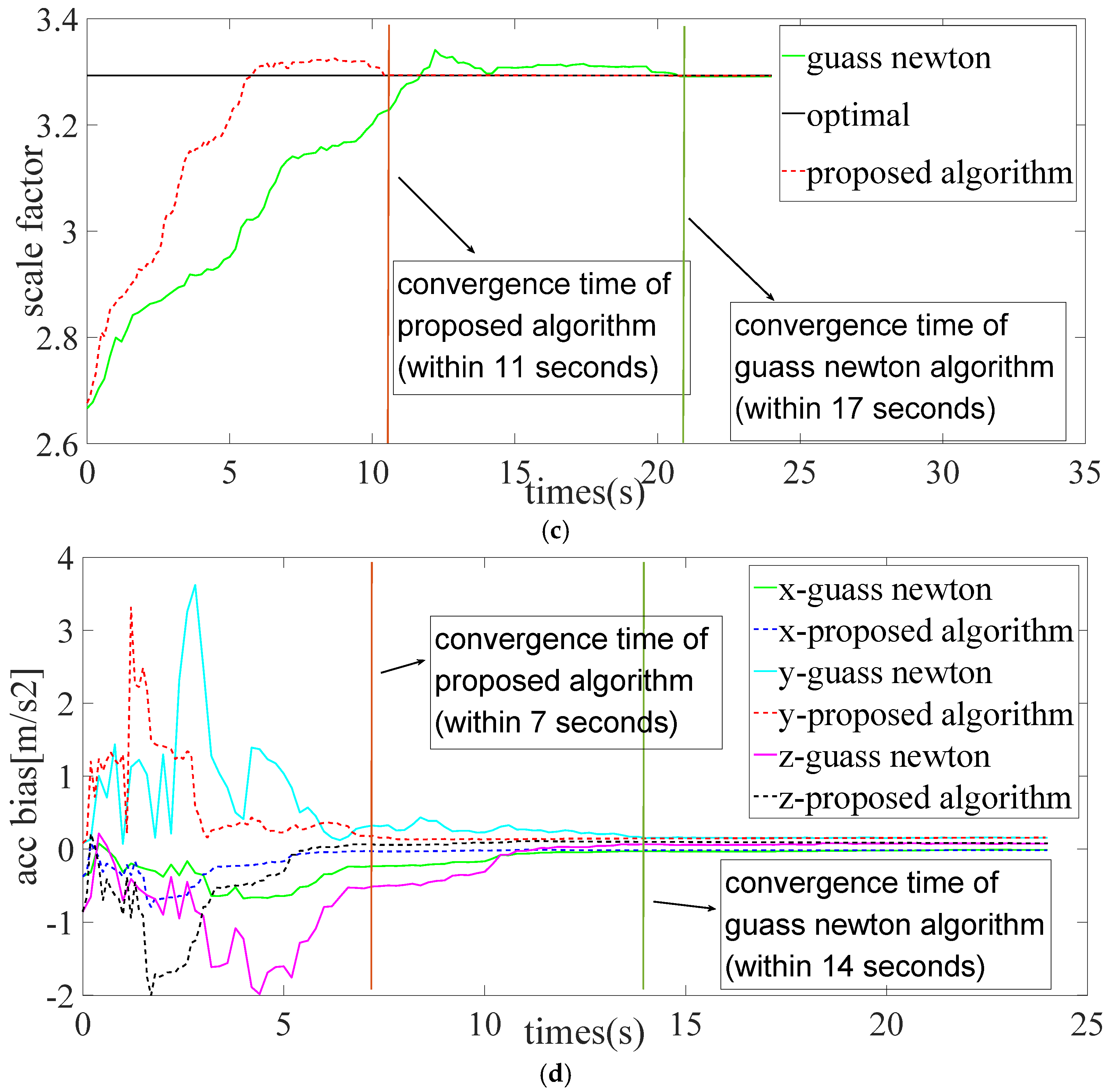
4.1. Evaluation of the Initial Estimation

Our initialization method is first integrated into the VI-SLAM system. To evaluate the algorithms fairly, the original algorithm with the gauss-newton algorithm [19] and the proposed algorithms are detected on the same data set in which the mobile robot is controlled to perform several close-loop movements in the indoor environment. Besides, we only utilized the left camera image to test the performance of the monocular VI-SLAM system. Figure 4a–c shows the example image frame from the laboratory dataset. The comparison results of the initial parameter estimation are shown in Figure 5a–d, it can be known that all estimated variables, containing gravity, gyro deviation, scale factor and accelerometer deviation are converged to the stable values within 2 s to 11 s by using the proposed algorithm (dotted lines), while the gauss newton algorithm (solid lines) is converged within 6 s to 17 s. In particular, as exhibited in the Figure 5a, within 2 s, the gyro bias in x, y, z directions converges to −0.019, 0.023, and 0.081. It is well demonstrated that the iterative method acquired better performance. In Figure 5b,d, the characteristic curves of accelerometer deviation and gravity oscillate seriously within five seconds. This is owing to the mobile robot platform does not show enough excitation to the sensor kit in the slight disturbance and stationary stages, making it difficult to distinguish between gravity vector and accelerometer bias, but the proposed algorithm still has a good performance in convergence speed. In Figure 5c, the visual scale factor is converged 10 s later, and the gauss newton algorithm is converged after 17 s. In general, in the convergence speed, the algorithm is faster than the Gauss–Newton algorithm.

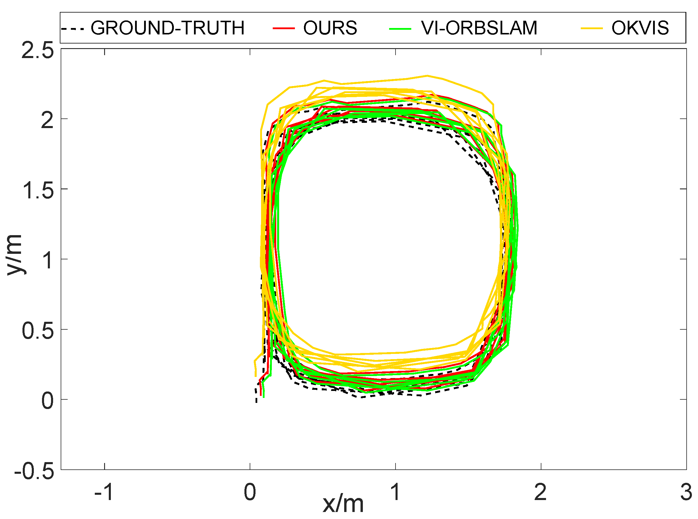
4.2. Evaluation of the Tracking Accuracy and Computational Complexity

In the present section, the property of this algorithm on the VI-SLAM system accuracy was assessed. Similar to the public dataset experiment, when our algorithm is tested on the self-collected dataset, the visual-inertial odometry is utilized as attitude and position feedback. The trajectories are aligned with the reference trajectory, i.e., the measurements of Xsens MTI-300. As exhibited in Figure 6, the dotted line denotes the ground truth trajectories, the yellow line represents the trajectory of OKVIS which is a binocular SLAM method, and the green line and red line represent the trajectories of the gauss-newton based algorithm (i.e., VI-ORBSLAM) and our proposed algorithm, respectively. It can be known that the trajectories can be tracked completely by them, but the three algorithms have different degrees of deviation. Due to the improved initialization process, the trajectory of ours is closer to the ground truth compared with VI-ORBSLAM and OKVIS.

The quantitative evaluation results are obtained through the calculation of Equations (21) and (22). Which the RMSE errors are calculated as follows:

(1)

RMSE error of position:

$$\{\begin{array}{c}RMS{E}_{pos\_x}=\sqrt{\frac{1}{N}{\displaystyle \sum _{k=1}^N{({\overline{x}}_{pos(k)}-x_{pos(k)})}^2}}\\ RMS{E}_{pos\_\mathrm{y}}=\sqrt{\frac{1}{N}{\displaystyle \sum _{k=1}^N{({\overline{y}}_{pos(k)}-y_{pos(k)})}^2}}\\ RMS{E}_{pos\_z}=\sqrt{\frac{1}{N}{\displaystyle \sum _{k=1}^N{({\overline{z}}_{pos(k)}-z_{pos(k)})}^2}}\end{array}$$

(21)

where, $({\overline{x}}_{pos(k)},{\overline{y}}_{pos(k)},{\overline{z}}_{pos(k)})$ denote the estimation of position with x, y, z-axis, $(x_{pos(k)},y_{pos(k)},z_{pos(k)})$ denote the true position with x, y, and z-axis, respectively.

(2)

RMSE errors of orientation:

$$\{\begin{array}{c}RMS{E}_{ori\_x}=\sqrt{\frac{1}{N}{\displaystyle \sum _{k=1}^N{({\overline{x}}_{ori(k)}-x_{ori(k)})}^2}}\\ RMS{E}_{ori\_y}=\sqrt{\frac{1}{N}{\displaystyle \sum _{k=1}^N{({\overline{y}}_{ori(k)}-y_{ori(k)})}^2}}\\ RMS{E}_{ori\_z}=\sqrt{\frac{1}{N}{\displaystyle \sum _{k=1}^N{({\overline{z}}_{ori(k)}-z_{ori(k)})}^2}}\end{array}$$

(22)

where, $({\overline{x}}_{ori(k)},{\overline{y}}_{ori(k)},{\overline{z}}_{ori(k)})$ denote the estimation of orientation with x, y, z-axis, $(x_{ori(k)},y_{ori(k)},z_{ori(k)})$ denote the true orientation with x, y and z-axis, respectively.

As shown in

Table 4. Quantitative RMSE evaluation results of different algorithms.

	VI-ORBSLAM (Monocular)		OKVIS (Binocular)		OURS
	Pos (m)	Ori (°)	Pos (m)	Ori (°)	Pos (m)	Ori (°)
X	0.150	1.356	0.103	1.539	0.091	1.032
Y	0.125	1.165	0.228	1.374	0.115	1.134
Z	0.133	1.987	0.152	3.060	0.123	1.857

the reported value is the median after 10 times of each test. The bold type represents the optimal result. The RMSE errors of position in terms of the VI-ORBSLAM, OKVIS and our proposed algorithm are (0.150, 0.125, 0.133) (m), (0.103, 0.228, 0.152) (m) and (0.091, 0.115, 0.123) (m). Which the position accuracy of ours is increased by (39.3%, 8%, 7.5%) and (11.7%, 49.6%, 19.1%) along x-axis, y-axis, and z-axis in comparison with VI-ORBSLAM and OKVIS, respectively, and The RMSE errors of orientation are (1.356, 1.165, 1.987) (°), (1.539, 1.374, 3.060) (°) and (1.032, 1.134, 1.857) (°), respectively. Which the orientation accuracy of ours is increased by (23.9%, 2.7%, 6.5%) and (32.9%, 17.47%, 39.31%) along x-axis, y-axis, and z-axis, respectively. Obviously, the improvement of position and orientation accuracy in the three-axis is evident. It also well confirms that the proposed initialization method processes a positive role in the positioning accuracy of the monocular VI-SLAM system. In addition, the CPU/memory utilization statistics and pre-frame process time of the three algorithms are also tested, it can be known from

Table 5. Average values of CPU/memory usage and process times.

	VI-ORBSLAM (Monocular)	OKVIS (Binocular)	OURS
CPU Usage (%)	192	175	113
Memory Usage (%)	9.1	7.3	7.0
Process Times (ms)	51	34	29

and Figure 7 that the proposed algorithm has the lowest CPU and Memory usage with the smallest process times of pre-frame.

5. Conclusions and Future Work

In the present work, we put forward a new initialization algorithm for the monocular VI-SLAM system from the perspective of non-linear optimization. Firstly, in the initial stage, the pure vision measurement model of ORB-SLAM is employed to make all the variables visible. Secondly, the frequency of the IMU camera was aligned by IMU pre-integration technology. Thirdly, an improved iterative method is put forward for estimating the initial parameters of IMU faster. Thanks to an improved iterative strategy, our initialization procedure provides high-quality initial seeds which contain gravity vector, gyroscope bias, visual scale as well as accelerometer biases. Besides, a real-world dataset was collected by self-built mobile robots to validate the proposal. The results demonstrate that this algorithm has excellent properties in system positioning accuracy and initial parameter convergence speed than the gauss-newton based algorithm (VI-ORBSLAM) in an indoor environment. A limitation of this strategy is the camera-IMU external parameters are assumed as constant values. The external parameters have an uncertain influence on the initialization results. In future works, we will make additional online estimations of external parameters in the initialization stage to improve the property of the system.

References

1. Lin, Y.; Gao, F.; Qin, T.; Gao, W.; Liu, T.; Wu, W.; Yang, Z.; Shen, S. Autonomous aerial navigation using monocular visual-inertial fusion. J. Field Robot. 2018, 35, 23–51. [Google Scholar] [CrossRef]
2. Bloesch, M.; Omari, S.; Hutter, M.; Siegwart, R. Robust visual inertial odometry using a direct EKF-based approach. In Proceedings of the IEEE/RSJ International Conference on Intelligent Robots and Systems (IROS), Hamburg, Germany, 28 September–2 October 2015; pp. 298–304. [Google Scholar]
3. Taragay, O.; Supun, S.; Rakesh, K. Multi-sensor navigation algorithm using monocular camera, IMU and GPS for large scale augmented reality. In Proceedings of the IEEE International Symposium on Mixed and Augmented Reality, Atlanta, GA, USA, 5–8 November 2012; pp. 71–80. [Google Scholar]
4. Li, P.; Qin, T.; Hu, B.; Zhu, F.; Shen, S. Monocular visual-inertial state estimation for mobile augmented reality. In Proceedings of the IEEE International Symposium on Mixed and Augmented Reality (ISMAR), Nantes, France, 9–13 October 2017; pp. 11–21. [Google Scholar]
5. Fascista, A.; Coluccia, A.; Wymeersch, H.; Seco-Granados, G. Downlink Single-Snapshot Localization and Mapping with a Single-Antenna Receiver. IEEE Trans. Wirel. Commun. 2021, 20, 4672–4684. [Google Scholar] [CrossRef]
6. Ge, Y.; Wen, F.; Kim, H.; Zhu, M.; Jiang, F.; Kim, S.; Svensson, L.; Wymeersch, H. 5G SLAM Using the Clustering and Assignment Approach with Diffuse Multipath. Sensors 2020, 20, 4656. [Google Scholar] [CrossRef] [PubMed]
7. Huang, B.; Zhao, J.; Liu, J. A Survey of Simultaneous Localization and Mapping with an Envision in 6G Wireless Networks. arXiv 2020, arXiv:1909.05214. [Google Scholar]
8. Chen, C.; Zhu, H.; Li, M.; You, S. A Review of Visual-Inertial Simultaneous Localization and Mapping from Filtering-Based and Optimization-Based Perspectives. Robotics 2018, 7, 45. [Google Scholar] [CrossRef] [Green Version]
9. Fascista, A.; Coluccia, A.; Ricci, G. A Pseudo Maximum Likelihood Approach to Position Estimation in Dynamic Multipath Environments. Signal Process. 2021, 181, 707907. [Google Scholar] [CrossRef]
10. Leutenegger, S.; Lynen, S.; Bosse, M.; Siegwart, R.; Furgale, P. Keyframe-based visual-inertial odometry using nonlinear optimization. Int. J. Robot. Res. 2015, 34, 314–334. [Google Scholar] [CrossRef] [Green Version]
11. Murartal, R.; Tardos, J.D. Visual-Inertial Monocular SLAM with Map Reuse. IEEE Robot. Autom. Lett. 2017, 2, 796–803. [Google Scholar] [CrossRef] [Green Version]
12. Von Stumberg, L.; Usenko, V.; Cremers, D. Direct Sparse Visual-Inertial Odometry Using Dynamic Marginalization. In Proceedings of the IEEE International Conference on Robotics and Automation, Brisbane, Australia, 21–25 May 2018; pp. 2510–2517. [Google Scholar]
13. Qin, T.; Li, P.; Shen, S. VINS-Mono: A Robust and Versatile Monocular Visual-Inertial State Estimator. IEEE Trans. Robot. 2018, 34, 1004–1020. [Google Scholar] [CrossRef] [Green Version]
14. Campos, C.; Montiel, J.M.; Tardos, J.D. Inertial-Only Optimization for Visual-Inertial Initialization. In Proceedings of the 2020 IEEE International Conference on Robotics and Automation (ICRA), Paris, France, 31 May–31 August 2020; pp. 51–57. [Google Scholar]
15. Martinelli, A. Closed-form solution of visual-inertial structure from motion. Int. J. Comput. Vis. 2014, 106, 138–152. [Google Scholar] [CrossRef] [Green Version]
16. Kaiser, J.; Martinelli, A.; Fontana, F.; Scaramuzza, D. Simultaneous state initialization and gyroscope bias calibration in visual inertial aided navigation. IEEE Robot. Autom. Lett. 2016, 2, 18–25. [Google Scholar] [CrossRef] [Green Version]
17. Campos, C.; Montiel, J.M.M.; Tardos, J.D. Fast and Robust Initialization for Visual-Inertial SLAM. In Proceedings of the 2019 International Conference on Robotics and Automation, Montreal, QC, Canada, 20–24 May 2019; pp. 1288–1294. [Google Scholar]
18. Burri, M.; Nikolic, J.; Gohl, P.; Schneider, T.; Rehder, J.; Omari, S.; Achtelik, M.W.; Siegwart, R. The EuRoC micro aerial vehicle datasets. Int. J. Robot. Res. 2016, 35, 1157–1163. [Google Scholar] [CrossRef]
19. Murartal, R.; Tardos, J.D. ORB-SLAM2: An Open-Source SLAM System for Monocular, Stereo, and RGB-D Cameras. IEEE Trans. Robot. 2017, 33, 1255–1262. [Google Scholar] [CrossRef] [Green Version]
20. Qin, T.; Shen, S. Robust initialization of monocular visual-inertial estimation on aerial robots. In Proceedings of the IEEE/RSJ International Conference on Intelligent Robots & Systems IEEE, Vancouver, BC, Canada, 24–28 September 2017; pp. 4225–4232. [Google Scholar]
21. Forster, C.; Carlone, L.; Dellaert, F.; Scaramuzza, D. IMU Preintegration on Manifold for Efficient Visual-Inertial Maximum-a-Posteriori Estimation. In Proceedings of the 2015 Robotics: Science and Systems, Rome, Italy, 13–17 July 2015; pp. 1–20. [Google Scholar]
22. Murartal, R.; Montiel, J.M.M.; Tardos, J.D. ORB-SLAM: A Versatile and Accurate Monocular SLAM System. IEEE Trans. Robot. 2015, 31, 1147–1163. [Google Scholar] [CrossRef] [Green Version]
23. Lupton, T.; Sukkarieh, S. Visual-Inertial-Aided Navigation for High-Dynamic Motion in Built Environments without Initial Conditions. IEEE Trans. Robot. 2012, 28, 61–76. [Google Scholar] [CrossRef]
24. Rehder, J.; Nikolic, J.; Schneider, T.; Hinzmann, T.; Siegwart, R. Extending kalibr: Calibrating the extrinsics of multiple IMUs and of individual axes. In Proceedings of the IEEE International Conference on Robotics and Automation, Stockholm, Sweden, 16–21 May 2016; pp. 4304–4311. [Google Scholar]
Figure 1. Coordinate frames of monocular VI−SLAM system.
Electronics 10 03063 g001
Figure 2. The refinement of gravity direction.
Electronics 10 03063 g002
Figure 3. Mobile robot platform: (a) MYNT binocular camera with two global shutter cameras; (b) NVIDIA Jetson TX2 as an onboard computation resource; (c) Xsens MTi-300 as the reference system; (d) batteries with 12V DC power.
Electronics 10 03063 g003
Figure 4. Laboratory scenes and experimental results: (a) the laboratory scene with about 2.4 m long and 1.6 m wide in the indoor environment; (b) the feature-based front end of the system, in which the ORB feature locations are shown in green color; (c) the trajectory of keyframes with a 3D point cloud map.
Electronics 10 03063 g004
Figure 5. Time-varying characteristic curves for initial estimations: (a) the gyroscope bias estimation, “gyro” denotes “gyroscope”; (b) the gravity estimation, “gw” denotes “gravity”; (c) the estimation of the visual scale factor; (d) the estimation of accelerometer bias, “acc” denotes “accelerometer”. The dotted line denotes the algorithm utilizing the improved iterative method, and the solid lines are the outcomes of the algorithm based on Guass–Newton, which is employed in the VI-ORBSLAM system. The convergence time is represented via red and green vertical lines, respectively.
Electronics 10 03063 g005aElectronics 10 03063 g005b
Figure 6. Trajectories comparison with VI-ORBSLAM. The 2D trajectories, VI-ORBSLAM (green line), OKVIS (yellow line), Our system (red line), and ground-truth (dotted line). VI-ORBSLAM adopts gauss-newton algorithm, while our system adopts the proposed algorithm.
Electronics 10 03063 g006
Figure 7. CPU/memory utilization statistics and pre-frame process time summarizing performance. The red color box represents VI-ORBSLAM, the blue color box represents OKVIS, Green color box represents OURS.
Electronics 10 03063 g007