


Performance Evaluation of a UWB Positioning System Applied to Static and Mobile Use Cases in Industrial Scenarios

 ,
,  ,
,  , , and
Abstract
1. Introduction
1.1. Literature Review
1.2. Shortcomings in the Related Work and Paper Contributions
- Extensive empirical performance evaluation of a commercial UWB-positioning system in both static and mobile conditions in a realistic industrial setting.
- Extensive evaluation with focus on static use cases: examining the effects on system accuracy of anchor deployment, tag height, nearby environment, and sample size of the positioning data sets.
- Extensive evaluation with focus on mobile use cases: examining the effects on system accuracy of anchor deployment, and tag position and orientation.
- Extensive statistical analysis addressing the impact of the system’s dynamics on the accuracy.
2. Materials and Methods
2.1. Initial Testing for Fine Tuning of the UWB System Configuration
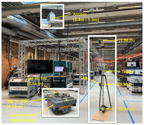
2.2. Measurement Setup for the Static Use Case Evaluation
2.3. Measurement Setup for the Mobile Use Case Evaluation
2.4. Anchor Deployment Configurations
2.5. Accuracy Evaluation Metrics and Data Processing
- is the Euclidean distance between point p and
- p is the ground truth position
- is the ith tag position sample
- is the Euclidean distance between point p and
- p is the ground truth position
- is the average tag position estimated from a total number of N tag position samples, calculated as described in Equation (3):
- is the Euclidean distance between points p and q
- p is the AMR SLAM-based ground truth reference position
- q is the tag position
- offset is the fixed distance between the AMRS SLAM-based ground truth point and the UWB tag position
3. Results
3.1. Static Use Case Evaluation
3.2. Mobile Use Case Evaluation
3.3. Comparison of Static Use Case and Mobile Use Case Accuracies
4. Discussion
4.1. Implications of the Results
4.2. Future Research Directions
5. Conclusions
Author Contributions
Funding
Data Availability Statement
Acknowledgments
Conflicts of Interest
Abbreviations
| AMR | Autonomous Mobile Robot |
| BLE | Bluetooth Low Energy |
| CDF | Cumulative Distribution Function |
| GNSS | Global Navigation Satellite System |
| GPS | Global Positioning System |
| GT | Ground Truth |
| IPS | Indoor Positioning System |
| IR | Infrared |
| IT | Interpolation |
| LiDAR | Light Detection and Ranging |
| LOS | Line-Of-Sight |
| NLOS | Non-Line-Of-Sight |
| PoE | Power-over-Ethernet |
| RF | Radio Frequency |
| RFID | Radio Frequency Identification |
| SD | Standard Deviation |
| SLAM | Simultaneous Localization and Mapping |
| SSP | Samples per Point |
| TDOA | Time Difference of Arrival |
| UWB | Ultra Wideband |
| VLC | Visible Light Communication |
References
- Hofmann-Wellenhof, B.; Lichtenegger, H.; Wasle, E. GNSS—Global Navigation Satellite Systems—GPS, GLONASS, Galileo, and More; Springer: Wien, Austria, 2008. [Google Scholar]
- Rizos, C. Alternatives to current GPS-RTK services and some implications for CORS infrastructure and operations. GPS Solut. 2007, 11, 151–158. [Google Scholar] [CrossRef]
- Subedi, S.; Pyun, J.Y. A Survey of Smartphone-Based Indoor Positioning System Using RF-Based Wireless Technologies. Sensors 2020, 20, 7230. [Google Scholar] [CrossRef]
- Mautz, R. Indoor Positioning Technologies. Ph.D. Thesis, ETH Zurich, Zürich, Switzerland, 2012. [Google Scholar] [CrossRef]
- Álvarez Merino, C.S.; Luo-Chen, H.Q.; Khatib, E.J.; Barco, R. WiFi FTM, UWB and Cellular-Based Radio Fusion for Indoor Positioning. Sensors 2021, 21, 7020. [Google Scholar] [CrossRef]
- Zuo, Z.; Liu, L.; Zhang, L.; Fang, Y. Indoor Positioning Based on Bluetooth Low-Energy Beacons Adopting Graph Optimization. Sensors 2018, 18, 3736. [Google Scholar] [CrossRef] [PubMed]
- Mendoza-Silva, G.; Torres-Sospedra, J.; Huerta, J. A Meta-Review of Indoor Positioning Systems. Sensors 2019, 19, 4507. [Google Scholar] [CrossRef]
- Obeidat, H.; Shuaieb, W.; Obeidat, O.; Abd-Alhameed, R. A Review of Indoor Localization Techniques and Wireless Technologies. Wirel. Pers. Commun. 2021, 119, 289–327. [Google Scholar] [CrossRef]
- Ting, S.; Kwok, S.; Tsang, A.H.; Ho, G.T. The Study on Using Passive RFID Tags for Indoor Positioning. Int. J. Eng. Bus. Manag. 2011, 3, 8. [Google Scholar] [CrossRef]
- Othman, S.N. Node positioning in zigbee network using trilateration method based on the received signal strength indicator (RSSI). Eur. J. Sci. Res. 2010, 46, 048–061. [Google Scholar]
- Brena, R.F.; García-Vázquez, J.P.; Galván-Tejada, C.E.; Muñoz-Rodriguez, D.; Vargas-Rosales, C.; Fangmeyer, J. Evolution of Indoor Positioning Technologies: A Survey. J. Sens. 2017, 2017, 2630413. [Google Scholar] [CrossRef]
- Alarifi, A.; Al-Salman, A.; Alsaleh, M.; Alnafessah, A.; Al-Hadhrami, S.; Al-Ammar, M.; Al-Khalifa, H. Ultra Wideband Indoor Positioning Technologies: Analysis and Recent Advances. Sensors 2016, 16, 707. [Google Scholar] [CrossRef] [PubMed]
- Ridolfi, M.; Van de Velde, S.; Steendam, H.; De Poorter, E. Analysis of the Scalability of UWB Indoor Localization Solutions for High User Densities. Sensors 2018, 18, 1875. [Google Scholar] [CrossRef] [PubMed]
- Gu, Y.; Lo, A.; Niemegeers, I. A survey of indoor positioning systems for wireless personal networks. IEEE Commun. Surv. Tutor. 2009, 11, 13–32. [Google Scholar] [CrossRef]
- Pozyx. Multi Technology RTLS—Indoor & Outdoor. Available online: https://www.pozyx.io (accessed on 1 September 2022).
- Wang, W.; Zeng, Z.; Ding, W.; Yu, H.; Rose, H. Concept and Validation of a Large-scale Human–machine Safety System Based on Real-time UWB Indoor Localization. In Proceedings of the 2019 IEEE/RSJ International Conference on Intelligent Robots and Systems (IROS), Macau, China, 3–8 November 2019; pp. 201–207. [Google Scholar] [CrossRef]
- Barbieri, L.; Brambilla, M.; Trabattoni, A.; Mervic, S.; Nicoli, M. UWB Localization in a Smart Factory: Augmentation Methods and Experimental Assessment. IEEE Trans. Instrum. Meas. 2021, 70, 1–18. [Google Scholar] [CrossRef]
- Stephan, P.; Heck, I.; Krau, P.; Frey, G. Evaluation of Indoor Positioning Technologies under industrial application conditions in the SmartFactoryKL based on EN ISO 9283. IFAC Proc. Vol. 2009, 42, 870–875. [Google Scholar] [CrossRef]
- Ruiz, A.R.J.; Granja, F.S. Comparing Ubisense, BeSpoon, and DecaWave UWB Location Systems: Indoor Performance Analysis. IEEE Trans. Instrum. Meas. 2017, 66, 2106–2117. [Google Scholar] [CrossRef]
- Mimoune, K.M.; Ahriz, I.; Guillory, J. Evaluation and improvement of localization algorithms based on uwb pozyx system. In Proceedings of the 2019 International Conference on Software, Telecommunications and Computer Networks (SoftCOM), Split, Croatia, 19–21 September 2019; IEEE: Piscataway, NJ, USA, 2019; pp. 1–5. [Google Scholar]
- Karaagac, A.; Haxhibeqiri, J.; Ridolfi, M.; Joseph, W.; Moerman, I.; Hoebeke, J. Evaluation of accurate indoor localization systems in industrial environments. In Proceedings of the 2017 22nd IEEE International Conference on Emerging Technologies and Factory Automation (ETFA), Limassol, Cyprus, 12–15 September 2017; pp. 1–8. [Google Scholar] [CrossRef]
- Delamare, M.; Boutteau, R.; Savatier, X.; Iriart, N. Static and Dynamic Evaluation of an UWB Localization System for Industrial Applications. Sci 2020, 2, 23. [Google Scholar] [CrossRef]
- Zwirello, L.; Schipper, T.; Jalilvand, M.; Zwick, T. Realization Limits of Impulse-Based Localization System for Large-Scale Indoor Applications. IEEE Trans. Instrum. Meas. 2015, 64, 39–51. [Google Scholar] [CrossRef]
- Martinelli, A.; Jayousi, S.; Caputo, S.; Mucchi, L. UWB Positioning for Industrial Applications: The Galvanic Plating Case Study. In Proceedings of the 2019 International Conference on Indoor Positioning and Indoor Navigation (IPIN), Pisa, Italy, 30 September–3 October 2019; pp. 1–7. [Google Scholar] [CrossRef]
- Silva, B.; Pang, Z.; Åkerberg, J.; Neander, J.; Hancke, G. Positioning infrastructure for industrial automation systems based on UWB wireless communication. In Proceedings of the IECON 2014—40th Annual Conference of the IEEE Industrial Electronics Society, Dallas, TX, USA, 29 October–1 November 2014; pp. 3919–3925. [Google Scholar] [CrossRef]
- Schroeer, G. A Real-Time UWB Multi-Channel Indoor Positioning System for Industrial Scenarios. In Proceedings of the 2018 International Conference on Indoor Positioning and Indoor Navigation (IPIN), Nantes, France, 24–27 September 2018. [Google Scholar] [CrossRef]
- Silva, B.; Pang, Z.; Åkerberg, J.; Neander, J.; Hancke, G. Experimental study of UWB-based high precision localization for industrial applications. In Proceedings of the 2014 IEEE International Conference on Ultra-WideBand (ICUWB), Paris, France, 1–3 September 2014; pp. 280–285. [Google Scholar] [CrossRef]
- Zwirello, L.; Janson, M.; Zwick, T. Ultra-wideband based positioning system for applications in industrial environments. In Proceedings of the 3rd European Wireless Technology Conference, Paris, France, 27–28 September 2010; pp. 165–168. [Google Scholar]
- Zwirello, L.; Janson, M.; Ascher, C.; Schwesinger, U.; Trommer, G.F.; Zwick, T. Accuracy considerations of UWB localization systems dedicated to large-scale applications. In Proceedings of the 2010 International Conference on Indoor Positioning and Indoor Navigation, Zurich, Switzerland, 15–17 September 2010; pp. 1–5. [Google Scholar] [CrossRef]
- Rodriguez, I.; Mogensen, R.S.; Schjørring, A.; Razzaghpour, M.; Maldonado, R.; Berardinelli, G.; Adeogun, R.; Christensen, P.H.; Mogensen, P.; Madsen, O.; et al. 5G Swarm Production: Advanced Industrial Manufacturing Concepts Enabled by Wireless Automation. IEEE Commun. Mag. 2021, 59, 48–54. [Google Scholar] [CrossRef]
- Leica Geosystems. Leica TS16 Total Station. Available online: https://leica-geosystems.com/products/total-stations/robotic-total-stations/leica-ts16 (accessed on 1 September 2022).
- Mobile Industrial Robots: MiR. MiR200. Available online: https://www.mobile-industrial-robots.com/ (accessed on 1 September 2022).
- Durrant-Whyte, H.; Bailey, T. Simultaneous localization and mapping: Part I. IEEE Robot. Autom. Mag. 2006, 13, 99–110. [Google Scholar] [CrossRef]
- Crețu-Sîrcu, A.L.; Schiøler, H.; Cederholm, J.P.; Sîrcu, I.; Schjørring, A.; Larrad, I.R.; Berardinelli, G.; Madsen, O. Evaluation and Comparison of Ultrasonic and UWB Technology for Indoor Localization in an Industrial Environment. Sensors 2022, 22, 2927. [Google Scholar] [CrossRef]
- Liu, R.; He, Y.; Yuen, C.; Lau, B.P.L.; Ali, R.; Fu, W.; Cao, Z. Cost-effective Mapping of Mobile Robot based on the Fusion of UWB and Short-range 2D LiDAR. IEEE/ASME Trans. Mechatron. 2021. [Google Scholar] [CrossRef]
- Cao, Z.; Liu, R.; Yuen, C.; Athukorala, A.; Ng, B.K.K.; Mathanraj, M.; Tan, U.X. Relative Localization of Mobile Robots with Multiple Ultra-WideBand Ranging Measurements. In Proceedings of the 2021 IEEE/RSJ International Conference on Intelligent Robots and Systems (IROS), Prague, Czech Republic, 27 September–1 October 2021; IEEE: Piscataway, NJ, USA, 2021; pp. 5857–5863. [Google Scholar]


| UWB System | Anchors | Room [m2] | Tag Height [cm] | 2D|3D | GT Points | SPP | Accuracy [cm] | |
|---|---|---|---|---|---|---|---|---|
| [16] | Woku | 8 | 132 | Static N/A Mobile | 2D | 9 | 72 k | <20 |
| [17] | Ubisense | 4 | 110 | 100 | 2D | 25 | 892 | ∼20 (P50) |
| Sewio | 4 | 110 | 100 | 2D | 25 | 104 | ∼55 (P50) | |
| [18] | Ubisense | 4 | 150 | ∼138 | 3D | 8 | - | 7–25 (open) 12–130 (cluttered) |
| [19] | Ubisense | 6 | 336 | 70 | 3D | 72 | 320 | 61 (P50) |
| BeSpoon | 6 | 336 | 70 | 3D | 72 | 40 | 58 (P50) | |
| DecaWave | 6 | 336 | 80 | 3D | 72 | 56 | 39 (P50) | |
| [20] | Pozyx | 4 | 112 | 0–300 | 3D | 9 | 20 | 51–86 |
| [21] | Commercial | 4 | 2760 | - | 2D | 36 | - | 100 (P90) |
| [22] | Decawave | 4–6 | 20 | 70 | 2D | 1 | ∼75 | 1 (static) ∼4–11 (mobile) |
| [23] | Non-commercial | 6 | 95 | 100 | 2D | 32 | 1000 | 3.4 |
| [24] | TimeDomain | 4 | 16 | ∼100 | 2D | 6 | ∼1250 | 2–38 |
| [25] | Decawave | 4 | 60 | ∼100 | 2D | 5 | 1000 | ∼ 5–22 |
| [26] | Decawave | 4 | 70 | - | 2D | 2 | 900 | 10–22 |
| [27] | Decawave | 4 | 60 | ∼100 | 2D, 3D | 5 | 1000 | ∼ 5–40 (2D) 88 (3D) |
| [28] | Simulation | 8 | 1050 | 150 | 3D | 584 | - | 7–13 |
| [29] | Simulation | 8 | 900 | 150–400 | 3D | 500 | - | 7.8 |
| Deployment | Anchor Groups | Evaluated in |
|---|---|---|
| Setup A (Reference) | {1–8} | static and mobile |
| Setup B | {1–4}{1–8} | static and mobile |
| Setup C | {1–3}{1–8} | static |
| Setup D | {1–4}{2,3,4,6}{1–8} | static and mobile |
| Setup E | {1–3}{1–8}{4–8} | mobile |
| Median | 90%-ile | 99%-ile | Samples | min/med/99%-ile | |
|---|---|---|---|---|---|
| [cm] | [cm] | [cm] | SD [cm] | ||
| Anchor deployments | |||||
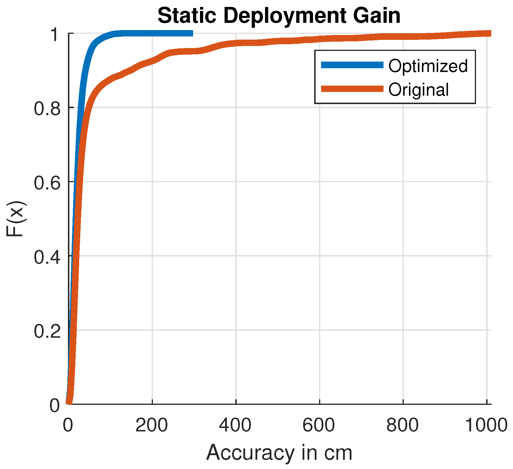
| Original | 21 | 148 | 735 | 833 k | 4/8/45 |
| Optimized | 17 | 40 | 86 | 814 k | 4/7/24 |
| — | |||||
| Environments | |||||
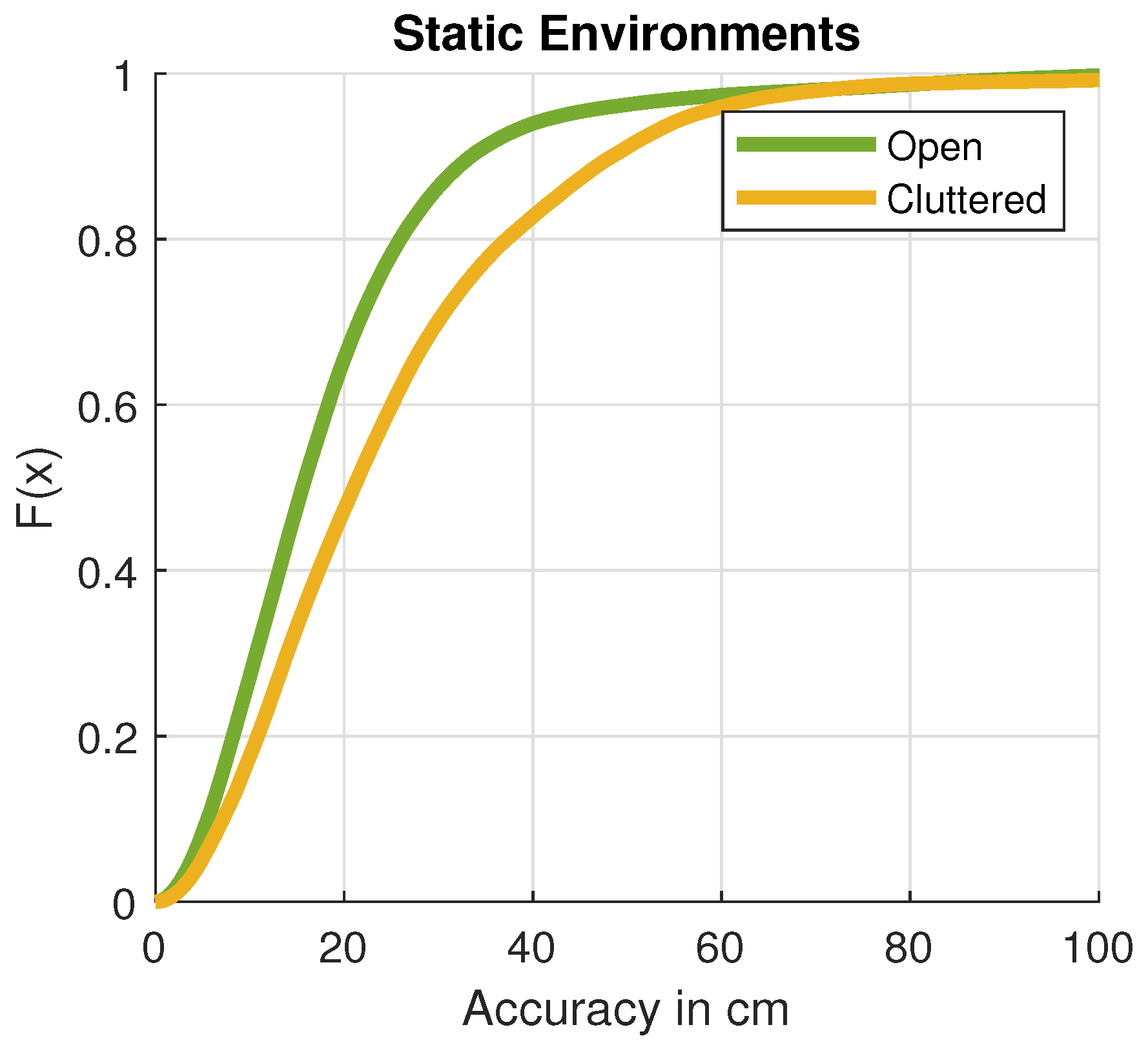
| Open | 16 | 33 | 85 | 529 k | 4/6/12 |
| Cluttered | 21 | 48 | 90 | 285 k | 4/7/40 |
| — | |||||
| Tag heights | |||||
| High | 14 | 28 | 43 | 276 k | 4/6/11 |
| Medium | 19 | 41 | 94 | 267 k | 4/6/16 |
| Low | 20 | 50 | 93 | 270 k | 5/8/40 |
| Aggregation | Median | 90%-ile | 99%-ile | Samples | Median SD |
|---|---|---|---|---|---|
| [cm] | [cm] | [cm] | [cm] | ||
| Non-aggregated | 17 | 40 | 86 | 814 k | 7 |
| 0.1 s (5 samples) | 17 | 40 | 86 | 170 k | 7 |
| 1 s (50 samples) | 17 | 40 | 86 | 17 k | 6 |
| 10 s (500 samples) | 15 | 35 | 86 | 1587 | 3 |
| 90 s (4500 samples) | 14 | 38 | 78 | 216 | - |
| Median | 90%-ile | 99%-ile | Samples | |
|---|---|---|---|---|
| [cm] | [cm] | [cm] | ||
| Anchor deployments | ||||
| Original | 23 | 67 | 153 | 91 k |
| Optimized | 19 | 52 | 102 | 101 k |
| — | ||||
| Tag placements | ||||
| Top | 28 | 55 | 90 | 24 k |
| Left | 14 | 48 | 91 | 20 k |
| Right | 15 | 55 | 112 | 19 k |
| Back | 14 | 39 | 82 | 20 k |
| Front | 14 | 45 | 91 | 19 k |
Publisher’s Note: MDPI stays neutral with regard to jurisdictional claims in published maps and institutional affiliations. |
© 2022 by the authors. Licensee MDPI, Basel, Switzerland. This article is an open access article distributed under the terms and conditions of the Creative Commons Attribution (CC BY) license (https://creativecommons.org/licenses/by/4.0/).
Share and Cite
Schjørring, A.; Cretu-Sircu, A.L.; Rodriguez, I.; Cederholm, P.; Berardinelli, G.; Mogensen, P. Performance Evaluation of a UWB Positioning System Applied to Static and Mobile Use Cases in Industrial Scenarios. Electronics 2022, 11, 3294. https://doi.org/10.3390/electronics11203294
Schjørring A, Cretu-Sircu AL, Rodriguez I, Cederholm P, Berardinelli G, Mogensen P. Performance Evaluation of a UWB Positioning System Applied to Static and Mobile Use Cases in Industrial Scenarios. Electronics. 2022; 11(20):3294. https://doi.org/10.3390/electronics11203294
Chicago/Turabian StyleSchjørring, Allan, Amalia Lelia Cretu-Sircu, Ignacio Rodriguez, Peter Cederholm, Gilberto Berardinelli, and Preben Mogensen. 2022. "Performance Evaluation of a UWB Positioning System Applied to Static and Mobile Use Cases in Industrial Scenarios" Electronics 11, no. 20: 3294. https://doi.org/10.3390/electronics11203294
APA StyleSchjørring, A., Cretu-Sircu, A. L., Rodriguez, I., Cederholm, P., Berardinelli, G., & Mogensen, P. (2022). Performance Evaluation of a UWB Positioning System Applied to Static and Mobile Use Cases in Industrial Scenarios. Electronics, 11(20), 3294. https://doi.org/10.3390/electronics11203294