Article

IPGM: Inertial Proximal Gradient Method for Convolutional Dictionary Learning

1
School of Science, Yanshan University, Qinhuangdao 066004, China
2
School of Information Science and Engineering, Yanshan University, Qinhuangdao 066004, China
3
Hebei Key Laboratory of Information Transmission and Signal Processing, Yanshan University, Qinhuangdao 066004, China
*
Author to whom correspondence should be addressed.
Electronics 2021, 10(23), 3021; https://doi.org/10.3390/electronics10233021
Submission received: 14 October 2021 / Revised: 26 November 2021 / Accepted: 1 December 2021 / Published: 3 December 2021
(This article belongs to the Special Issue Novel Technologies on Image and Signal Processing)

Abstract

:
Inspired by the recent success of the proximal gradient method (PGM) and recent efforts to develop an inertial algorithm, we propose an inertial PGM (IPGM) for convolutional dictionary learning (CDL) by jointly optimizing both an 2 -norm data fidelity term and a sparsity term that enforces an 1 penalty. Contrary to other CDL methods, in the proposed approach, the dictionary and needles are updated with an inertial force by the PGM. We obtain a novel derivative formula for the needles and dictionary with respect to the data fidelity term. At the same time, a gradient descent step is designed to add an inertial term. The proximal operation uses the thresholding operation for needles and projects the dictionary to a unit-norm sphere. We prove the convergence property of the proposed IPGM algorithm in a backtracking case. Simulation results show that the proposed IPGM achieves better performance than the PGM and slice-based methods that possess the same structure and are optimized using the alternating-direction method of multipliers (ADMM).

1. Introduction

Sparse representation is a popular a priori mathematical modeling approach in various signal and image processing applications. Inspired by deep learning-based convolutional operations, convolutional sparse representation is a hot topic at present. In the convolutional sparse representation model, the convolutional dictionary learning (CDL) process plays an important role, but the associated algorithm and convergence proof are difficult problems [1]. CDL involves training dictionaries and estimating codes from multiple signals. In the past decade, the convolutional sparse representation model has achieved impressive results in various applications. The resulting model can achieve excellent performance in image denoising and repair [2], image decomposition [3], image reconstruction [4], medical imaging [5,6], trajectory reconstruction [7], image segmentation [8], superresolution [9], audio processing [10], and other applications. CDL research is a typical interdisciplinary research subject combining mathematics and artificial intelligence. The research results in this field have important theoretical and practical value for a variety of signal and image processing applications. In such a case, a typical assumption is that a signal y N , y = D Γ is a linear combination of columns, also known as atoms. The coefficient Γ M is a sparse vector. A matrix D N × M is called a dictionary. Given y and D , this task of finding its sparsest representation is equivalent to solving the following problem:
min Γ Γ 0   s . t .   y - D Γ 2 ε  
where ε represents the degree of model mismatch or the additive noise intensity. The solutions to such problems can be approximated by greedy algorithms (such as orthogonal matching pursuit (OMP) [11]) or convex formulas (such as basis pursuit (BP) [12]). The task of the developed learning model is to identify the dictionary D that can best represent a set of training signals, called dictionary learning. Several processing methods have been proposed, including K-singular value decomposition (K-SVD) [13], the method of optimal directions (MOD) [14], online dictionary learning [15], and trainlet learning [16]. Unfortunately, many real-world signals, such as images and audio, are high-dimensional signals, making sparse coding computationally challenging. To avoid the curse of dimensionality, high-dimensional signals are decomposed into low-dimensional overlapping signal patches, and sparse coding is performed independently on each signal block [17]. Because of its simplicity and high performance, this method has been widely utilized in a successful manner. However, this method has some limitations that its patch-based process ignores the correlations between patches.
Another option that contrasts with this local paradigm is a global model [18] called the convolutional sparse representation model. The input signal is represented as the superposition of the convolutional results of some local atoms and sparse feature mappings. The problem is solved by applying a specific structure to the global dictionary involved. In particular, the dictionary in this model is constrained to a banded circulant matrix formed by atomic cascades, which is called convolutional sparse representation.
The convolutional sparse representation model is as follows:
y = D Γ = m d m γ m
where a signal y N , the banded global convolutional dictionary D N × N M is composed of a local convolutional dictionary filter, { d m } m = 1 M n , a cyclic shift composed of the atom D L n × M , and the coding coefficient Γ N M is composed of { γ i } i = 1 M , where γ i N .
This work proposes a theoretical analysis of a new global convolutional sparse representation model, which guarantees the local sparsity metric. The convolutional dictionary directly determines translation invariance to compensate for the problem that the correlations between adjacent signal patches are ignored. By using this convolutional dictionary structure, convolutional sparse coding (CSC) and CDL have arisen. For the convenience of calculation, the 1 norm of the coefficient is used instead of the 0 norm, and a spherical constraint is used for the dictionary instead of the sphere constraint. Several convex and relaxed CDL algorithms have been proposed [19,20,21,22]. They mainly utilize the alternating-direction method of multipliers (ADMM) solver based on the Fourier domain. However, the ADMM loses its connection to the patch-based processing paradigm that is widely used in many signal and image processing applications [23].
Papyan proposed a new convex relaxation algorithm [23] via slice-based dictionary learning (SBDL), where the sum of the slices forms the signal patches. The developed algorithm is an ADMM solver based on the signal domain. It adopts a local point of view and trains a convolutional dictionary only according to the local calculation of the signal domain. It runs on local slices and faithfully solves the problem of global convolutional sparse coding. This local–global method and its resulting decomposition follow a recent work [18] that compared it with the Fourier-based method. The SBDL algorithm is easy to implement, is intuitive, achieves the most advanced performance, and converges faster than other approaches. Moreover, it provides a better model that can naturally allow a different number of nonzero values to be contained in each spatial location according to the local signal complexity. The ADMM parameters strongly depend on the given problem. Although its corresponding pursuit algorithm can be proven to be convergent, when the convolutional dictionary is iteratively updated in the ADMM algorithm, it is difficult to prove the convergence of the tracking algorithm [24].
The convex relaxation and ADMM-based optimization algorithm produce a nonsparse coding solution, and it is challenging to prove the algorithmic convergence [25]. In addition, in nonconvex optimization, the greedy algorithm for CDL problems has a high computational cost, poor performance, and convergence proof difficulty [26]. Chun and Fessler [27] recently proposed an algorithm that could achieve full convergence. However, the method involves approximate convex constraints, and its overall performance is slightly better than that of the ADMM. The CDL problem is essentially a nonconvex and nonsmooth optimization problem, as shown in the following formula, making it difficult to propose an optimization algorithm and prove its convergence.
arg min { d m } , { γ l , m } 1 2 l m = 1 M d m γ l , m y l 2 2 + λ 1 l m = 1 M Ω 1 ( γ l , m ) + λ 2 m = 1 M Ω 2 ( d m )
where λ i , i = 1 , 2 is the equilibrium coefficient and Ω i , i = 1 , 2 is the nonconvex constraint of the coefficient and the convolutional dictionary. For example, in a case with typical nonconvex constraints, Ω 1 ( x ) = x 0 is a zero norm, and Ω 2 ( d m ) = d m 2 2 = 1 is a spherical constraint.
Peng [28] realized the joint and direct optimization of the CDL problem under a nonconvex and nonsmooth optimization scheme and proposed a forward–backward splitting algorithm based on the Fourier domain. The developed approach is better than the ADMM algorithm. To be more precise, the forward step involves estimating the smooth part of the objective function through a partial gradient. In contrast, the backward step counts the degree of nonsmoothness of the objective function through its proximal operator. Peng proved the convergence of the solution sequence of the proposed algorithm by using the semialgebraic property of reference [29] and the Kurdyka–Lojasiewicz (KL) property. Peng [28] used the gradient descent algorithm in the dictionary and coding process. Although this dramatically reduces the computational complexity of the overall algorithm, in theory, the gradient descent algorithm can only guarantee that it will reach the lowest local point, not the lowest global point. Many minimum points are contained in many complex functions. In many cases, we can only obtain the optimal local solution by using the gradient descent method and not the optimal global solution. In addition, when the sample size of the given dataset is large, the convergence speed of the gradient descent algorithm is slow.
Polyak [30] proposed the heavy-ball method that an inertia term is added to the standard gradient descent method. This method has a faster convergence rate than the standard gradient method based on an unchanging number of required calculations. Peter Ochs [31] applied this method to a convex optimization scheme. He proposed an iPiano algorithm combining an inertia term and a forward–backward splitting frame to address minimization problems consisting of differentiable (possibly nonconvex) and convex (possibly nondifferentiable) functions. These problems were strictly analyzed, and the global convergence of the function values and parameters was determined. Simultaneously, the efficiency of convergence was greatly improved. We will apply this inertia term algorithm to the CDL problem.
In this paper, an inertial forward–backward splitting algorithm is proposed for the CDL problem. The convergence of the algorithm is given and proven. The optimal convergence rate is derived. Finally, a large number of experiments show that the proposed algorithm has high efficiency and effectiveness.
The rest of this article is organized as follows. In Section 2, we introduce some related knowledge. In Section 3, the inertia forward and backward splitting algorithm is proposed to restate the CDL problem. In Section 4, the complexity of the proposed algorithm is analyzed. In Section 5, the convergence of the proposed algorithm is analyzed and proven. The convergence rate of the proposed algorithm is derived in Section 6. In Section 7, the performance of the proposed algorithm is evaluated through experiments and compared with other existing methods. Section 8 summarizes the full text.

2. Related Knowledge

2.1. Convex CDL in the Time Domain via Local Processing

The CSC model [19] assumes that a global signal y N can be decomposed as
y = D Γ = i = 1 N P i T D L α i
The matrix D N × N M is a banded convolutional dictionary. This matrix consists of all shifted versions of a local dictionary D L n × m whose columns are atoms. L represents the initial of the word “local.” The global sparse vector Γ N M can be decomposed into N non-overlapping, m-dimensional local sparse vectors { α i } i = 1 N , where α i M are called needles. The operator P i T places D L α i in the ith position of the signal. The above formula can be used to obtain sparse coefficients using the basic pursuit problem, as shown below:
min { α i } i = 1 N 1 2 y i = 1 N P i T D L α i 2 2 + λ i = 1 N α i 1
Papyan et al. [23] proposed slice-based local processing and defined s i = D L α i as the ith slice. Unlike other existing works in signal and image processing, which train a dictionary in the Fourier domain, they defined the learning problem based on the constructed slices, and CDL was carried out in the signal domain via local processing. Through local processing in the original signal domain, the global problem was solved completely. The global signal y l can be rewritten as y = i = 1 N P i T s i .
The ADMM algorithm is used to solve the problem of minimizing the following augmented Lagrangian problem:
min D L , { α i } i = 1 N , { s i } i = 1 N , { u i } i = 1 N 1 2 y i = 1 N P i T s i 2 2 + i = 1 N ( λ α i 1 + ρ 2 s i D L α i + u i 2 2 )
where { u i } i = 1 N are the dual variables that satisfy the given constraint. ρ is the Lagrangian coefficient. References [23,24] call this method the SBDL algorithm.
In the SBDL algorithm, the CDL problem is transformed into a traditional dictionary learning problem solved by the K-SVD algorithm [13] or other dictionary learning algorithms. The sparse coding process is based on the ADMM algorithm for updating, and each coding update is regarded as a least absolute shrinkage and selection operator (LASSO) problem, which is solved by the least-angle regression and shrinkage (LARS) algorithm. The ADMM is used to solve the coding problem, which increases the numbers of auxiliary variables, calculations and redundant iterations. In addition, different solving methods are used to update dictionary and codes, which makes it difficult to prove the convergence of the algorithm.

2.2. Forward–Backward Splitting

Splitting algorithms for convex optimization problems usually originate from the proximal point algorithm [32]. The proximal point algorithm is very general, and the results regarding its convergence affect many other algorithms. However, in practice, an iteration of the computational algorithm can be as tricky as the original problem. The strategy to solve this problem involves splitting approaches such as the Douglas–Rachford method, several primal-dual algorithms, and forward–backward splitting.
Forward–backward splitting schemes have been used to solve a variety of problems in recent years. For example, forward–backward splitting algorithms are used to solve normal problems [33], to find generalized Nash equilibrium [34], to solve linear constraint problems [35], or to analyze related function problems in Banach space [36,37]. In particular, it is appealing to generalize forward–backward splitting schemes to nonconvex problems. This is due to their simplicity and simpler formulations in some exceptional cases, such as the gradient projection method, where the backward step is a projection onto a set. The backward step of the forward–backward algorithm studied in [28] is the solution of a proximal term of a nonconvex function.
The goal of a forward–backward splitting framework is to solve the following forms of an optimization problem:
arg min x f ( x ) + g ( x )
However, when a large amount of data is processed, even if misestimation is not considered during processing, the processing result of the forward–backward splitting algorithm becomes inaccurate. In this paper, the original algorithm is improved to increase the accuracy and reduce the induced error.

2.3. Inertia Item

Polyak studied a multistep scheme for the accelerated gradient method in [30] and proposed the heavy-ball method for the first time. Unlike the usual gradient method, this approach adds an inertia term, which is calculated by the difference between the values obtained during the previous two iterations. Compared with the standard gradient method, this method can accelerate the convergence speed of the algorithm while keeping the cost of each iteration unchanged. In addition, this method can obtain the optimal convergence rate without additional knowledge.
The inertia term of the heavy-ball method was first applied to the minimization of differentiable convex functions, and then it was extended to subdifferential convex functions. Later, the heavy-ball method was used for forward–backward splitting [37,38]. Recently, it has been frequently applied to the minimization of nonconvex functions. In [39,40], the inertia term was introduced into the nonconvex optimization problem to improve the convergence speed. Refs. [31,41] used an inertia term to develop a nonconvex optimization CDL scheme. The authors of [31] aimed to minimize problems composed of differentiable (possibly nonconvex) and convex (possibly nondifferentiable) functions. The iPiano algorithm was proposed by combining forward–backward splitting with an inertia term. The global convergence of the function values and parameters was determined. In [41], an inertial version of the proximal alternating linearization minimization (PALM) algorithm was proposed, and its global convergence to the critical point of the input objective function was proven.

3. Proposed IPGM Algorithm

The CDL problem to be solved via local processing is given as follows:
arg min { α i } i = 1 N , D L 1 2 l i = 1 N P i T D L α l , i y l 2 + λ 1 l ( i = 1 N Ω 1 ( α l , i ) ) + λ 2 Ω 2 ( D L )
D L is the local convolutional dictionary, which has n rows and m columns. α l , i , which has m rows, is the sparse coding of each component i of each sample l. P i T , which has N rows and n columns, is the operator that puts D L α l , i in the ith position and pads the rest of the entries with zeros. y l is the observed signal. has different meanings; when the interior is a vector, represents the 2 -norm, and when the interior is a matrix, represents the Frobenius norm. λ 1 and λ 2 are hyperparameters. Ω 1 is the sparse constraint imposed on the column vectors with the 0 norm or 1 norm, which is defined as follows: Ω 1 ( x ) = x 0 or Ω 1 ( x ) = x 1 . Ω 2 is the indicator function of unit-norm sphere.
To solve the above convex or nonconvex CDL optimization problem (8) via local processing, we use the inertial forward-backward splitting framework. An inertial forward-backward splitting algorithm via local processing called the inertial proximal gradient method (IPGM) algorithm is proposed.
To form the objective function of the proposed CDL optimization problem via local processing with the developed framework, based on the proposed Equation (8), supposing that x = ( D L t , { α l , i t } ) , { x t } can be generated by iteratively implementing the following equation:
x t + 1   p r o x ( ( x t η t f ( x t ) + ξ t ( x t x t 1 ) )
where prox refers to the proximal mapping operation.
f and g are, respectively defined as follows:
f ( D L , { α l , i } ) = 1 2 l i = 1 N P i T D L α l , i y l 2
g ( D L , { α l , i } ) = l ( i = 1 N λ 1 Ω 1 ( α l , i ) ) + λ 2 Ω 2 ( D L )
To generate the sequence { x t } = { D L t , { α l , i t } } using iterative Equation (9) based on inertial forward-backward splitting, we first need to derive the gradient of f and the proximal mapping of g .
Since f is a function of the composite variable x or ( D L , { α l , i } ) , we define the gradient of f as follows:
f : = { D L f , { α l , i f } }
D L f and α l , i f can be computed as follows:
D L f = l i = 1 N ( P i ( i = 1 N P i T D L α l , i y l ) α l , i T )
α a , b f = D L T P b ( i = 1 N P i T D L α a , i y a )
To show the result of the descent process, we use an intermediate variable ( D L t + 1 / 2 , { α l , i t + 1 / 2 } ) :
D L t + 1 / 2 : = D L t η t D L f + ξ t ( D L t - D L t - 1 )
α l , i t + 1 / 2 : = α l , i t η t α l , i f + ξ t ( α l , i t - α l , i t - 1 )
where η t is a step size or descent parameter and ξ t is an inertial parameter. Therefore, we compute the proximal mapping of g at ( { D L t + 1 / 2 } , { α l , i t + 1 / 2 } ) as follows:
( D L t + 1 , { α l , i t + 1 } ) = p r o x η t g ( D L t + 1 / 2 , { α l , i t + 1 / 2 } ) = ( { p r o x η t λ 2 Ω 2 ( D L t + 1 / 2 ) } , { p r o x η t λ 1 0 ( α l , i t + 1 / 2 ) } )
The function prox refers to the proximal mapping operation, which is defined with the following form:
p r o x η p ( u ) = arg min v 1 2 η u v 2 + p ( v )
Furthermore, in the inertial forward-backward splitting framework, to accelerate the convergence rate, we propose using η t to fit the local curvature of f in each iteration and capturing the local curvature f by estimating the local Lipschitz constant of the CDL problem via local processing. This constant is defined as follows:
L t = f ( x t ) f ( x t 1 ) 2 x t x t 1 2
However, the direct derivation of η t from L t does not satisfy the convergence requirement. It is suggested to insert a backtracking scheme in the inertial forward-backward splitting framework to restore its convergence.
We introduce a sequence { τ t } , where τ t > 1 holds for all t , to represent the adaptive parameter such that the sequence { x t } satisfies the following equation:
f ( x t + 1 ) f ( x t ) + f ( x t ) , x t + 1 x t + τ t L t 2 x t + 1 x t 2
We assume that each step size η t is maintained by τ t using the inequality 0 < η t < ( 1 / ( τ t L t ) ) and that (20) can be reformulated as follows:
f ( x t + 1 ) = f ( D L t + 1 , { α l , i t + 1 } ) f ( x t ) + f ( x t ) , x t + 1 x t + 1 2 η t x t + 1 x t 2                             = f ( D L t , { α l , i t } ) + p , q [ α p , q t + 1 ( α p , q f ) ( D L t , { α l , i t } ) + 1 2 η t Γ r ( ( α p , q t + 1 α p , q t ) T ( α p , q t + 1 α p , q t ) ) ]                             + D L t + 1 ( D L f ) ( D L t , { α l , i t } ) + 1 2 η t Γ r ( ( D L t + 1 D L t ) T ( D L t + 1 D L t ) )
where stands for the Hadamard product.
We present the IPGM algorithm that solves the proposed CDL problem via local processing using inertial forward–backward splitting in Algorithm 1.
Algorithm 1 The IPGM algorithm for solving the proposed CDL problem via local processing
Input: initial dictionary D L 0 ; initial dictionary D L - 1 = D L 0 ; initial coefficients map { α l , i 0 } ; initial coefficient maps { α l , i - 1 } = { α l , i 0 } ; adaptive parameter τ > 1 ; choose c 1 > 0 close to 0; inertial parameter ξ 0 [ 0 , 1 2 ) ; and descent parameter 1 < η 0 < ( 1 2 ξ 0 ) / τ L , where L is the Lipschitz constant of f .
Output: learned dictionary D L t ; learned coefficients { α l , i t } ;
1: Initialization: t 0
2: repeat
3:               if  t < 2 , then
4:                                η t η 0 , ξ t ξ 0
5:                else
6:                               compute L t using Equation (19)
7:                                  η t 1 L t
8:               end if
9:                                k     0
10:               repeat
11:                               compute D L f and α l , i f using Equations (13) and (14)
12:                               compute ( D L t + 1 / 2 , { α l , i t + 1 / 2 } ) using Equations (15) and (16)
13:                               update ( D L t + 1 , { α l , i t + 1 } ) using Equation (17)
14:                                τ t τ k
15:                                η t η t τ
16:                                k k + 1
17:               until Equation (21) is satisfied
18:                                  η t c 1 ,   ξ t 0
19:                                  δ t : = 1 2 η t τ t L t 2 ξ t 2 η t
20:                                 γ t : = 1 2 η t τ t L t 2 ξ t η t
21:       until    δ t γ t c 1 and ( δ t )   t = 0 is monotonically decreasing
22:        t t + 1
23: until convergence
24: return { { D L t } , { α l , i t } }

4. Computational Complexity Analysis

The computational complexity of our algorithms is discussed as follows. We assume the following. N is the signal dimension. I is the number of signals. n is the patch size. m is the number of filters. k is the maximal number of nonzeros in a needle α l , i , which is very sparse k m . C is the number of backtracking loops, which is usually very small. The convolution is performed by the local processing operation. The operation P i T is only an operator of a column to an image.
The dominant computational complexity of the signal reconstruction performed by the local processing operation is approximately O ( I N n k ) . The computation of the signal residual requires O ( I N ) operations. Neglecting some minor factors, the computational complexity of the gradient of needles and dictionary performed by the local processing operation is effectively O ( I N n m ) and O ( I N n k ) , respectively. In addition, the inertia term includes an addition and a multiplication for each iteration which is negligible.

5. Proof of the Convergence of Algorithm 1

Before describing the convergence theorem, let us analyze the relevant lemmas and hypotheses.
Lemma 1.
(The abstract convergence result for KL functions) This convergence result is based on three abstract conditions for a sequence ( z t ) t : = ( x t ,   x t 1 ) t   2 N , x t N ,   x t 1 N . We fix two positive constants a > 0 and b > 0 and consider a proper lower semicontinuous function F :   2 N   { } . Then, the conditions for ( z t ) t are as follows:
(H1) For each k , it holds that
F ( z k + 1 ) + a x k x k 1 F ( z k )
(H2) For each k , there exists a w k + 1 F ( w k + 1 ) such that
w k + 1 b 2 ( x k x k 1 + x k + 1 x k )
(H3) There exists a subsequence ( z k j ) j such that
z k j z ˜   a n d   F ( z k j ) F ( z ˜ )   a s   j
When F is a KL function and H1, H2, and H3 are satisfied, F satisfies the convergence result.
Lemma 2.
For all n 0 , δ t γ t , ξ t [ 0 , 1 2 ) , and η t ( 1 2 ξ t ) / τ t L t . Furthermore, given L t > 0 , there exists a pair of parameters η t and ξ t such that ( δ t ) t = 0 is monotonically decreasing.
Proof of Lemma 2.
By the algorithmic requirements,
δ t = 1 2 η t τ t L t 2 ξ t 2 η t 1 2 η t τ t L t 2 ξ t η t = γ t 0
The upper bounds for ξ t and η t are obtained by rearranging γ t c 1 to ξ t ( 1 η t τ t L t 2 η t c 1 ) / 2 and η t ( 1 2 ξ t ) / ( 2 c 1 + τ t L t ) , respectively.
The last statement follows by incorporating the descent property of δ t   . Let δ 1 c 1 be chosen initially. Then, the decent property of ( δ t ) t = 0 requires one of the equivalent statements below
δ t 1 δ t δ t 1 1 2 η t τ t L t 2 ξ t 2 η t η t ( 1 ξ t ) / ( 2 δ t 1 + τ t L t )
to be true. An upper bound on η t is obtained by
γ t c 1 η t 1 2 ξ t 2 c 1 + τ t L t
Consider the condition for a nonnegative gap between the upper and lower bounds of η t :
1 2 ξ t 2 c 1 + τ t L t 1 ξ t 2 δ n 1 + τ t L t 0 2 δ n 1 + τ t L t 2 c 1 + τ t L t 1 ξ t 1 2 ξ t
Defining b : = ( 2 δ + τ t L t ) / ( 2 c 1 + τ t L t ) 1 , it is easily verified that there exists ξ t [ 0 , 1 2 ) satisfying the equivalent condition
b 1 2 b 1 ξ t
As a consequence, the existence of a feasible η t follows, and the decent property for δ t holds. □
Proposition 1.
(a) The sequence ( H δ t ( x t , x t 1 ) ) n = 0 is monotonically decreasing and thus convergent. In particular, it holds that
H δ t + 1 ( x t + 1 , x t ) H δ t ( x t , x t 1 ) γ t Δ t 2
(b) It holds that n = 0 Δ t 2 < , and thus, lim t Δ t = 0 .
Proof of Proposition 1.
(a) For a more convenient notation, we abbreviate h = f + g in the IPGM algorithm for the nonconvex nonsmooth CDL problem via local processing; this does not mean that the value of the function drops, so we construct a function H δ ( x ,   y ) = h ( x ) + δ x y 2 ,   δ . Note that for x = y , H δ ( x ,   y ) = h ( x ) .
We show below that H δ ( x ,   y ) satisfies the convergence requirement. In the inertial forward–backward splitting framework, the sequence { x t } is generated by iteratively implementing Equation (9).
Notably, in the IPGM algorithm, the function f satisfies the adaptive descent formula in (20).
The function g is a nonconvex, nonsmooth, and proper closed function. Combining the iterative mapping of the sequence { x t } in the inertial forward–backward splitting framework and the definition of the proximal operator, we can obtain
1 2 η t x t + 1 ( x t η t f ( x t ) + ξ t ( x t x t 1 ) ) 2 + g ( x t + 1 )     1 2 η t x t ( x t η t f ( x t ) + ξ t ( x t x t 1 ) ) 2 + g ( x t )
Thus, this simplifies to
g ( x t + 1 ) + 1 2 η t x t + 1 x t 2 + 1 η t x t + 1 x t , η t f ( x t ) ξ t ( x t x t - 1 ) g ( x t )
Now, using (20) and (29) by summing both inequalities, it follows that
h ( x t + 1 ) h ( x t ) ( 1 2 η t τ t L t 2 ) x t + 1 x t 2 + ξ t η t x t + 1 x t , x t x t 1 h ( x t ) ( 1 2 η t τ t L t 2 ξ t 2 η t ) x t + 1 x t 2 + ξ t 2 η t x t x t 1 2
where the second line follows from   2 A , B A 2 2 + B 2 2 for vectors A , B N . Then, a simple rearrangement of the terms yields:
h ( x t + 1 ) + δ t x t + 1 x t 2 h ( x t ) + δ t x t x t 1 2 γ t x t x t 1 2
which establishes (27) as δ t is monotonically decreasing. The sequence ( H δ t ( x t , x t 1 ) ) n = 0 monotonically decreases if and only if γ t 0 , which is confirmed by the algorithmic requirements. By assumption, h is bounded from below by some constant h _ > ; hence, ( H δ t ( x t , x t 1 ) ) n = 0 converges.
(b) Summing (27) from t = 0 , , T yields (note that H δ t ( x 0 , x 1 ) = h ( x 0 ) )
t = 0 T r t Δ t 2 t = 0 T H δ t ( x t , x t 1 ) H δ t + 1 ( x t + 1 , x t ) = h ( x 0 ) H δ T + 1 ( x T + 1 , x T ) h ( x 0 ) h _ <
Letting T tend to , it can be seen from (32) that lim t T γ t Δ t 2 = 0 since γ T c 1 > 0 implies the above statement. □
Proposition 2.
(a) The sequence ( h ( x t ) ) t = 0 converges.
(b) There exists a convergent subsequence ( x t k ) k = 0 .
(c) Any limit point x : = l i m k x t k is a critical point of h ( x ) , and h ( x t k ) h ( x ) as k .
Proof of Proposition 2.
(a) This follows from the squeeze theorem as for all t 0 , the following holds:
H δ t ( x t ,   x t 1 )     h ( x t )     H δ t ( x t ,   x t 1 )
and due to Propositions 1(a) and (b),
lim t H δ t ( x t ,   x t 1 ) = lim t H δ t ( x t ,   x t 1 ) 2 δ t Δ n 2 = lim t H δ t ( x t ,   x t 1 )
(b) By Proposition 1(a) and the fact that H δ 0 ( x 0 ,   x 1 ) = h ( x 0 ) , it is clear that the whole sequence ( x t ) t = 0 is contained in the level set { x N   :   h     h ( x )     h ( x 0 ) } , which is bounded due to the coercivity of h and because h = inf x N   h ( x ) > . Using the Bolzano-Weierstrass theorem, we deduce the existence of a convergent subsequence ( x t k ) k = 0 .
(c) To show that each limit point x = l i m j x t j is a critical point of h ( x ) , we recall that the subdifferential is closed. We define
ς j : = x t j x t j + 1 η t j   f ( x t j ) + ξ t j η t j   ( x t j x t j 1 ) + f ( x t j + 1 ) .
Then, the sequence ( x t j ,   ς j ) G r a p h ( h )   : = { ( x ,   ς ) N × N | ς h ( x ) } . Furthermore, it holds that x = l i m j x t j , and due to Proposition 1(b), f is Lipschitz-continuous, and
ς j 0   1   η t j   Δ n j + 1 + ξ t j η t j   Δ n j + f ( x t j + 1 ) f ( x t j )
It holds that l i m j ς j = 0 . It remains to be shown that l i m j h ( x t j ) = h ( x ) . By the closure property of the subdifferential h , ( x , 0 ) G r a p h ( h ) , which means that x is a critical point of h .
According to the iterative mapping (Equation (9)) of the sequence { x t } in the inertial forward-backward splitting framework, we can obtain:
1 2 η t x t + 1 ( x t η t f ( x t ) + ξ t ( x t x t 1 ) ) 2 + g ( x t + 1 ) 1 2 η t x ( x t η t f ( x t ) + ξ t ( x t x t 1 ) ) 2 + g ( x )
which implies that
g ( x t j + 1 ) + 1 η t j   η t j f ( x t j ) ξ t   ( x t j x t j 1 ) ,   x t j + 1 x     + 1 2 η t j ( x t j + 1 x t j 2 x x t j 2 )   g ( x )
Proposition 1(b) and the boundedness of η t j f ( x t j ) ξ t   ( x t j x t j 1 ) yield that l i m   s u p j g ( x t j )   g ( x ) . Invoking the lower semicontinuity of g yields l i m j g ( x t j ) = g ( x ) .
Moreover,   f is differentiable and continuous, thus, l i m j f ( x t j ) = f ( x ) . We imply that l i m j h ( x t j ) = h ( x ) .
Now, using Lemma 1, we can verify the convergence of the sequence ( x t ) t generated by Algorithm 1.  □
Theorem 1
(Convergence of the IPGM algorithm to a critical point). Let ( x t ) t be generated by Algorithm 1, and let δ t = δ for all t . Then, the sequence ( x t + 1 , x t ) t satisfies H1, H2, and H3 for the function H δ :   2 N   { } ,   ( x ,   y )   h ( x ) + δ x y 2 2 . Moreover, if the sequence possesses the KL property at a cluster point, then the sequence has a finite length and is a critical point H δ ; hence, x is a critical point of h.
Proof of Proposition Theorem 1.
First, we prove that the function has the KL property. h is a semialgebraic function. If we consider that x y 2 = i = 1 N [ x ( i ) y ( i ) ] 2 , then x y 2 is a polynomial function. Therefore, it is semialgebraic, so δ x y 2 is a semialgebraic function. H δ ( x ,   y ) is semialgebraic and has the KL property.
Next, we verify that Assumptions H1, H2, and H3 are satisfied.
Condition H1 is proven in Proposition 1(a) with a = c 2   γ t . To prove Condition H2, consider w t + 1 : = ( w x t + 1 , w y t + 1   ) T H δ ( x t + 1 ,   x t ) with w x t + 1 g ( x t + 1 ) + f ( x t + 1 ) + 2 δ ( x t + 1 x t )   and w y t + 1 = 2 δ ( x t + 1 x t )   . The Lipschitz continuity of f and the use of (9) to specify an element from g ( x t + 1 ) imply that
w t + 1   w x t + 1 + w y t + 1         f ( x t + 1 ) f ( x t ) + ( 1 η t + 4 δ ) x t + 1 x t + ξ t η t   x t x t 1       1 η t ( η t τ t L t + 1 + 4 η t δ ) x t + 1 x t + 1 η t ξ t x t x t 1
As δ t γ t c 1 > 0 , we can obtain η t τ t L t 1 2 ξ t 1 , and δ η t = 1 2 η t τ t L t 2 ξ t 2 1 2 . Setting b = 4 c 1 verifies condition H2, i.e., w t + 1 b ( x t x t 1 + x t + 1 x t ) . Condition H2 is proven.
In Proposition 2(c), it is proven that there exists a subsequence ( x t j + 1 ) j N of ( x t ) t N such that l i m j   h ( x t j + 1 ) = h ( x ) . The following corollary uses the fact that semialgebraic functions have the KL property. Proposition 1(b) shows that x t + 1 x t 0 as t ; hence, l i m j   x j + 1 t = x . As the term δ x y 2 is continuous in x and y, we deduce that
l i m j H ( x t j + 1 ,   x t j ) = l i m j h ( x t j + 1 ) + δ x t j + 1 x t j = H ( x ,   x ) = h ( x )
Therefore, Condition H3 is proven.
Now, Theorem 1 concludes the proof. □
Remark 1.
IPGM algorithm is convergent under nonconvex optimization. It is easy to prove the convergence under convex optimization constraints, which is equivalent to a special case of the iPiano algorithm for the CDL problem.

6. Convergence Rate

We prove a global O ( 1 / k ) convergence rate for x t + 1 x t 2 . We first define the error µ N to be the smallest squared 2 norm value of successive iterations:
µ N : = m i n 0 n N   x t x t 1 2
Theorem 2.
Algorithm 1 guarantees that for all N0,
µ N   c 1 1   h ( x 0 ) h   N + 1  
Proof of Proposition Theorem 2.
In view of Proposition 1(a) and the definition of γ N in (21), summing both sides of (26) for   n = 0 ,   .   .   .   ,   N and using the fact that δ N > 0 from (21), we obtain
h     h ( x 0 ) n = 0 N γ n x t x t 1 2   h ( x 0 ) ( N + 1 )   m i n 0 n N γ n μ N .
As γ n > c 1 , a simple rearrangement concludes the proof. □

7. Experimental Results and Analysis

In this section, we compare the performance of the proposed IPGM with that of various existing methods with respect to solving CDL problems.

7.1. Experimental Setup

7.1.1. List of Compared Methods

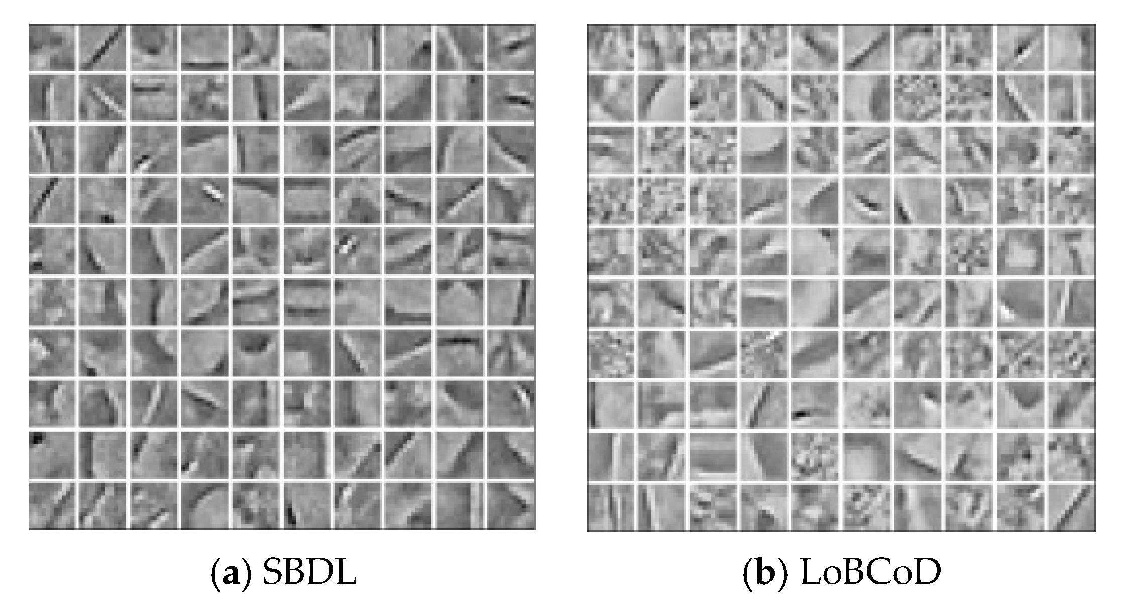
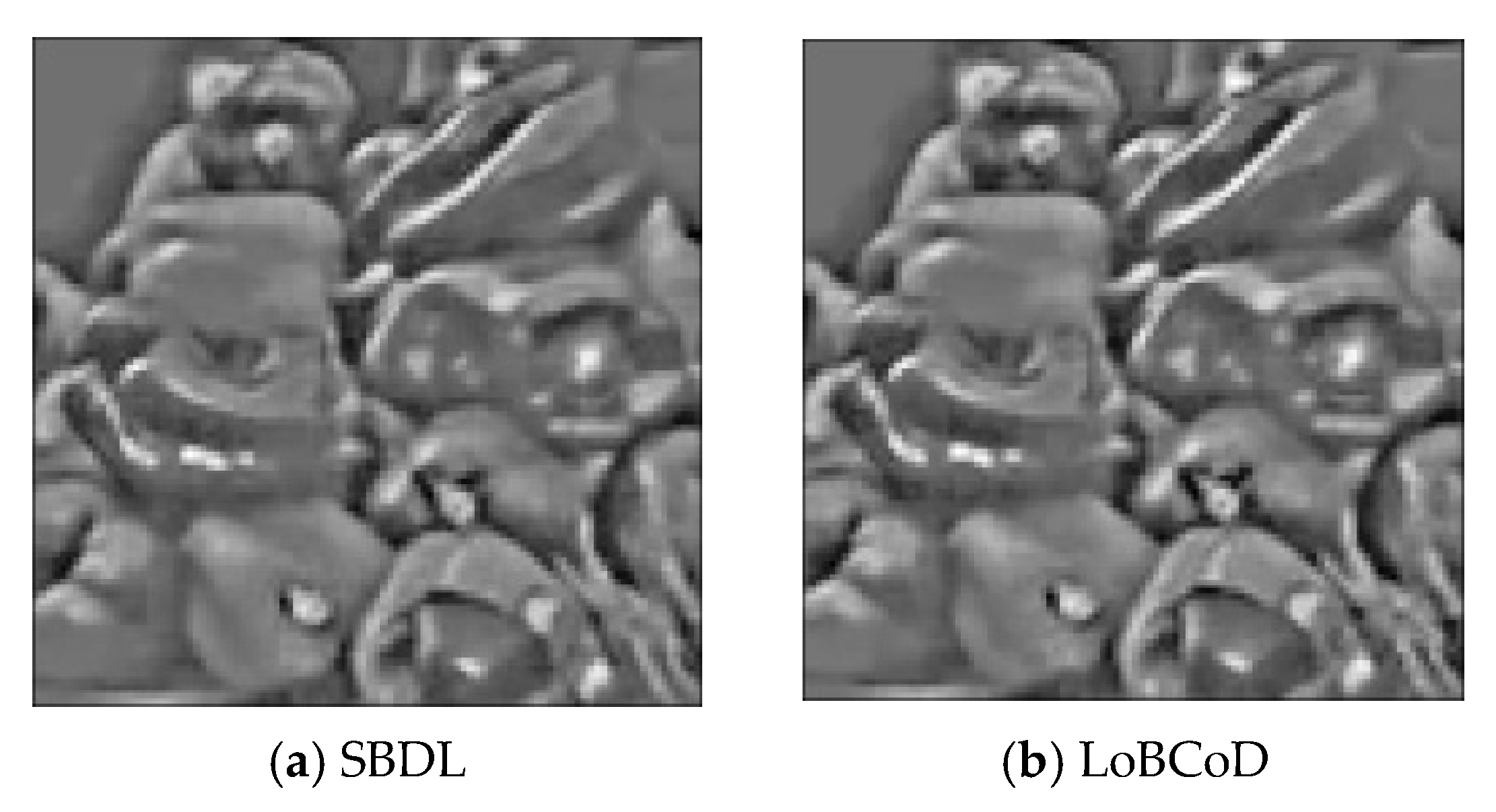
  • SBDL denotes the method proposed in [23] based on convex optimization with an 1 norm-based sparsity-inducing function that uses slices via local processing.
  • Local block coordinate descent (LoBCoD) denotes the method proposed in [24] based on convex optimization with an 1 norm-based sparsity-inducing function that utilizes needle-based representation via local processing.
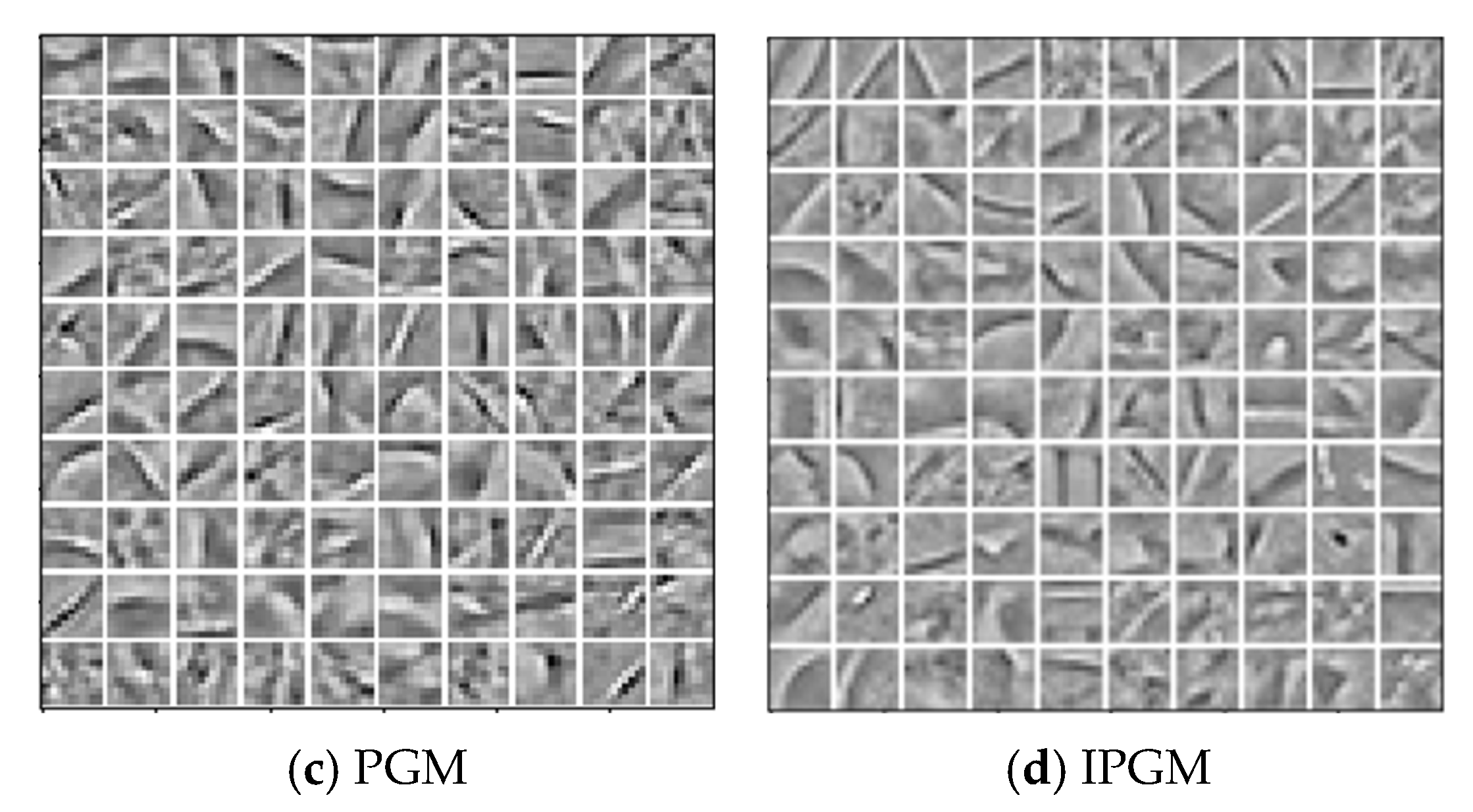
  • The PGM denotes the method proposed in [1] based on convex optimization with an 1 norm-based sparsity-inducing function that uses the Fast Fourier transform (FFT) operation.
  • The IPGM denotes the method proposed in Algorithm 1 in this paper uses needle-based representation via local processing.

7.1.2. Parameter Settings

The parameter settings used for the comparison methods are described as follows:
  • In SBDL [23], the model parameter is λ , and its initial value is 1. The maximum nonzero value of the LARS algorithm is 5. The filter size of the dictionary is 11*11*100. In addition, special techniques are used in the first few iterations of the dictionary learning process.
  • In LoBCoD [24], the model parameter λ is initialized to 1. The maximum nonzero value of the LARS algorithm is 5. The filter format of the dictionary is 11*11*100. In addition, the dictionary learning process first carries out 40 iterations and then uses the proximal gradient descent algorithm.
  • In the PGM [1] model, the Lipschitz constant L is set to 1000 for fruit, and λ = 1 .
  • In the IPGM, the model parameter L t is set at 1000 for fruit, and λ = 1 .

7.1.3. Implementation Details

The computations of the SBDL, LoBCoD, and PGM algorithms, as well as the IPGM algorithm, are performed using a PC with an Intel i5 CPU and 12 GB of memory.

7.2. Efficiency of Dictionary Learning Algorithms

7.2.1. Motivation and Evaluation Metrics
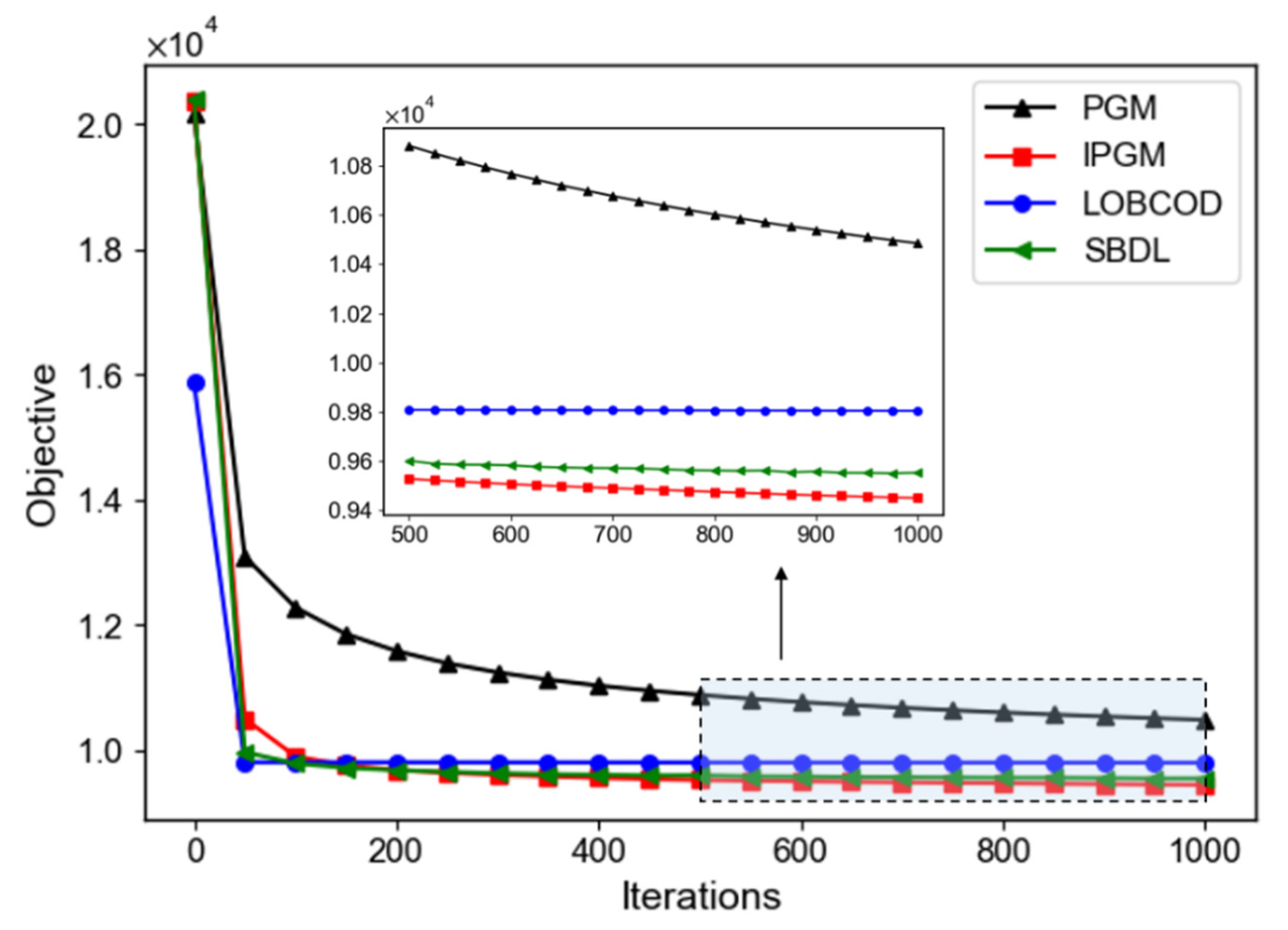
The efficiency and stability of objective function are the most important criteria for evaluating a numerical optimization algorithm. The sequence generated by an efficient dictionary learning algorithm converges quickly to the corresponding clustering point with a lower function value. The relevant evaluation indicators are listed below.
  • Final Value of f + g and the Algorithmic Convergence Properties: In the f + g minimization-based analysis method, we use the function value of the generated sequence to evaluate its optimization efficiency and convergence.
  • Computing Time: We compare the computing times of the SBDL, LoBCoD, PGM, and IPGM algorithms and compare the computing efficiency.

7.2.2. Training Data and Experimental Settings

A set of generic grayscale natural images is used as the training data in this experiment. The set includes 10 fruit images (100 × 100 pixels). It is decomposed into high- and low-frequency components. The means are subtracted. These images are normalized to a range of 0 to 1. The dictionary includes 100 elements, the sizes of which are 11 × 11. One thousand iterations are carried out for each method. The dataset comes from SBDL [23] and LOBCOD [24], and the experimental process refers to the experimental process in references SBDL and LOBCOD. Similar to references [23,24], there is a similar trend in the experimental results under different atomic numbers or different sizes. We give the final objection function value representing the convergence properties and computing time representing convergence efficiency using only the conditions of 100 atoms with a size of 11 × 11 from the fruit grayscale natural images. Each of the average results represents the four trials using different initial dictionaries, from which the initial coefficients were derived.

7.2.3. Results

The experimental results are described as follows. The set of training data described above is used to derive the results. Figure 1 shows the functional values of all compared methods in each iteration of the dictionary learning procedure. In addition, Table 1 shows the experimental data yielded by all compared methods over 1000 iterations. Figure 2 and Figure 3 correspond to the trained dictionaries and reconstructed images of all compared methods after 1000 iterations, respectively.

7.2.4. Discussion

A discussion of the experimental results is as follows. Table 1 shows the experimental results produced by the four algorithms for the fruit dataset, which shows that the IPGM method yields better results in terms of performances. In terms of the objective function values of the four algorithms, the IPGM algorithm is lowest with 9.449 × 10³. In terms of sparsity, except for the poor sparsity of the PGM, there is little difference among the other algorithms. The time consumption of our algorithm is 122.722 s, which is better than that of LoBCoD and the PGM but worse than that of SBDL. The SBDL algorithm calls for the C++ function in the MATLAB program, so it requires less time than the IPGM method. The peak signal-to-noise ratio (PSNR) of the IPGM algorithm is best with 29.438 dB, which is the highest value among the four algorithms. After analyzing Figure 3 above, we see that compared with other algorithms, the IPGM algorithm provides the reconstructed image with the clearest texture details. Generally, the IPGM algorithm has the best performance and the best effect when compared with other algorithms.

7.3. Ablation Experiment

7.3.1. Motivation and Evaluation Metrics

In the proposed IPGM algorithm, the inertia parameters are assigned directly, and they are equivalent to fixed values. Nevertheless, the magnitudes of the inertia parameters have specific impacts on the performance of the algorithm. Therefore, this section uses ablation experiments to analyze the performance of IPGM under different inertia parameters and the performance of IPGM under different optimization conditions.

7.3.2. Training Data and Experimental Settings

The experimental setting of the ablation experiment is consistent with that of the experiment in the previous section. The fruit dataset is also used as the ablation experiment dataset. The dataset comes from SBDL [23] and LOBCOD [24], and the experimental process refers to the experimental process in references SBDL and LOBCOD. We experiment on IPGM algorithms with different inertia parameters under convex optimization constraints and nonconvex optimization constraints.

7.3.3. Results

A discussion of the experimental results is as follows. Table 2 shows the objective function and PSNR values obtained with different inertia parameters under the constraint of nonconvex optimization. Table 3 shows the objective function and PSNR values obtained with different inertia parameters under the constraint of convex optimization.

7.3.4. Discussion

  • The above table summarizes the performance of the IPGM algorithm under different inertia parameter settings. Under nonconvex optimization, with the increase in the inertia parameter, the objective function value decreases, and the PSNR value increases. The effect is the best when the inertia parameter is 0.4. The objective function value is 1.167 × 10⁴, and the PSNR value is 32.734. Under convex optimization, with the increase in the inertia parameter, the value of the objective function decreases, and the value of PSNR increases. The effect is the best when the inertia parameter is 0.9. At this time, the value of the objective function is 9.449 × 10³, and the value of PSNR is 29.438. The results show that the larger the inertia parameter setting is, the better the performance of IPGM is under both convex and nonconvex constraints.
  • According to the ranges of inertia parameters allowed under different constraints, the results in the above table are obtained. By comparing Table 2 and Table 3, it can be found that with the increase in inertia parameters, the PSNR of the IPGM algorithm under convex optimization constraints is higher, the objective function value is low, and the performance improves. Under the constraint of nonconvex optimization, although the PSNR of the IPGM algorithm is high, the value of the objective function is also high, and the performance is not ideal. This result shows that the simple utilized inertia term cannot achieve the perfect effect under the nonconvex constraint. In the future, we will continue to study the IPGM algorithm with dynamic inertia parameters under nonconvex optimization.

8. Conclusions

For the CDL problem, an IPGM algorithm based on a forward–backward splitting algorithm with an inertial term is proposed. The complexity of the algorithm is analyzed, and the convergence of the algorithm is proven. Finally, the IPGM algorithm is compared with other algorithms in terms of performance and effect through experiments. The results show that the IPGM algorithm produces a lower objective function value, lower sparse value, and higher reconstruction PSNR. In summary, the IPGM algorithm has many good theoretical properties, and it is efficient and straightforward.
In addition, according to the allowable range of inertia parameters under different constraints, the ablation experiment of the IPGM algorithm is carried out. According to the experimental results, it can be found that the IPGM algorithm achieves better performance under convex optimization. However, under the nonconvex optimization constraint, the performance of the IPGM algorithm does not reach the ideal value, indicating that the perfect effect cannot be achieved by simply using the inertia term under the nonconvex constraint. In the future, we will further study the IPGM algorithm with dynamic inertia parameters under nonconvex optimization.

Author Contributions

Supervision, Conceptualization, J.L.; Formal analysis, Methodology, Writing, X.W.; Mathematical aspects, F.W.; Review, Funding acquisition, J.W. All authors have read and agreed to the published version of the manuscript.

Funding

This research was funded by Special Projects on Basic Research Cooperation of Beijing, Tianjin and Hebei, grant number 19JCZDJC65600Z, & F2019203583; Central Funds Guiding the Local Science and Technology Development, grant number 206Z5001G; National Natural Science Foundation of China grant number 61473339.

Conflicts of Interest

The authors declare no conflict of interest.

References

  1. Wohlberg, B. Efficient algorithms for convolutional sparse representations. IEEE Trans. Image Process. 2016, 25, 301–315. [Google Scholar] [CrossRef] [PubMed]
  2. Simon, D.; Elad, M. Rethinking the CSC Model for Natural Images. In Proceedings of the Thirty-third Conference on Neural Information Processing Systems (NeurIPS), Vancouver, BC, Canada, 8–14 December 2019; Volume 32, pp. 1–8. [Google Scholar]
  3. Zhang, H.; Patel, V.M. Convolutional Sparse and Low-Rank Coding-Based Image Decomposition. IEEE Trans. Image Process. 2018, 27, 2121–2133. [Google Scholar] [CrossRef] [PubMed]
  4. Yang, L.; Li, C.; Han, J.; Chen, C.; Ye, Q.; Zhang, B.; Cao, X.; Liu, W. Image Reconstruction via Manifold Constrained Convolutional Sparse Coding for Image Sets. IEEE J. Sel. Top. Signal Process. 2017, 11, 1072–1081. [Google Scholar] [CrossRef] [Green Version]
  5. Bao, P.; Sun, H.; Wang, Z.; Zhang, Y.; Xia, W.; Yang, K.; Chen, W.; Chen, M.; Xi, Y.; Niu, S.; et al. Convolutional Sparse Coding for Compressed Sensing CT Reconstruction. IEEE Trans. Med. Imaging 2019, 38, 2607–2619. [Google Scholar] [CrossRef] [PubMed] [Green Version]
  6. Hu, X.-M.; Heide, F.; Dai, Q.; Wetzstein, G. Convolutional Sparse Coding for RGB+NIR Imaging. IEEE Trans. Image Process. 2018, 27, 1611–1625. [Google Scholar] [CrossRef] [PubMed]
  7. Zhu, Y.; Lucey, S. Convolutional Sparse Coding for Trajectory Reconstruction. IEEE Trans. Pattern Anal. Mach. Intell. 2015, 37, 529–540. [Google Scholar] [CrossRef] [Green Version]
  8. Annunziata, R.; Trucco, E. Accelerating Convolutional Sparse Coding for Curvilinear Structures Segmentation by Refining SCIRD-TS Filter Banks. IEEE Trans. Med Imaging 2016, 35, 2381–2392. [Google Scholar] [CrossRef]
  9. Gu, S.; Zuo, W.; Xie, Q.; Meng, D.; Feng, X.; Zhang, L. Convolutional sparse coding for image super-resolution. In Proceedings of the IEEE International Conference on Computer Vision (ICCV), Santiago, Chile, 7–13 December 2015; pp. 1823–1831. [Google Scholar]
  10. Wang, J.; Xia, J.; Yang, Q.; Zhang, Y. Research on Semi-Supervised Sound Event Detection Based on Mean Teacher Models Using ML-LoBCoD-NET. IEEE Access 2020, 8, 38032–38044. [Google Scholar] [CrossRef]
  11. Chen, S.; Billings, S.A.; Luo, W. Orthogonal least squares methods and their application to non-linear system identification. Int. J. Control 1989, 50, 1873–1896. [Google Scholar] [CrossRef]
  12. Chen, S.S.; Donoho, D.L.; Saunders, M.A. Atomic Decomposition by Basis Pursuit. SIAM Rev. 2001, 43, 129–159. [Google Scholar] [CrossRef] [Green Version]
  13. Aharon, M.; Elad, M.; Bruckstein, A. K-svd: An algorithm for designing overcomplete dictionaries for sparse representation. IEEE Trans. Signal Process. 2006, 54, 4311–4322. [Google Scholar] [CrossRef]
  14. Engan, K.; Aase, S.O.; Husoy, J.H. Method of optimal directions for frame design. In Proceedings of the 1999 IEEE International Conference on Acoustics, Speech, and Signal Processing, Phoenix, AZ, USA, 15–19 March 1999; Volume 5, pp. 2443–2446. [Google Scholar]
  15. Mairal, J.; Bach, F.; Ponce, J.; Sapiro, G. Online dictionary learning for sparse coding. In Proceedings of the 26th Annual International Conference on Machine Learning, Montreal, QC, Canada, 14–18 June 2009; pp. 689–696. [Google Scholar]
  16. Sulam, J.; Ophir, B.; Zibulevsky, M.; Elad, M. Trainlets: Dictionary learning in high dimensions. IEEE Trans. Signal Process. 2016, 64, 3180–3193. [Google Scholar] [CrossRef]
  17. Wright, J.; Yang, A.Y.; Ganesh, A.; Sastry, S.S.; Ma, Y. Robust face recognition via sparse representation. IEEE Trans. Pattern Anal. Mach. Intell. 2009, 31, 210–227. [Google Scholar] [CrossRef] [PubMed] [Green Version]
  18. Papyan, V.; Sulam, J.; Elad, M. Working locally thinking globally: Theoretical guarantees for convolutional sparse coding. IEEE Trans. Signal Process. 2017, 65, 5687–5701. [Google Scholar] [CrossRef]
  19. Garcia-Cardona, C.; Wohlberg, B. Convolutional dictionary learning: A comparative review and new algorithms. IEEE Trans. Comput. Imaging 2018, 4, 366–381. [Google Scholar] [CrossRef] [Green Version]
  20. Bristow, H.; Eriksson, A.; Lucey, S. Fast convolutional sparse coding. In Proceedings of the IEEE Conference on Computer Vision and Pattern Recognition (CVPR), Portland, OR, USA, 13–28 June 2013; pp. 391–398. [Google Scholar]
  21. Heide, F.; Heidrich, W.; Wetzstein, G. Fast and flexible convolutional sparse coding. In Proceedings of the IEEE Conference on Computer Vision and Pattern Recognition (CVPR), Boston, MA, USA, 7–12 June 2015; pp. 513–5143. [Google Scholar]
  22. Rey-Otero, I.; Sulam, J.; Elad, M. Variations on the Convolutional Sparse Coding Model. IEEE Trans. Signal Process. 2020, 68, 519–528. [Google Scholar] [CrossRef]
  23. Papyan, V.; Romano, Y.; Sulam, J.; Elad, M. Convolutional dictionary learning via local processing. In Proceedings of the International Conference on Computer Vision (ICCV), Venice, Italy, 22–29 October 2017; pp. 5306–5314. [Google Scholar]
  24. Zisselman, E.; Sulam, J.; Elad, M. A Local Block Coordinate Descent Algorithm for the Convolutional Sparse Coding Model. In Proceedings of the IEEE/CVF Conference on Computer Vision and Pattern Recognition (CVPR), Long Beach, CA, USA, 16–20 June 2019; pp. 8200–8209. [Google Scholar]
  25. Peng, G. Adaptive ADMM for Dictionary Learning in Convolutional Sparse Representation. IEEE Trans. Image Process. 2019, 28, 3408–3422. [Google Scholar] [CrossRef] [PubMed]
  26. Elad, P.; Raja, G. Matching Pursuit Based Convolutional Sparse Coding. In Proceedings of the IEEE International Conference on Acoustics Speech and Signal Processing (ICASSP), Calgary, AB, Canada, 15–20 April 2018; pp. 6847–6851. [Google Scholar]
  27. Chun, I.I.Y.; Fessler, J. Convolutional dictionary learning: Acceleration and convergence. IEEE Trans. Image Process. 2017, 27, 1697–1712. [Google Scholar] [CrossRef] [PubMed]
  28. Peng, G. Joint and Direct Optimization for Dictionary Learning in Convolutional Sparse Representation. IEEE Trans. Neural Netw. Learn. Syst. 2020, 31, 559–573. [Google Scholar] [CrossRef]
  29. Attouch, H.; Bolte, J.; Svaiter, B.F. Convergence of descentmethods for semi-algebraic and tame problems: Proximal algorithms, forward–backward splitting, and regularized Gauss–Seidel methods. Math. Program. 2013, 137, 91–129. [Google Scholar] [CrossRef]
  30. Polyak, B.T. Some methods of speeding up the convergence of iteration methods. USSR Comput. Math. Math. Phys. 1964, 4, 1–17. [Google Scholar] [CrossRef]
  31. Ochs, P.; Chen, Y.; Brox, T.; Pock, T. iPiano: Inertial proximal algorithm for nonconvex optimization. SIAM J. Imaging Sci. 2014, 7, 1388–1419. [Google Scholar] [CrossRef]
  32. Rockafellar, R.T. Monotone Operators and the Proximal Point Algorithm. SIAM J. Appl. Math. 1976, 14, 877–898. [Google Scholar] [CrossRef] [Green Version]
  33. Moursi, W.M. The Forward-Backward Algorithm and the Normal Problem. J. Optim. Theory Appl. 2018, 176, 605–624. [Google Scholar] [CrossRef] [Green Version]
  34. Franci, B.; Staudigl, M.; Grammatico, S. Distributed forward-backward (half) forward algorithms for generalized Nash equilibrium seeking. In Proceedings of the 2020 European Control Conference (ECC), Saint-Petersburg, Russia, 12–15 May 2020; pp. 1274–1279. [Google Scholar]
  35. Molinari, C.; Peypouquet, J.; Roldan, F. Alternating forward–backward splitting for linearly constrained optimization problems. Optim. Lett. 2020, 14, 1071–1088. [Google Scholar] [CrossRef]
  36. Guan, W.B.; Song, W. The forward–backward splitting method and its convergence rate for the minimization of the sum of two functions in Banach spaces. Optim. Lett. 2021, 15, 1735–1758. [Google Scholar] [CrossRef]
  37. Abass, H.A.; Izuchukwu, C.; Mewomo, O.T.; Dong, Q.L. Strong convergence of an inertial forward-backward splitting method for accretive operators in real Hilbert space. Fixed Point Theory 2020, 21, 397–412. [Google Scholar] [CrossRef]
  38. Bot, R.I.; Grad, S.M. Inertial forward–backward methods for solving vector optimization problems. Optimization 2018, 67, 1–16. [Google Scholar] [CrossRef] [PubMed] [Green Version]
  39. Ahookhosh, M.; Hien, L.T.K.; Gillis, N.; Patrinos, P. A block inertial Bregman proximal algorithm for nonsmooth nonconvex problems with application to symmetric nonnegative matrix tri-factorization. J. Optim. Theory Appl. 2020, 190, 234–258. [Google Scholar] [CrossRef]
  40. Xu, J.; Chao, M. An inertial Bregman generalized alternating direction method of multipliers for nonconvex optimization. J. Appl. Math. Comput. 2021, 1–27. [Google Scholar] [CrossRef]
  41. Pock, T.; Sabach, S. Inertial proximal alternating linearized minimization (iPALM) for nonconvex and nonsmooth problems. SIAM J. Imaging Sci. 2016, 9, 1756–1787. [Google Scholar] [CrossRef] [Green Version]
Figure 1. Comparison of the average function values obtained over four trials versus the number of iterations for learning 100 atoms with sizes of 11 × 11 from the grayscale natural fruit images.
Electronics 10 03021 g001
Figure 2. Dictionaries obtained by the four algorithms after 1000 iterations from the grayscale natural fruit images. (ad) is the dictionary obtained by SBDL, LOBCOD, PGM, IPGM, respectively.
Electronics 10 03021 g002aElectronics 10 03021 g002b
Figure 3. Reconstruction images yielded by all compared methods after 1000 iterations from the grayscale natural fruit images. (ad) is the reconstruction images yielded by SBDL, LOBCOD, PGM, IPGM, respectively.
Electronics 10 03021 g003aElectronics 10 03021 g003b
Table 1. The experimental results obtained by all compared methods after 1000 iterations with the grayscale natural fruit images.
FruitSBDLLoBCoDPGMIPGM
Obj9.545 × 1039.857 × 1031.048 × 1049.449 × 103
Data consistent3.067 × 1033.136 × 1033.528 × 103 3.035 × 10³
Regularization6.478 × 1036.722 × 1036.957 × 103 6.415 × 10³
Sparsity0.146%0.141%1.696%0.145%
Time (s)1110.1341879.4001955.3651222.722
PSNR (dB)29.34829.25228.79929.438
Table 2. Objective function values and PSNR values of IPGM models with different inertia parameters under the constraint of nonconvex optimization.
0.10.20.30.4
Obj1.072 × 104 1.059 × 1041.097 × 1041.167 × 104
PSNR31.96032.13932.33532.734
Table 3. Objective function values and PSNR values of IPGM models with different inertia parameters under the constraint of convex optimization.
0.10.20.30.40.50.60.70.80.9
Obj9.737 × 1039.642 × 1039.604 × 1039.569 × 1039.565 × 1039.543 × 1039.516 × 1039.484 × 1039.449 × 103
PSNR29.35029.39429.40129.42729.41429.42229.43329.43129.438
Publisher’s Note: MDPI stays neutral with regard to jurisdictional claims in published maps and institutional affiliations.

