Small-Scale Depthwise Separable Convolutional Neural Networks for Bacteria Classification

Abstract

Bacterial recognition and classification play a vital role in diagnosing disease by determining the presence of large bacteria in the specimens and the symptoms. Artificial intelligence and computer vision widely applied in the medical domain enable improving accuracy and reducing the bacterial recognition and classification time, which aids in making clinical decisions and choosing the proper treatment. This paper aims to provide an approach of 33 bacteria strains’ automated classification from the Digital Images of Bacteria Species (DIBaS) dataset based on small-scale depthwise separable convolutional neural networks. Our five-layer architecture has significant advantages due to the compact model, low computational cost, and reliable recognition accuracy. The experimental results proved that the proposed design reached the highest accuracy of $96.28\%$ with a total of 6600 images and can be executed on limited-resource devices of $3.23$ million parameters and $40.02$ million multiply–accumulate operations (MACs). The number of parameters in this architecture is seven times less than the smallest model listed in the literature.

1. Introduction

Artificial intelligence (AI) has progressed swiftly from object recognition and detection algorithms to software and hardware’s incredible execution capabilities in recent decades. Image and video classification [1,2,3], natural language processing [4], robotics [5], and health-care [6,7] are just a few of the fields where AI-based solutions have surpassed human accuracy and insights. Applying AI and computer vision to biomedical sciences has opened up immense potential for exploring different areas and improving existing medical technology, particularly bacterial recognition. These methods automatically enhance the detection and classification of bacteria species, are highly accurate, reduce cost and time, and avoid researchers’ risk of infection.

Deep-learning approaches, especially deep convolutional neural networks (DCNNs), are currently some of the most notable machine-learning algorithms for dealing with complex tasks that only experienced experts could address in the past. In computer vision or image classification applications, DCNNs may obtain higher accuracy and even exceed non-learning algorithms. The higher accuracy of DCNNs comes from extracting automated high-level features after using statistical learning from a large amount of input training data. Statistical learning supports representing the input space efficiently and well-generalized. However, this capability also requires high computational effort, as well as large memory sizes. When the network size grows exponentially, the respective computational effort and memory size also rise. Due to the personal characteristics of power supply and dimension, these networks are hard to execute on the limited hardware resources of medical devices. Therefore, structural model size reduction [8] and parameter optimization [9,10] are offered to maintain the inference performance of deep neural networks.

Early detection and identification of pathogenic bacteria in food, water, and bodily fluids are essential, yet challenging, owing to sample complexities and large sample volumes that need to be rapidly screened. Existing screening methods based on plate counting or molecular analysis present some tradeoffs regarding detection time, accuracy/sensitivity, cost, and sample preparation complexity. The standard procedure in bacterial detection begins with the collection of various types of test materials. Next, the clinical materials are directly handled on special media (Gram stain, cultivated on medium agar) for 5–20 min. The material incubates under specific temperature conditions: 37 °C, 5–7% CO₂ (usually taking 18–24 h). The initial identification of bacteria depends on the assessment of the cell shapes observed under the microscope and the growth rate, type, shape, color, and smell of the colonies (several minutes to 18–24 h). Such analysis allows the assignment to a bacteria type; however, identifying the species is usually impossible due to their significant similarity. Because of that, further analysis consisting of biochemical tests is necessary (16–24 h). As a result, from culture to species identification, the entire diagnostic process can last 2–3 d.

This paper presents a convolutional-neural-network-based approach for the reliably accurate recognition of bacterial species in high-resolution microscopy images for rapidly detecting and classifying related species. The proposed method consists of two crucial stages. Firstly, data augmentation techniques are applied to create a new dataset of species derived from the DIBaS dataset to sufficiently take advantage of the fine features from a large number of bacteria images and to avoid the overfitting issue. Secondly, a small-scale depthwise separable CNN architecture (DS-CNN) for bacteria recognition is built. With three main convolutional layers and an efficient classifier, this model aims to recognize bacteria in the images. The recommended detection and classification method was tested using the partial DIBaS dataset, with 33 various classes of bacteria, and gained a bacterial strain classification rate of $96.28\%$. The obtained results still ensure the superiority of the stated method over the state-of-the-art CNN model, but at the same time, fit with low-energy, low-resource devices. More specifically, our design uses only about three million parameters (equivalent to small memory size utilization), about seven-times less than the most efficient model in related papers, and the computational complexity expressed via the MAC operations is forty million. We emphasize the tradeoff between the model’s accuracy reduction (2–3%) and the resource usage of the lowest memory and computation complexity.

This paper has the following main contributions:

• The DS-CNN was exploited to construct a compact network architecture for the automated recognition and classification of 33 bacteria species in the DIBaS dataset with reliable accuracy and less time consumption;
• As part of our methodology, we incorporated preprocessing and data augmentation strategies to improve the model’s input quality and achieve higher classification accuracy.

We organized the rest of this paper as follows: In Section 2, you will find a few related articles for the bacterial classification task on the DIBaS dataset using convolutional neural networks. Section 3 briefly introduces C-Conv and DS-Conv, as well as the proposed architectural structure. The content of Section 4 gives the materials and methods that we offer in this study. Setups for the experimentation are discussed in Section 5. Section 6 gives the results of classifying 33 types of bacteria and discusses them. In Section 7, a conclusion and recommendations for further work are offered.

2. Related Works

Colony morphology, biochemical properties, and molecular phylogenetic approaches are all used to identify bacteria [11]. Microbiologists prefer the reading of bacteria in digital microscopic images by colony morphology, which is more accurate than molecular phylogenetics [12]. Each type of bacteria has distinct structural and geometric characteristics that describe its size, shape [13], color [14], texture, height, and edge [15,16]. These characteristics may help distinguish bacteria species, observe bacteria growth, observe microbial interactions, and aid in drug discovery and disease diagnosis.

Generally, traditional laboratory methods for analyzing microbiological images sometimes reveal incorrect bacteria recognition, which requires unique experience and a longer execution time. In recent years, the combination of image-processing techniques with ML and DL algorithms has become popular to help detect and classify bacteria images, achieving outstanding results. Image processing currently acts as the data preprocessing stage to make bacterial classification models more efficient. Therefore, the automatic classification techniques [17] of bacterial samples are more valuable than traditional visual observations by biologists due to the accurate classifier, low cost, and rapid diagnosis.

Without labels, Raman optical spectroscopy could detect, identify, and test bacteria for antibiotic susceptibility. However, the weak Raman signals produced by bacterial cells and the diversity of bacterial species and phenotypes continue to pose a clinical challenge. Ho et al. [18] collected Raman spectra from bacteria and used deep learning to identify 30 common bacterial pathogens. The average accuracy for antibiotic treatment identification was $97.0\pm 0.3\%$ even with low signal-to-noise spectra. The authors showed that this method accurately distinguishes MRSA and MSSA isolates. Their findings were tested on 50 clinical isolates. The experiment only utilized ten bacterial spectra from each patient isolate to identify 99.7% of treatments. The method can be used for culture-free pathogen detection and antibiotic susceptibility testing in blood, urine, and sputum.

Kang et al. [19] designed a set of advanced deep-learning frameworks, including the long short-term memory (LSTM) network, the deep residual network (ResNet), and the one-dimensional convolutional neural network (1D-CNN), for the classification of foodborne bacteria using hyperspectral microscopic imaging (HMI) technology. Five popular foodborne bacterial cultures ($Campylobacter jejuni$, $generic E. coli$, $Listeria innocua$, $Staphylococcus aureus$, and $Salmonella typhimurium$) were collected by the U.S. Department of Agriculture’s Poultry Microbiological Safety and Processing Research Unit (PMSPRU) in Athens, Georgia. During the experiment, the given dataset contained 5000 images that were randomly partitioned into 72% (3600 cells), 18 % (900 cells), and 10% (500 cells) for training, validation, and testing, respectively. According to the experimental results, LSTM, ResNet, and 1D-CNN achieved an accuracy of 92.2%, 93.8%, and 96.2%, respectively.

Sajedi et al. [20] employed the extreme gradient boosting classification (XGBoost) approach combined with a set of common image-processing methods to classify three different Myxobacterial suborders, i.e., Cystobacterineae, Sorangiineae, and Nannocystineae. The proposed method consisted of two processes: firstly, using the Gabor transform to extract texture features and then applying XGBoost to recognize three categories of bacteria. The accuracy obtained by the suggested model was 90.28%. In addition, the authors also wrote some literature reviews related to the classification of bacteria by using ML algorithms, including deep neural networks.

Tamiev et al. [21] investigated the possibility of using classification-type convolutional neural networks (cCNNs) to classify bacteria subpopulations (in this case, biofilm stages) from fluorescent microscope images. Annotated training datasets including null bumper (NB), blended bumper (BB), and advanced rotation (AR) after the image-processing workflow were used to test the classification performance of the cCNN (AR). When trained on a small dataset (81 images), advanced rotation improved the CNN’s accuracy and confidence for smaller clusters (debris artifacts, single, double, and triple cells) with an 86% accuracy. Larger clusters (4–10 cell clusters) would require more training data to the improve accuracy (50–66%). While individual classification accuracy was lower than desired when the total number of cells was added up, these inconsistencies balanced out, and their proposed algorithm performed nearly as well as manual counting over 24 images. Compared to multiple manual counts, this AR-trained cCNN algorithm reduced interoperator variability by $10.2\times$ and increased processing speed by $3.8\times$.

Mhathesh et al. [22] classified 3D light-sheet fluorescence microscopy images of larval zebrafish using the DL technique in 2020. The authors applied a CNN for the classification of bacterial images. That study utilized various activation functions, i.e., sigmoid, Tanh, and ReLU, to analyze the model’s accuracy. The authors then compared the given results with other classifiers such as the support vector classifier, random forest, and ConvNet. The presented method achieved an accuracy of 95%, which outperformed the other selected techniques.

In addition, another approach to bacteria detection is to use microelectronic sensors. Korzeniewska et al. [23] presented the interaction between silver and Staphylococcus aureus as being used to detect the presence and measure the numbers of bacteria. The increase in the number of bacteria caused changes in the electrical parameters of the sensor. The most extensive changes in electrical parameters were observed at 100 Hz and 120 Hz and within the 28–69 h time window from initial bacterial infection. The results from this work can be implemented in various domains, such as biomedical or industrial products.

So far, the deep-learning approach in the analysis of microbiological images (on the same full DIBaS dataset), taking into account microbial detection and classification, has been investigated and undertaken in several related papers.

Zielinski et al. [24] publicly, for the first time, offered the DIBaS dataset collected by the Chair of Microbiology at Jagiellonian University in Krakow, Poland. The DIBaS is utilized as standard data for biomedical researchers to classify bacteria strains and compare their solutions. The authors applied the Fisher vector (FV), local image descriptors, and the pooling encoder to obtain the image descriptors of the DIBaS bacterial image dataset. In addition, two machine-learning algorithms, the support vector machine (SVM) and random forest (RF) techniques, combined with convolutional neural network (CNN) models such as AlexNet, VGG-M, and VGG-VD were employed to group bacterial microorganisms into 33 classes. The classification accuracy in this article was 97.24 ± 1.07%.

When Nasip and his colleagues [25] used the DIBaS dataset to pretrain deep CNN architectures based on the VGGNet and AlexNet models, they could classify 33 different types of bacteria. Images of these species with an original resolution of $2048\times 1532$ pixels were divided into $227\times 227$ (AlexNet input size) and $224\times 224$ (VGGNet input size) images to fit with the model inputs. Following this way, in total, the new dataset had 35,600 images overall. Then, $80\%$ (28,512) of the images were utilized for training and the remaining $20\%$ (7128) for testing. The classification accuracy of VGGNet and AlexNet was 98.25% and 97.53%, respectively. It could be concluded that the success rate would vary depending on the training model exploited and the data’s number and size.

M. Talo’s research [26] described an automated deep-learning-based classification approach to classify bacterial images into 33 categories. The ResNet-50 CNN structure was pretrained with the full DIBaS dataset, and a transfer learning technique [27] was employed to pace up the training steps and enhance the network’s overall classification performance. The model was trained for 50 epochs in about 31 min and 48 s and tested on an Ubuntu 16.04 server using an NVIDIA GeForce GTX 1080 TI graphic card. A five-fold cross-validation technique that evaluated the model’s performance was used. The experiments were repeated five times, and the average of five trials on the validation sets was given as the classification performance for the overall model. His suggestion accomplished a perfect classification accuracy of $99.2\%$.

Khalifa et al. [28] aimed to present a deep neural network architecture based on the AlexNet model to determine the bacterial colony classification problem. Additionally, a strategy for training and testing was introduced that heavily relies on data augmentation methods. The dataset used was limited in size, containing 660 images representing 33 distinct classes of a bacterial colony. Any neural network could hardly learn directly from this small amount of data; hence, the neural network could meet overfitting or underfitting issues when training. The training and testing strategy implemented resulted in a noticeable improvement in the training and testing phases. It increased the number of images in the dataset to 6600 for the training phase and 5940 for the verification phase. When combined with the augmentation techniques, the proposed neural network achieved a testing accuracy of 98.22%.

Anna Plichta proposed two different solutions for automatically recognizing 20 species and genera of bacteria in the DIBaS database. The classification was made based on the analysis of seven physical characteristics of bacterial cells by means of the product of the weights of classifiers [29] and a decision tree algorithm [30]. The same images and the same set of seven implemented classifiers were used to classify the samples and recognize the analyzed species and genera of bacteria in both methods. The proposed decision tree tended to use highly correct classifiers, such as the bacterial cell color, which has the highest correctness of all and can obtain the best possible results if using the boosted decision tree method. The accuracy (correctness) of this decision tree amounted to 83.77%, although changes in the decision tree remained at 95.94%. At the same time, classification through the method based on the product of the weights of the classifiers brought better results. For all the analyzed species and genera of bacteria, correct classification by this product of weights method amounted to 90.45%, and its sensitivity was 100%.

Sanskruti Patel [31] created a transfer-learning-based modified CNN model for bacterial colony classification. This method made use of a VGG-16 model that had been previously trained, with the last block being replaced by atrous convolution with a dilation rate of two. The model was implemented on a DIBaS dataset of a bacterial colony, containing 660 images and 33 classification classes. As a result, the suggested architecture significantly improved the accuracy, reaching $95.06\%$ training accuracy, $93.38\%$ validation accuracy, and $94.85\%$ test accuracy. If using more bacterial colony images, a higher achievement of the architecture could be obtained. In the future, it might be possible to develop an automated embedded device for in-field bacterial colony classification similar to what is currently available.

To save time in the training process, as well as improve the accuracy of the models that were applied in several related works, all authors exploited a method called transfer learning by using weight files pretrained from the ImageNet dataset and adjusting the model outputs according to their goals. However, one of the most significant barriers to transfer learning is currently the problem of negative transfer. Transfer learning only operates correctly if the initial and target issues are similar enough for the first round of training to be relevant. If the first training cycle is too far off the mark, the model may perform worse than if it had never been trained. Right now, there are no clear benchmarks for determining which types of training are sufficiently related or how this should be measured. A training process from scratch is chosen to avoid this challenge and ensure the model’s reliability.

In addition, the major problem is that CNNs include so many parameters (especially weights) that resource-constrained embedded hardware cannot store them in on-chip memory. However, accessing the off-chip memory leads to a negative impact on performance. Another option is to employ high-bandwidth off-chip DRAM, which is found in a graphics processing units (GPUs). However, this causes considerable power dissipation and hardly meets the low power consumption requirements. Hence, the DS-Conv block is suggested for a small-scale CNN model construction to satisfy the needs of power consumption and resources.

3. Overview of the Depthwise Separable Convolutional Neural Network

This section provides the fundamental structures of the standard convolutional block (C-Conv) and the depthwise separable convolutional block (DS-Conv). We then analyze these two main blocks’ computational complexity to demonstrate that DS-Conv has more computational cost efficiency.

3.1. DS-CNN Layer Primer

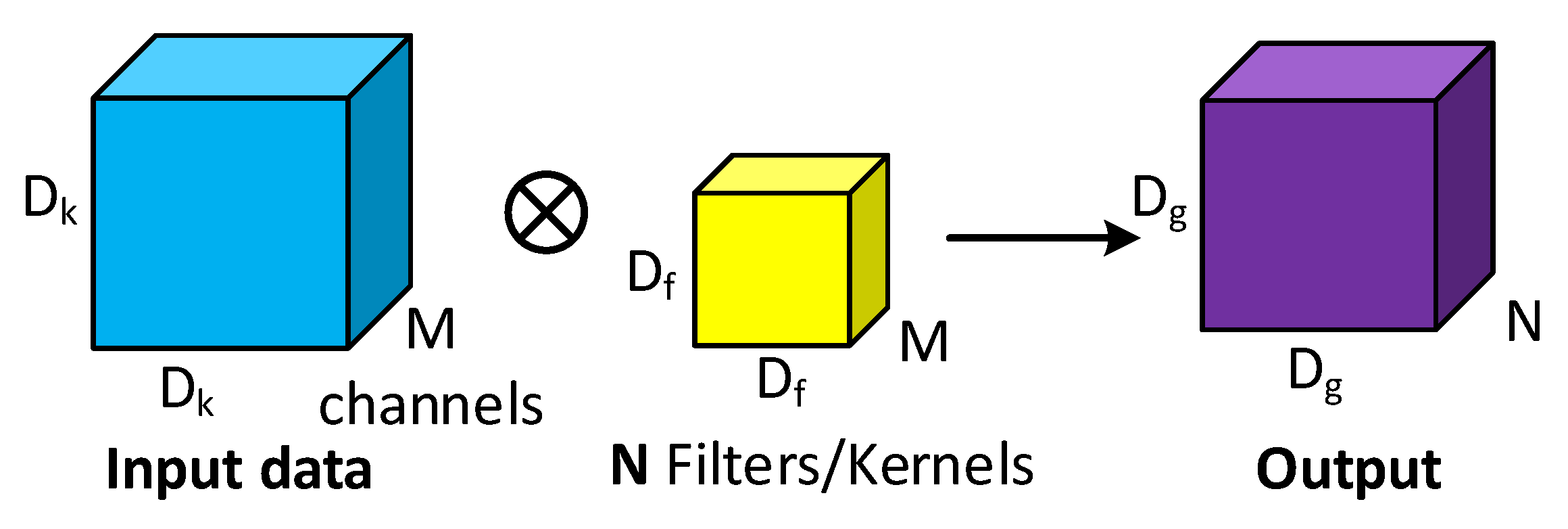
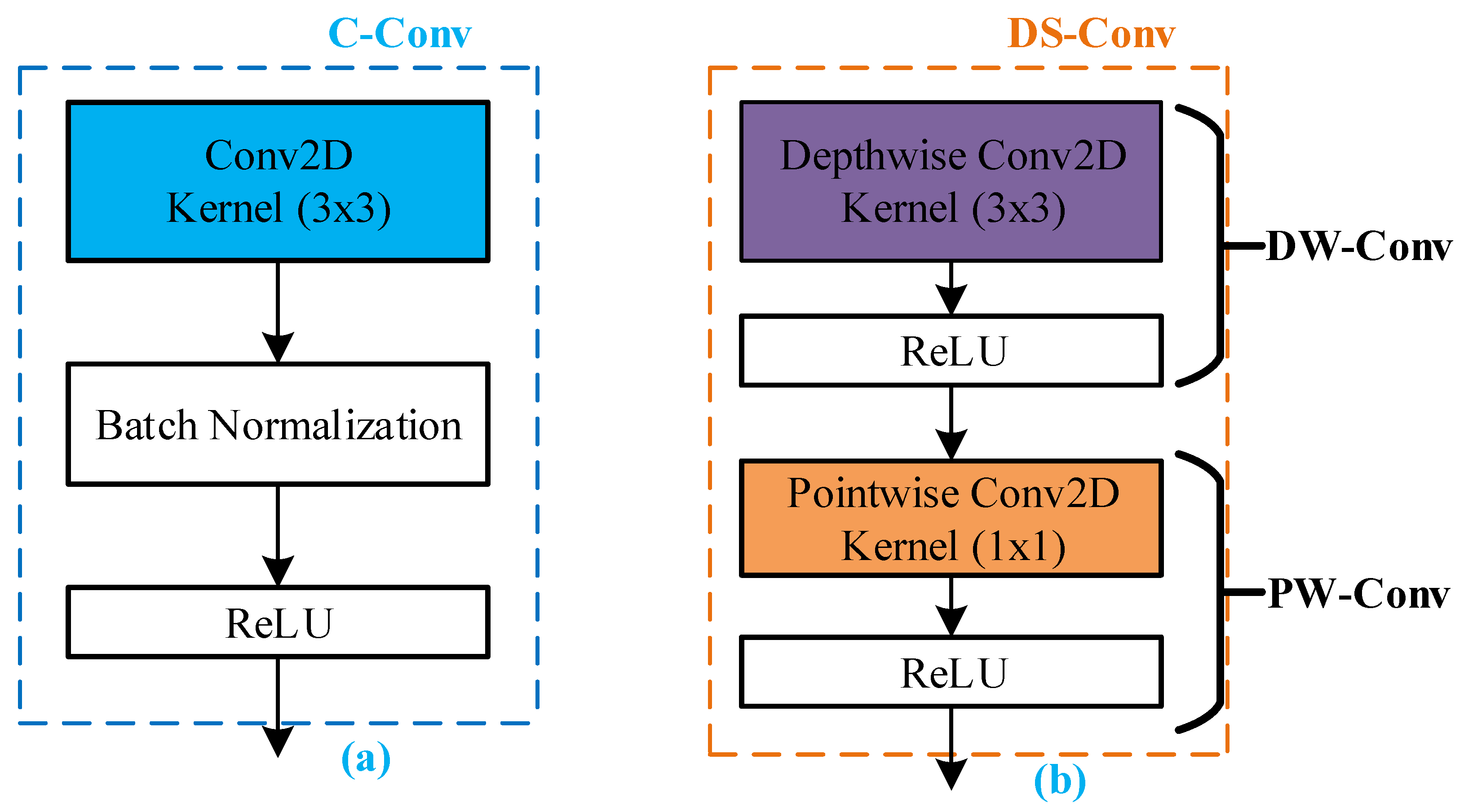
3.1.1. Conventional Convolution Block

LeCun et al. [32] published the first version of CNN in 1998, and it has been firmly applied to address computer vision (CV) tasks such as image classification, speech recognition, face recognition, and natural language processing. In general, two significant features contributed to the CNN’s success. Firstly, it enhances the recognition rate for its receptive field, similar to human visual cells. Secondly, local connection and weight sharing also significantly reduce the number of network parameters and alleviate overfitting compared with a fully connected deep neural network. In this paper, we refer to the CNN as mentioned above as conventional CNN (C-Conv).

As for conventional convolutions, as shown in Figure 1, each input channel requires a convolution operation such that the number of convolution kernels is the same as the output channel. The result of each output channel is the sum of its corresponding convolution kernels and the convolutional results of all input channels. Assume that the dimension of the input feature is $D_k\times D_k\times M$, where $D_k$, $D_k$, and M are the width, height, and the number of input channels, respectively. Each convolutional layer uses filters of size $D_f\times D_f$ (one channel per filter) with N filters.

Figure 1. The operation of a conventional convolution.

The common sizes of filters in CNNs are $11\times 11$, $5\times 5$, and $3\times 3$. The output is $D_g\times D_g\times N$, where $D_g$, $D_g$, and N are the width, height, and the number of output channels, respectively. Let the total number of trainable parameters in conventional convolution be $P_{C-Conv}$ (without considering bias) and the number of floating-point calculations be $C_{C-Conv}$ in a standard convolution process. They may be computed as shown in Equations (1) and (2) below:

$$P_{C-Conv}=D_f^2\times M\times N$$

(1)

$$C_{C-Conv}=D_f^2\times M\times D_g^2\times N$$

(2)

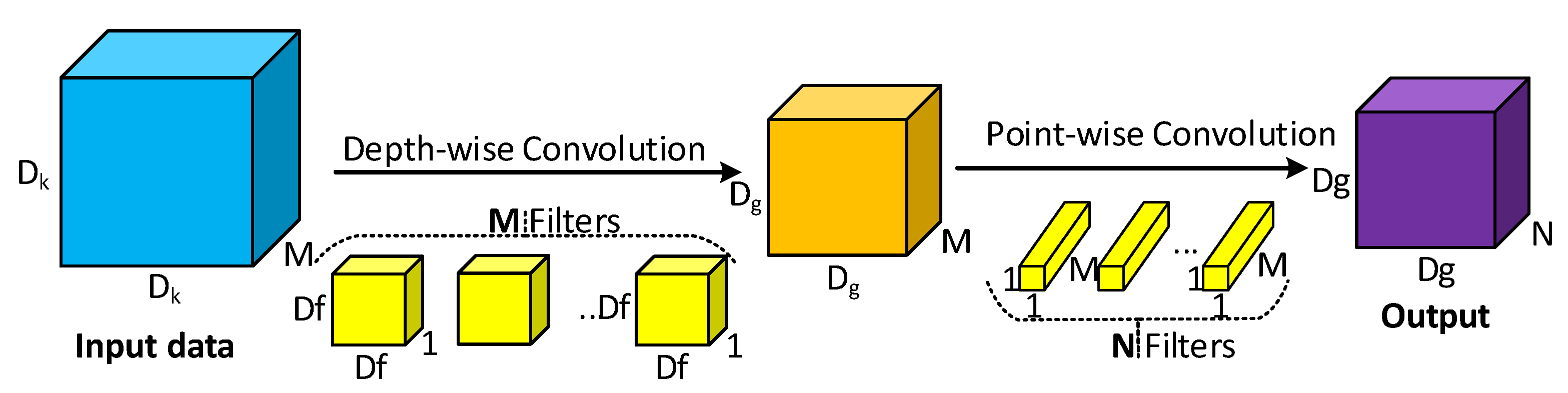
3.1.2. Depthwise Separable Convolution

Depthwise separable convolution first appeared in L. Sifre’s [33] thesis in 2014 and was applied in MobileNet [34] and the Xception model [35] to replace conventional convolutional layers. DS-Conv is a factorized form of standard spatial convolution. It is composed of depthwise convolution and 1 × 1 convolution (also known as pointwise convolution). The traditional spatial convolution algorithm primarily extracts channelwise features and then combines them to generate new representations. Separately, depthwise and pointwise convolutions can be used to accomplish such two-step tasks.

This is depicted in Figure 2, in which the size of the input image is $D_k\times D_k\times M$, where $D_k$ is the height and width of the input image, M is the number of input channels. Each convolutional layer uses filters of size $D_f\times D_f\times 1$ with M filters. When M filters are taken to slide through the input image, one intermediate feature map $D_g\times D_g\times M$ is produced by convolving each input feature map with a 2D filter kernel in the depthwise convolution block. It is applied as the input of the next convolution. For the pointwise convolution, the convolution kernels size is 1 × 1; the number of channels on each convolution kernel must be the same as the number of input feature map channels. Let the number of the convolution kernels be N, and then, the output feature map would become $D_g\times D_g\times N$ after convolution.

Figure 2. Structure of the depthwise separable convolution block.

As illustrated in Figure 2 with a process of depthwise separable convolution, the parameter $P_{DS-Conv}$ and the floating-point calculation cost $C_{DS-Conv}$ are the sums of the depthwise and $1\times 1$ pointwise convolutions. Hence, $P_{DS-Conv}$ and $C_{DS-Conv}$ are calculated as shown in Equations (3) and (4), respectively:

$$P_{DS-Conv}=D_f^2\times M+M\times N$$

(3)

$$C_{DS-Conv}=D_f^2\times 1\times D_g^2\times M+1^2\times M\times D_g^2\times N=(D_f^2+N)\times D_g^2\times M$$

(4)

Therefore, the ratio of parameters $r1$ of Equations (1) and (3), the ratio of computation cost $r2$ of Equations (2) and (4) between depthwise separable convolution and the normal convolution can be written as:

$$r1=\frac{P_{DS-Conv}}{P_{C-Conv}}=\frac{D_f^2\times M+M\times N}{D_f^2\times M\times N}=\frac{1}{N}+\frac{1}{{D_f}^2}\ll 1$$

(5)

$$r2=\frac{C_{DS-Conv}}{C_{C-Conv}}=\frac{(D_f^2+N)\times D_g^2\times M}{D_f^2\times N\times D_g^2\times M}=\frac{1}{N}+\frac{1}{{D_f}^2}\ll 1$$

(6)

due to $N\gg 1$ and $D_g^2>1$.

It can be clearly seen that the parameters and computational cost are reduced to $\frac{1}{N}+\frac{1}{{D_f}^2}$ compared to the conventional convolution operation. Our study employed a $D_f\times D_f=3\times 3$ depthwise convolution filter size and the number of filters ($N=64$), so the computation complexity and number of parameters of DS-Conv in each neuron are ∼13-times less than the same neuron in conventional convolution and only tradeoff a slight accuracy loss for the overall architecture. Further, DS-Conv essentially converts continuous multiplication into continuous addition, so the network’s redundancy becomes reduced. As a result, the computational efficiency of the network is greatly improved.

3.1.3. Activation Functions

A differentiable and nonlinear function is applied to the feature map, and then, the result is sent to the subsequence layer as the input. The function is called the activation function. Activation provides nonlinearity to the network and aids high-order polynomials’ learning so that the network can learn and perform a more complex task. There are various types of activation functions, and the most popular kinds that are commonly utilized are sigmoid and rectified linear units (ReLUs):

• Sigmoid function:

  $$Sigmoid\left(x\right)=\frac{e^x}{1+e^x}$$

  (7)

The sigmoid function is one of the most typical nonlinear activation function with an overall S-shape. The sigmoid function that maps a real number to $[0,1]$ is often used for binary classification. Besides advantages such as gradient smoothing and precise predictions, there are some main drawbacks, including the fact that the sigmoid outputs are not zero-centered, the vanishing gradient problem, where weights in lower layers are virtually unchanged, and the high-cost computation;

• Rectified linear unit (ReLU):

  $$ReLU\left(x\right)=\left\{\begin{array}{c}xx>0\hfill \\ 0x\le 0\hfill \end{array}\right.$$

  (8)

  where x is the input to the neuron.

The ReLU layer is a nonlinear operation that is performed after every convolutional layer. Its output is given by $max(0,x)$. The purpose of ReLU is to introduce nonlinearity in the CNN after the linear operation of convolution since the network needs to learn from real-world data, which are nonlinear, and for the network to generalize or adapt with a variety of data. Compared to sigmoid functions, rectified linear units support faster and more effective training of deep neural architectures and complex datasets. ReLU has several benefits: the number of active neurons is reduced due to a zero in the negative domain and not saturated; it is highly computationally efficient; it speeds up learning; it prevents the vanishing gradient problem.

3.1.4. Batch Normalization

Controlling the input distribution across layers can speed up the training process and improve the accuracy significantly. Accordingly, the distribution of the layer input activation $\left(\sigma ,\mu \right)$ is normalized such that it has a zero mean and a unit standard deviation. As visualized in Equation (9), in batch normalization (BN), the normalized value is further scaled and shifted, where the parameters ($\gamma$, $\beta$) are learned from the training process [36]. $\epsilon$ is a small constant to avoid numerical problems. BN is mainly performed between the CONV or FC layer and the nonlinear function.

$$y=\frac{x-u}{\sqrt{{\sigma }^2+\epsilon }}\gamma +\beta$$

(9)

3.1.5. Pooling Layer

A key aspect of convolutional neural networks is the pooling layer, typically applied after the convolutional layers. Pooling layers (also called subsampling or downsampling) reduce each feature map’s dimensionality, but retain the essential information. For the group of neurons in each receptive field, they return a single value that contains a statistic about the group, e.g., the maximum or the average value. The well-known methods for pooling execution consist of three different types: max, average, and sum. In practice, max pooling has been widely utilized and works better.

3.1.6. Fully Connected Layer

The convolution/pooling process’s output is flattened and transformed into a single vector of values. Each value represents the probability that the features and labels are related. By utilizing the features derived from the process of the previous layer, the fully connected (FC) layer is employed to convert the images to labels. Each neuron prioritizes the tag that corresponds to the received weight. Following that, all neurons will vote on which class should win the classification.

3.1.7. Dropout

Multiple hidden layers are used to learn more complex features, followed by FC layers for decision-making. FC layers are those that are connected to all features and are prone to overfitting. Over-fitting is a problem that occurs when a model is trained and performs so well on the training data that it has a detrimental effect on the model’s performance on new data. The insertion of a dropout layer [37] into the model, where some neurons and their connections are randomly removed from the network during training, helps avoid this problem significantly. The network size becomes smaller, and any incoming or outgoing connections to the dropped out node are also terminated.

To avoid overfitting during training, one dropout layer was added to the proposed network. The dropout rate was set at $0.25$ and $0.5$.

3.1.8. Classifier Layers

In the last layer, we used the softmax activation function, a popular selection for the final layer in most state-of-the-art deep-learning architectures, to normalize the output of a probability distribution over predicted output classes that sum to one. This function is a generalization of the logistic function to multiple dimensions, and its role is to normalize the output between zero and one. It is frequently employed in both binary and multi-class tasks, provided that each object belongs to one class. The following Equation (10) computes the softmax function:

$$Softmax\left(x_i\right)=\frac{e^{x_i}}{{\sum }_{j=0}^N{e}^{x_j}}\left(i=1,2,\dots ,N\right)$$

(10)

where $x_i$ are the elements of the input vector to the softmax function, $e^{x_i}$ is the standard exponential function applied to each element of the input vector, and ${\sum }_{j=0}^N{e}^{x_j}$ is the normalization term, which ensures that all the output values of the function will sum to one and each will be in the range (0, 1).

We designed a dedicated classifier at the end of the final layer. This classifier consists of 1 FC layer, 1 dropout layer with a rate of 0.25 (which randomly cuts off some connections to reduce the overfitting problem), and 1 Softmax layer for the image classification tasks.

3.1.9. Learning Rate and Optimizers

The learning rate is an essential component for training a CNN. The learning rate is the step size taken into account during training, which speeds up the process. However, choosing the appropriate value for the learning rate is important. If choosing $\eta$ with a high value, the network may start diverging instead of converging. On the other hand, selecting a smaller value for $\eta$ will result in more time for the network to converge. In addition, it may quickly become stuck in local minima. The popular solution that addresses this problem is to reduce the learning rate during training. In this article, we set the learning rate to $\eta =1$ × ${10}^{-4}$.

In convolutional neural networks, non-convex functions often need to be optimized. Mathematical methods require massive computing power, so optimizers are utilized in the training process to minimize the loss function for acquiring optimal network parameters within an acceptable time. Standard optimization algorithms including RMSprop, Adam, Adamax, and Nadam were employed for our model. RMSprop considers only the magnitude of the gradient of the immediately previous iteration. The Adam optimization approach is suggested based on the momentum and the magnitude of the gradient for calculating the adaptive learning rate similar to RMSprop. Adam has improved overall accuracy and helps with efficient training with the better convergence of deep-learning algorithms. These solutions provide some advantages, as well as existing drawbacks, so that each optimizer was verified for the scenarios in the experiment.

3.2. The Proposed Architecture

The proposed block diagram in the bacteria classification process is described in Figure 3. Our architecture consists of four main blocks, from input microscopy images to the classification process, in which the second and third blocks are the main contributions. The data preprocessing block enhances the size and quality of data, as well as resolves imbalances in the dataset and overfitting issues. This block is composed of three stages. Firstly, the input images to be detected were resized from the original dimensions to $224\times 224$, and the number of channels was set at three to fit with the expected input of the model. Then, data augmentation was applied by using transformation to artificially increase the number of images for the training process. Last, the new datasets were split into three sets: training, validation, and testing, with percentages of $70/20/10$, respectively.

Figure 3. Schematic overview of the network architecture.

The schematic overview of the proposed model is intelligibly depicted with five crucial layers, in which the first three convolutional layers extract image features with a depth of sixty-four and filter sizes of 3 × 3 and $1\times 1$. After that, one FC layer and one softmax function are used for data flattening and bacteria species classification, respectively. In addition, we inserted BN and dropout layers to normalize the data and avoid overfitting during training.

Figure 4a,b illustrates the internal structure of C-Conv and DS-Conv in detail, respectively. From Figure 4a, C-Conv only carries out a Conv2D operation, then passes through the BN layer, and finally enters into the activation function ReLU layer to obtain the output of C-Conv. Similarly, in Figure 4b, DS-Conv carries out the DW-Conv operation first, then penetrates the ReLU layer to obtain the output of DW-Conv. After that, the output of the DW-Conv layer is input into the PW-Conv layer. PW-Conv performs a pointwise convolution operation with a $1\times 1$ filter size, then passes through the activation function ReLU layer to obtain the output of PW-Conv. The output of PW-Conv is that of DS-Conv. Here, BN after C-Conv helps accelerate deep network training by reducing the internal covariate shift [36], normalizing the input data x to $[0,1]$, and conforming to the standard normal distribution. In addition, ReLU was utilized as an activation function.

Figure 4. Internal structure. (a) C-Conv ; (b) DS-Conv.

Table 1 represents a small-scale CNN architecture based on depthwise separable convolution (DS-Conv) with its detailed specification. Following the conventional convolutional layer (C-Conv), the BN layer, and the max pooling layer, the depthwise convolution (DW-Conv), pointwise convolution (PW-Conv), and max pooling ($Max\_pool$) layers are added. After two consecutive depthwise separable and max pooling layers, there are FC layers and the softmax classifier to classify 33 outputs. We also calculated the trainable parameters (weight and bias) and the computation cost (multiply–accumulate operations (MACs)) of the design.

Table 1. The proposed architecture specification.

Layer	Type	Filter Size	Output Shape	Parameters (M)	MACs (M)
Input			224 × 224 × 3
Conv1	Conv_1/Stride 2	3 × 3 × 3 × 64	112 × 112 × 64	0.002	21.68
	Batch Norm	-	112 × 112 × 64	0.0003	0
	Max-Pooling_1	Pool 2 × 2	56 × 56 × 64	0	0
Conv2	DW-Conv_2	3 × 3 × 1 × 64	56 × 56 × 64	0.0006	1.80
	PW-Conv_2	1 × 1 × 64 × 64		0.004	12.85
	Max-Pooling_2	Pool 2 × 2	28 × 28 × 64	0	0
Conv3	DW-Conv_3	3 × 3 × 1 × 64	28 × 28 × 84	0.0006	0.45
	PW-Conv_3	1 × 1 × 64 × 64		0.004	3.21
	Max Pooling_3	Pool 2 × 2	14 × 14 × 64	0	0
FC	Fully Connected_1	256	14 × 14 × 256	3.21	0.03
Dropout	dropout_1	0.25		0
Classifier	Softmax	33	256 × 33	0.008
Total				3.23	40.02

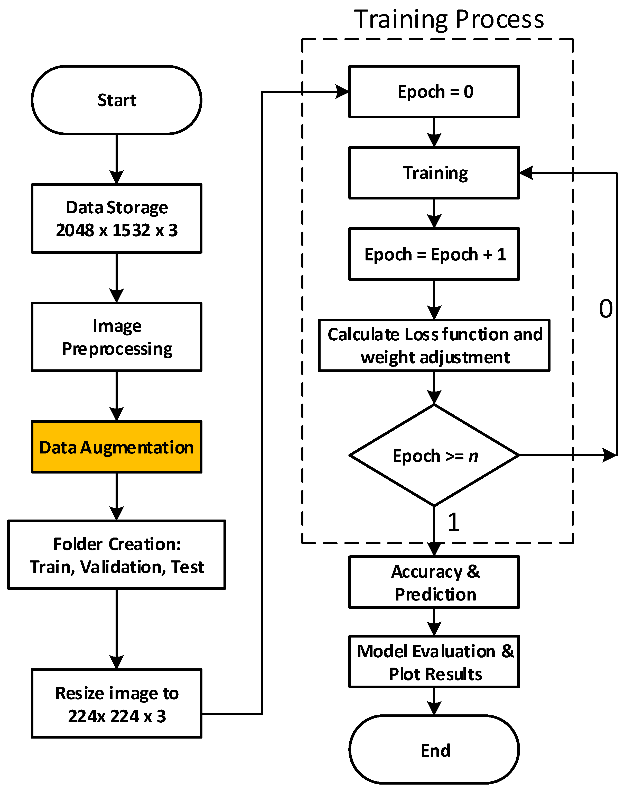
4. Materials and Methods

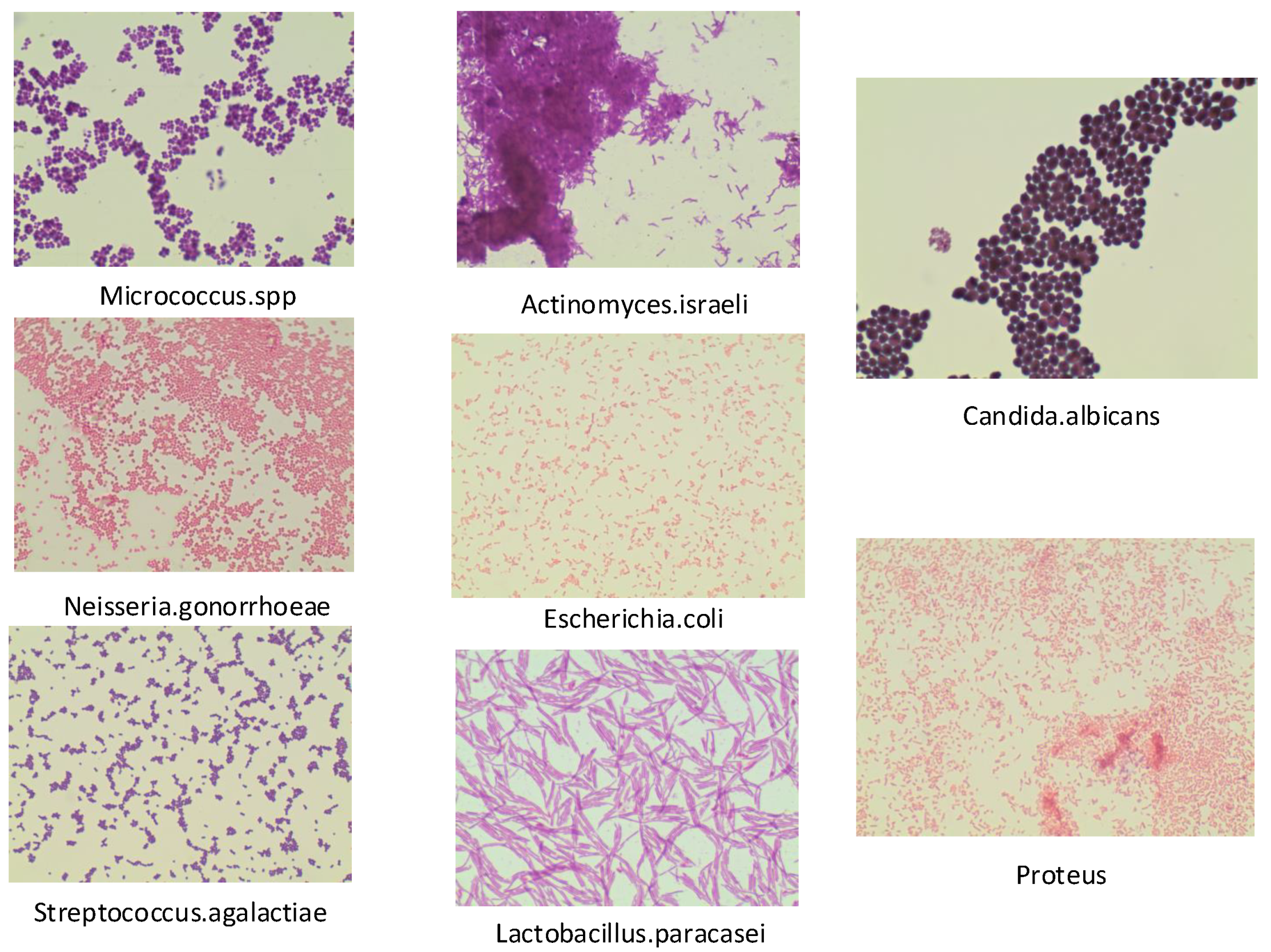
4.1. Dataset

The Digital Images of Bacteria Species dataset [38] consists of 33 bacteria species, each with a total of 20 images in the dataset. The Chair of Microbiology at the Jagiellonian University in Krakow, Poland, was in charge of collecting the samples. Figure 5 shows some of the images captured in this dataset, which have original dimensions of $2048\times 1532\times 3$. All samples were stained using Gram’s process. The images were collected via an Olympus CX31 Upright Biological Microscope paired with an SC30 camera for this project (Olympus Corporation, Japan). Their performance was assessed using a 100-fold objective while submerged in oil (Nikon50, Shinagawa Intercity Tower C, 2-15-3, Konan, Minato-ku, Tokyo 108-6290, Japan). Researchers interested in the bacterial colony domain are able to use the DIBaS dataset on a public-access basis.

Figure 5. Bacteria samples in the DIBaS dataset [38].

4.2. Dataset Augmentation

Deep CNNs are particularly dependent on the availability of large quantities of training data. However, due to the small number of images in the biomedical domain, it is hard to meet the massive input data requirements of CNNs. Another issue when using a small amount of data for CNNs is that it leads to overfitting. A sophisticated solution to alleviate the relative scarcity of the data compared to the number of parameters involved in CNNs is data augmentation [39]. Data augmentation consists of transforming the available data into new data without altering its nature. The computer will detect that the modified model is a different image, but humans still know that the modified image is the same picture. Simple geometric transformations such as sampling [39], mirroring [40], rotating [41], shifting [42], and various photometric transformations [43] are popular augmentation methods.

The number of images in the dataset was significantly increased by using transformations that do not change the classes. Each image was transformed according to the steps mentioned below:

• $rotation\_range$ is a value in the range of $0^0$ to ${180}^0$ within which to rotate pictures randomly; ${40}^0$ was the random value selected;
• $width\_shift=0.2$, and $height\_shift=0.2$ are thresholds (as a fraction of total width or height) within which to randomly shift images vertically or horizontally;
• $shear\_range$ is for randomly employing shearing transformations. It is 0.2;
• $zoom\_range=0.2$ is for randomly zooming the picture sizes;
• $horizontal\_flip$ is for randomly horizontally reversing the pixels of the image;
• $fill\_mode{=}^{\prime }reflec{t}^{\prime }$ is the strategy used for filling in newly created pixels, which can appear after a rotation or a width/height shift.

In addition, some CV functions were exploited in the image augmentation and to open the files in the class folders, as well as save them as .$tif$ files.

As a result, we made 6600 images from the number of original appearances, then utilized histogram equalization techniques to check and maintain the valuable information in the new samples.

5. Experimental Setups

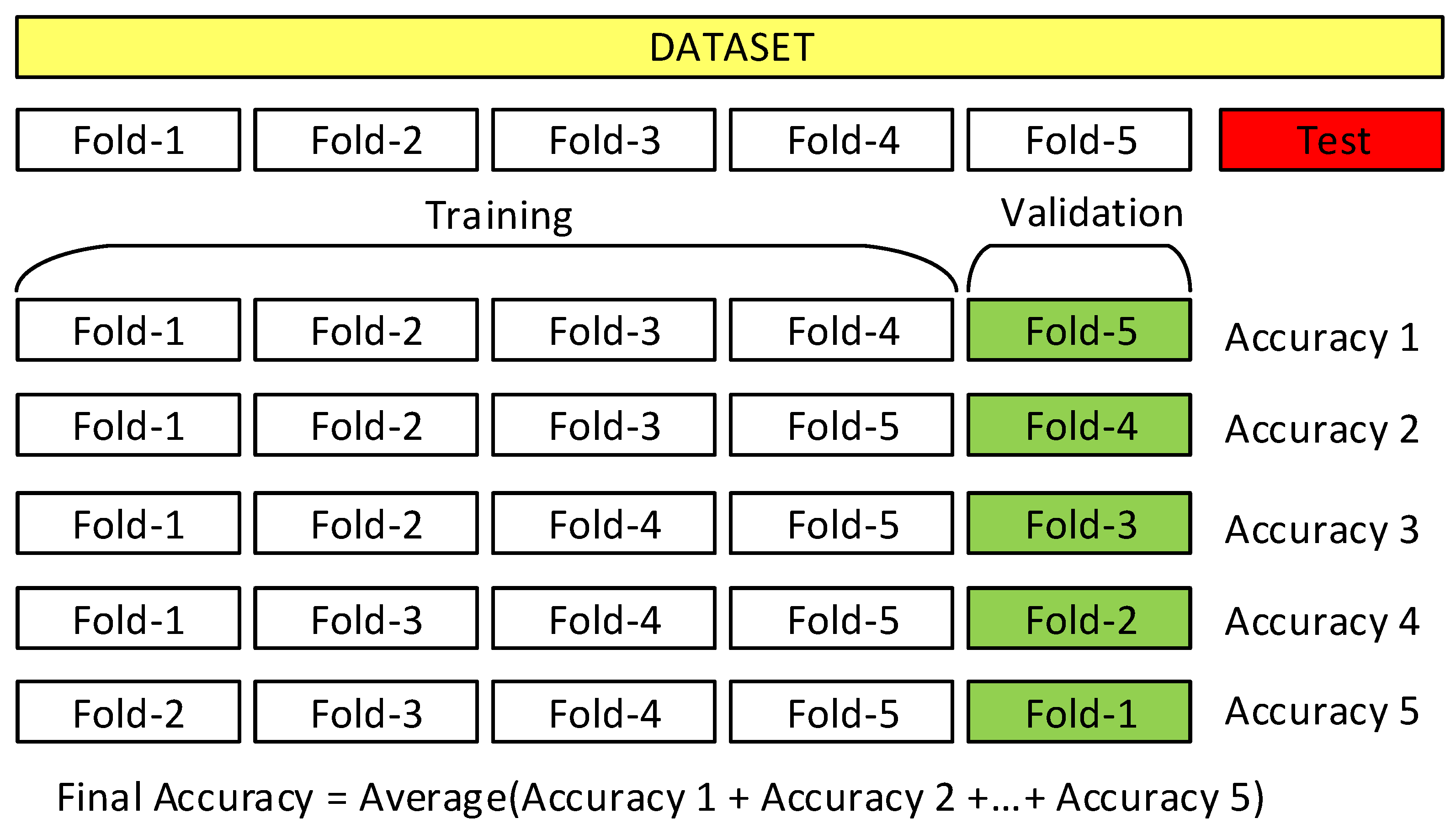
5.1. Training Strategies

Our model was trained and tested on the computational platform of a 64-bit Windows 10 computer with an Intel Core i9 processor (3.6 GHz), 32 GB RAM, and an NVIDIA GeForce RTX 2080 SUPER graphics card. The TensorFlow framework [44] and Keras libraries [45] are the foundations of the Python programming language.

Following preprocessing, the new dataset contained a total of 6600 bacteria images, of which 70% was allocated to the training set and 20% to the validation set and the remainder for test set. The learning rate hyperparameter, which controls the speed of weight update, was set to $\eta =1$ × ${10}^{-4}$, and the weight of the filters was randomly initialized and automatically updated. The experimental setup for the training process is given in Figure 6. The suggested architecture was trained from the scratch.

Figure 6. Research methodology.

5.2. Parameter Selection

The fundamental requirement for proper neural network training is the correct selection of the hyperparameters. For this, we employed grid search optimization on the training set with five-fold cross-validation (Figure 7). We verified some activation functions, including ReLU and sigmoid, for the classifier’s fully (densely) connected layer. The dropout rate, which indicates how many input units are dropped, varied between 0.25 and 0.5. Table 2 lists the parameters that created the most promising results.

Figure 7. Five-fold cross-validation scheme.

Table 2. Hyperparameters and training settings for the suggested models.

Models	Epochs = n	Dropout	Activations Functions	Optimizers	Batch Size
This work	30–50	0.25–0.5	ReLU	Adam	16;32
	30–50	0.25–0.5	ReLU	RMSprop	16;32
	30–50	0.25–0.5	ReLU	Adamax	16;32
	30–50	0.25–0.5	ReLU	Nadam	16;32

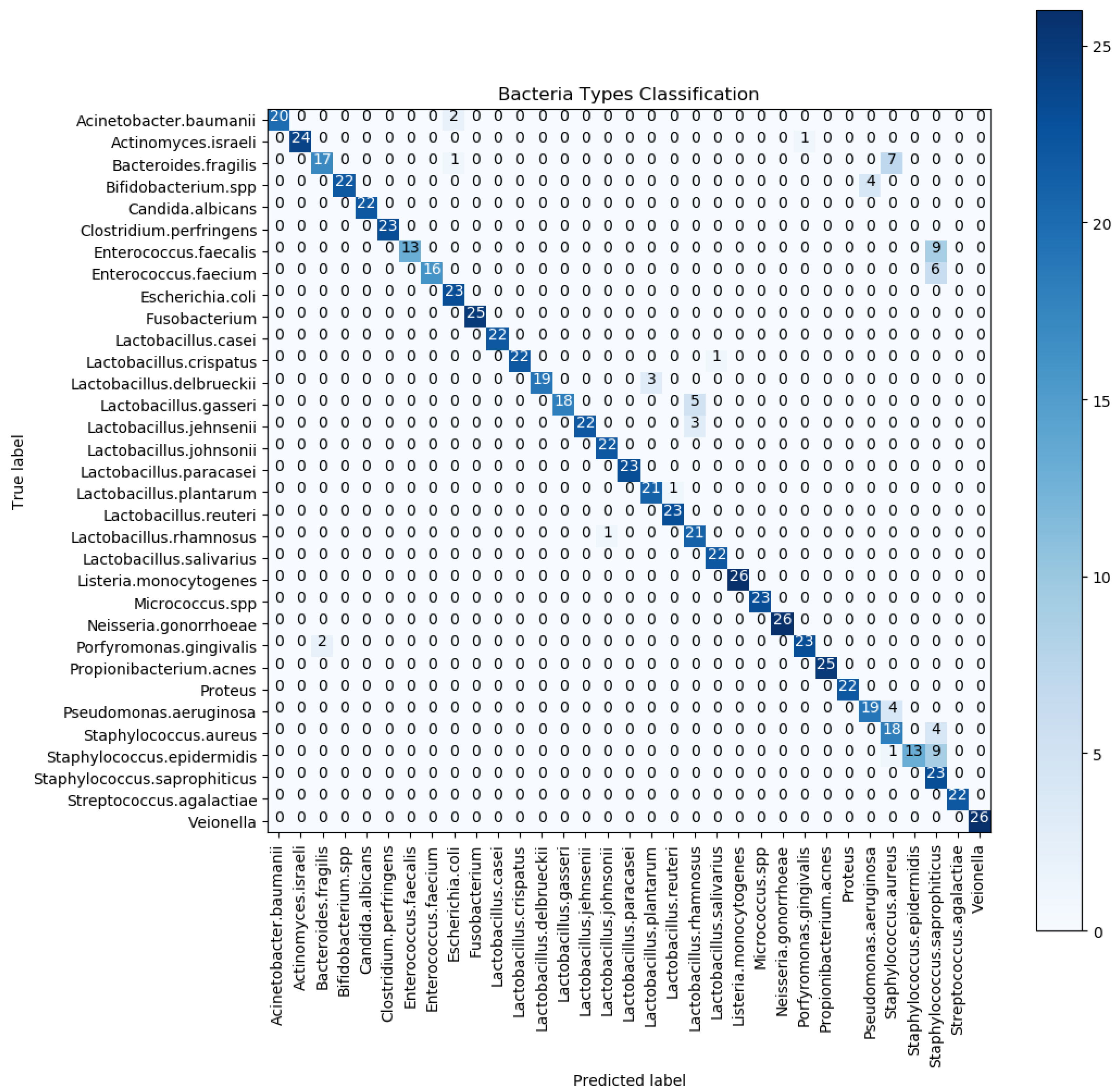
6. Results and Discussion

This section consists of two subsections. In the first subsection, we list some evaluation metrics for the proposed model. Then, we draw a confusion matrix to show the test results on the test set. Finally, a performance comparison table between our method and other studies on the DIBaS dataset is made.

6.1. Statistical Analysis

The evaluation metric plays an essential role in achieving the optimal classifier during the classification training. Thus, determining proper evaluation metrics is a primary key for discriminating against and obtaining the expected results. The model’s performance is often measured using the parameters of accuracy, precision, sensitivity, specificity, and f1 obtained from the confusion matrix (CM) calculation. These metrics, together with the receiver operating characteristic (ROC) curve, area under the curve (AUC), and precision–recall (PR) curve, are widely used as verification standards in machine learning and have been successfully applied in many biomedical studies [46,47,48,49] with high evidence. ROC, AUC, and PR, on the other hand, are better suited to binary classification tasks or a small number of outputs; as a result, they may face significant challenges when describing many outcomes. As a result, in this article, we chose the CM, as well as the accuracy, precision, and F1 as the evaluation metrics.

The values and terms in the CM are shown in Table 3. TP and TN are the correctly classified positive or negative data; FP is negative, but positively classified data; while FN is positive data, but classified as negative. After obtaining the CM values, we calculated the equations’ sensitivity, precision, and F1 indices to evaluate the stated model following several scenarios in Table 2.

Table 3. Confusion matrix values.

Class	Classified Positive	Classified Negative
Positive	TP (True Positive)	FN (False Negative)
Negative	FP (False Positive)	TN (True Negative)

• Accuracy is the most straightforward metric that the model evaluation process requires to quantify a model’s performance. Accuracy is the fraction of correct predictions and the overall number of forecasts. The formula for calculating accuracy is written by:

  $$Accuracy=\frac{(Number\_of\_correct\_predictions)}{(Total\_number\_of\_predictions)};$$

  (11)
• Precision is an evaluation metric that describes a fraction of the true positive prediction and the total number of positive predictions. Precision refers to the frequency with which we are correct when the predicted value is positive:

  $$Precision=\frac{TP}{TP+FP};$$

  (12)
• Sensitivity is the ratio of positive predictions to the total actual number of positives. Sensitivity is also referred to as the recall or true positive rate. Sensitivity means how often the forecast is correct when the real value is positive.

  $$Sensitivity=\frac{TP}{TP+FN};$$

  (13)
• Specificity is calculated by dividing the total number of negative predictions by the total number of actual negatives. Specificity is also understood as the true negative rate. The term “specificity” refers to the frequency with which a prediction is correct when the actual value is negative.

  $$Specificity=\frac{TN}{TN+FP};$$

  (14)
• The $F1$-score, alternatively called the balanced F-score or F-measure, can be calculated as a weighted average of the precision and sensitivity:

  $$F_1=2\times \frac{Precision\times Sensitivity}{Precision+Sensitivity}.$$

  (15)

The detailed performance analysis of the confusion matrix for Fold 5, which was obtained using validation data, is given in Figure 8. The confusion matrix shows that almost all the bacteria images were classified correctly by the recommended pretrained model except for some bacteria images, Enterococcus faecalis, Enterococcus faecium, and Bacteroides fragilis. The model predictions for misclassified bacteria images were Staphylococcus saprophyticus and Staphylococcus aureus, respectively. This mistaken classification can be explained due to the relatively similar color and shape of these bacteria samples and insufficient training images for the model to extract and classify.

Figure 8. Bacteria classification confusion matrix using 5-fold cross-validation.

Table 4 illustrates the comparison of the performance of different optimizers. The most effective choices for data augmentation were the recently popular Nadam and RMSprop, which achieved a maximum of $96.28\%$ accuracy, as well as high precision and sensitivity. Without data augmentation, the optimizers were significantly worse in terms of accuracy, with Adamax and Adam reaching an $86.42\%$ and $86.24\%$ accuracy, respectively.

Table 4. Model performance (%).

Models	Data Aug	Optimizers	Accuracy	Precision	Sensitivity	F1
This work	Yes	Adam	95.01	94.02	90.78	92.37
		Adamax	96.08	94.27	93.22	93.74
		Nadam	96.28	95.81	93.26	94.52
		RMSprop	95.17	95.44	94.84	95.14
This work	No	Adam	86.24	91.11	81.63	86.11
		Adamax	86.42	88.99	83.17	85.98
		Nadam	83.95	85.69	79.26	82.35
		RMSprop	81.48	83.09	75.66	79.21

6.2. Comparison with Other Studies

Figure 9 presents the recent state-of-the-art results conducted on DIBaS image classification.

Figure 9. Recent state-of-the-art studies on DIBaS image classification.

Table 5 depicts a comparison of the results between studies when deployed on the full DIBaS dataset in terms of model structure, number of layers, number of parameters, classification accuracy, and data preprocessing methods. As observed from the figure and table, we concluded that in the present study, the proposed architecture consumed the lowest resources at a bit lower accuracy level compared to the other studies. The analysis suggested that ResNet-50 without using data augmentation had the highest accuracy, while the number of parameters utilized was medium. Nasip et al. and Khalifa et al. announced the same accuracy (∼98.2% ); however, Nasip used many more parameters and input images than Khalifa’s study to obtain these results. It has been proven that the Khalifa method is better than Nasip’s. Our work employed C-Conv and DS-Conv combinations to obtain the same performance (about $96.3\%$) as Zielinski’s work and slightly lower (∼3%) than other works.

Table 5. Comparative analysis among the studies conducted on the DIBaS dataset.

Works	Zielinski et al. [24]	Nasip et al. [25]	Khalifa et al. [28]	M. Talo [26]	S. Patel [31]	This Work
Year	2017	2018	2019	2019	2021	2021
CNN Algorithms	FV, SVM, RF CNNs	VGG-16 AlexNet	AlexNet	ResNet-50	VGG-16	DS-CNN
Layers	8/8/16	16/8	8	50	16	5
Data Augmentation	No	Yes	Yes	No	No	Yes
Transfer Learning	Yes	Yes	Yes	Yes	Yes	No
Number of Images	660	35,600	6600	689	660	6600
Image Dimensions	224 × 224 × 3 227 × 227 × 3	224 × 224 × 3 227 × 227 × 3	227 × 227 × 3	224 × 224 × 3	224 × 224 × 3	224 × 224 × 3
Parameters (M)	58.42 98.95 134.4	134.4	58.42	23.69	134.4	3.23
Accuracy (%)	97.24	98.25	98.22	99.2	93.38	96.28

On the other hand, the parameters (3.23 M) and model size (five layers) of our design were the smallest. The optimization caused it to have convolutional computation and good data augmentation. This approach could pave the way for deep-learning algorithms to be integrated directly in low-resource devices in biomedical fields.

7. Conclusions and Future Work

The experimental results demonstrated that the recommended five-layer DS-CNN architecture has the broad potential to be deployed in medical imaging analysis tasks, especially for small datasets. The CNN variants can improve medical imaging technology further and strengthen its capabilities, providing a higher level of automation while speeding up processes and increasing productivity. This study gained a $96.28\%$ accuracy in bacterial strain classification, as well as the usage of low trainable parameters ($3.23$ M) and less computational complexity ($40.02$ M). This led to consuming less energy and having a slight accuracy tradeoff (∼3%) to fit limited-resource devices.

This algorithm is weakened by the necessity of manually labeled data, massive data and training time requirements to be pretrained, and sometimes the incorrect prediction of the same bacteria species. The network might inherit faults from a specialist, as the correct judgment of a cell is, in many cases, difficult even for an experienced human. A more extensive dataset labeled by a larger group of experts is one solution to mitigate this limitation. Future research will mainly focus on expanding and processing the dataset [50], optimizing the key blocks (DS-Conv) [51], and fine-tuning the last layers. We also plan to implement our dedicated architecture on a hardware platform to utilize robust parallel computation and low energy.

References

1. He, K.; Zhang, X.; Ren, S.; Sun, J. Deep Residual Learning for Image Recognition. In Proceedings of the 2016 IEEE Conference on Computer Vision and Pattern Recognition (CVPR), Las Vegas, NV, USA, 27–30 June 2016; pp. 770–778. [Google Scholar] [CrossRef] [Green Version]
2. Simonyan, K.; Zisserman, A. Very Deep Convolutional Networks for Large-Scale Image Recognition. arXiv 2015, arXiv:1409.1556. [Google Scholar]
3. Simonyan, K.; Zisserman, A. Two-Stream Convolutional Networks for Action Recognition in Videos. arXiv 2014, arXiv:1406.2199. [Google Scholar]
4. Collobert, R.; Weston, J.; Bottou, L.; Karlen, M.; Kavukcuoglu, K.; Kuksa, P. Natural Language Processing (Almost) from Scratch. J. Mach. Learn. Res. 2011, 12, 2493–2537. [Google Scholar]
5. Zhang, T.; Kahn, G.; Levine, S.; Abbeel, P. Learning deep control policies for autonomous aerial vehicles with MPC-guided policy search. In Proceedings of the 2016 IEEE International Conference on Robotics and Automation (ICRA), Stockholm, Sweden, 16–21 June 2016; IEEE: Stockholm, Sweden, 2016; pp. 528–535. [Google Scholar] [CrossRef] [Green Version]
6. Zhou, J.; Troyanskaya, O.G. Predicting effects of noncoding variants with deep learning–based sequence model. Nat. Methods 2015, 12, 931–934. [Google Scholar] [CrossRef] [Green Version]
7. Alipanahi, B.; Delong, A.; Weirauch, M.T.; Frey, B.J. Predicting the sequence specificities of DNA- and RNA-binding proteins by deep learning. Nat. Biotechnol. 2015, 33, 831–838. [Google Scholar] [CrossRef] [PubMed]
8. Zhuang, B.; Shen, C.; Tan, M.; Liu, L.; Reid, I. Structured Binary Neural Networks for Accurate Image Classification and Semantic Segmentation. In Proceedings of the 2019 IEEE/CVF Conference on Computer Vision and Pattern Recognition (CVPR), Long Beach, CA, USA, 16–20 June 2019; pp. 413–422. [Google Scholar] [CrossRef] [Green Version]
9. He, T.; Zhang, Z.; Zhang, H.; Zhang, Z.; Xie, J.; Li, M. Bag of Tricks for Image Classification with Convolutional Neural Networks. In Proceedings of the 2019 IEEE/CVF Conference on Computer Vision and Pattern Recognition (CVPR), Long Beach, CA, USA, 16–20 June 2019; pp. 558–567. [Google Scholar] [CrossRef] [Green Version]
10. Nuriel, O.; Benaim, S.; Wolf, L. Permuted AdaIN: Reducing the Bias towards Global Statistics in Image Classification. In Proceedings of the 2021 IEEE/CVF Conference on Computer Vision and Pattern Recognition (CVPR), Nashville, TN, USA, 19–25 June 2021. [Google Scholar]
11. Nie, D.; Shank, E.A.; Jojic, V. A deep framework for bacterial image segmentation and classification. In Proceedings of the 6th ACM Conference on Bioinformatics, Computational Biology and Health Informatics, Atlanta, Georgia, 9–12 September 2015; pp. 306–314. [Google Scholar] [CrossRef]
12. Ates, H.; Gerek, O.N. An image-processing based automated bacteria colony counter. In Proceedings of the 2009 24th International Symposium on Computer and Information Sciences, Guzelyurt, Cyprus, 14–16 September 2009; pp. 18–23. [Google Scholar] [CrossRef]
13. Divya, S.; Dhivya, A. Human Eye Pupil Detection Technique Using Circular Hough Transform. Int. J. Adv. Res. Innov. 2019, 7, 3. [Google Scholar]
14. Limare, N.; Lisani, J.L.; Morel, J.M.; Petro, A.B.; Sbert, C. Simplest Color Balance. Image Process. Line 2011, 1, 297–315. [Google Scholar] [CrossRef] [Green Version]
15. Ganesan, P.; Sajiv, G. A comprehensive study of edge detection for image processing applications. In Proceedings of the 2017 International Conference on Innovations in Information, Embedded and Communication Systems (ICIIECS), Coimbatore, India, 17–18 March 2017; pp. 1–6. [Google Scholar] [CrossRef]
16. Xuan, L.; Hong, Z. An improved canny edge detection algorithm. In Proceedings of the 2017 8th IEEE International Conference on Software Engineering and Service Science (ICSESS), Beijing, China, 24–26 November 2017; pp. 275–278. [Google Scholar] [CrossRef]
17. Hiremath, P.S.; Bannigidad, P. Automatic Classification of Bacterial Cells in Digital Microscopic Images. In Proceedings of the Second International Conference on Digital Image Processing, Singapore, 26–28 February 2010; 2010; p. 754613. [Google Scholar] [CrossRef]
18. Ho, C.S.; Jean, N.; Hogan, C.A.; Blackmon, L.; Jeffrey, S.S.; Holodniy, M.; Banaei, N.; Saleh, A.A.E.; Ermon, S.; Dionne, J. Rapid identification of pathogenic bacteria using Raman spectroscopy and deep learning. Nat. Commun. 2019, 10, 4927. [Google Scholar] [CrossRef]
19. Kang, R.; Park, B.; Eady, M.; Ouyang, Q.; Chen, K. Single-cell classification of foodborne pathogens using hyperspectral microscope imaging coupled with deep learning frameworks. Sens. Actuators B Chem. 2020, 309, 127789. [Google Scholar] [CrossRef]
20. Sajedi, H.; Mohammadipanah, F.; Pashaei, A. Image-processing based taxonomy analysis of bacterial macromorphology using machine-learning models. Multimed. Tools Appl. 2020, 79, 32711–32730. [Google Scholar] [CrossRef]
21. Tamiev, D.; Furman, P.E.; Reuel, N.F. Automated classification of bacterial cell sub-populations with convolutional neural networks. PLoS ONE 2020, 15, e0241200. [Google Scholar] [CrossRef]
22. Mhathesh, T.S.R.; Andrew, J.; Martin Sagayam, K.; Henesey, L. A 3D Convolutional Neural Network for Bacterial Image Classification. In Intelligence in Big Data Technologies—Beyond the Hype; Peter, J.D., Fernandes, S.L., Alavi, A.H., Eds.; Springer: Singapore, 2021; Volume 1167, pp. 419–431. [Google Scholar] [CrossRef]
23. Korzeniewska, E.; Szczęsny, A.; Lipiński, P.; Dróżdż, T.; Kiełbasa, P.; Miernik, A. Prototype of a Textronic Sensor Created with a Physical Vacuum Deposition Process for Staphylococcus aureus Detection. Sensors 2020, 21, 183. [Google Scholar] [CrossRef]
24. Zieliński, B.; Plichta, A.; Misztal, K.; Spurek, P.; Brzychczy-Włoch, M.; Ochońska, D. Deep learning approach to bacterial colony classification. PLoS ONE 2017, 12, e0184554. [Google Scholar] [CrossRef] [Green Version]
25. Nasip, O.F.; Zengin, K. Deep Learning Based Bacteria Classification. In Proceedings of the 2018 2nd International Symposium on Multidisciplinary Studies and Innovative Technologies (ISMSIT), Ankara, Turkey, 19–21 October 2018; pp. 1–5. [Google Scholar] [CrossRef]
26. Talo, M. An Automated Deep Learning Appoach for Bacterial Image Classification. In Proceedings of the International Conference on Advanced Technologies, Computer Engineering and Science (ICATCES), Karabuk, Turkey, 11–13 May 2019. [Google Scholar]
27. Transfer Learning, CS231n Convolutional Neural Networks for Visual Recognition. Available online: https://cs231n.github.io/transfer-learning/ (accessed on 24 November 2021).
28. Khalifa, N.E.M.; Taha, M.H.N.; Hassanien, A.E. Deep bacteria: Robust deep learning data augmentation design for limited bacterial colony dataset. Int. J. Reason.-Based Intell. Syst. 2019, 11, 9. [Google Scholar] [CrossRef]
29. Plichta, A. Recognition of species and genera of bacteria by means of the product of weights of the classifiers. Int. J. Appl. Math. Comput. Sci. 2020. [Google Scholar] [CrossRef]
30. Plichta, A. Methods of Classification of the Genera and Species of Bacteria Using Decision Tree. J. Telecommun. Inf. Technol. 2020, 4, 74–82. [Google Scholar] [CrossRef]
31. Patel, S. Bacterial Colony Classification Using Atrous Convolution with Transfer Learning. Ann. Rom. Soc. Cell Biol. 2021, 25, 1428–1441. [Google Scholar]
32. Lecun, Y.; Bottou, L.; Bengio, Y.; Haffner, P. Gradient-based learning applied to document recognition. Proc. IEEE 1998, 86, 2278–2324. [Google Scholar] [CrossRef] [Green Version]
33. Sifre, L. Rigid-Motion Scattering for Image Classification. Ph.D. Thesis, Ecole Polytechnique, CMAP, Palaiseau, France, 2014. [Google Scholar]
34. Howard, A.G.; Zhu, M.; Chen, B.; Kalenichenko, D.; Wang, W.; Weyand, T.; Andreetto, M.; Adam, H. MobileNets: Efficient Convolutional Neural Networks for Mobile Vision Applications. arXiv 2017, arXiv:1704.04861. [Google Scholar]
35. Chollet, F. Xception: Deep Learning with Depthwise Separable Convolutions. In Proceedings of the 2017 IEEE Conference on Computer Vision and Pattern Recognition (CVPR), Honolulu, HI, USA, 22–25 July 2017; pp. 1800–1807. [Google Scholar] [CrossRef] [Green Version]
36. Ioffe, S.; Szegedy, C. Batch Normalization: Accelerating Deep Network Training by Reducing Internal Covariate Shift. In Proceedings of the 32nd International Conference on International Conference on Machine Learning, Lille, France, 6–11 July 2015; Volume 37, pp. 448–456. [Google Scholar]
37. Srivastava, N.; Hinton, G.; Krizhevsky, A.; Sutskever, I.; Salakhutdinov, R. Dropout: A Simple Way to Prevent Neural Networks from Overfitting. J. Mach. Learn. Res. 2014, 15, 1929–1958. [Google Scholar]
38. DIBaS—Krzysztof Paweł Misztal. Available online: http://misztal.edu.pl/software/databases/dibas/ (accessed on 24 November 2021).
39. Russakovsky, O.; Deng, J.; Su, H.; Krause, J.; Satheesh, S.; Ma, S.; Huang, Z.; Karpathy, A.; Khosla, A.; Bernstein, M.; et al. ImageNet Large Scale Visual Recognition Challenge. arXiv 2015, arXiv:1409.0575. [Google Scholar] [CrossRef] [Green Version]
40. Yang, H.; Patras, I. Mirror, mirror on the wall, tell me, is the error small? In Proceedings of the 2015 IEEE Conference on Computer Vision and Pattern Recognition (CVPR), Boston, MA, USA, 7–12 June 2015; pp. 4685–4693. [Google Scholar] [CrossRef] [Green Version]
41. Xie, S.; Tu, Z. Holistically-Nested Edge Detection. In Proceedings of the 2015 IEEE International Conference on Computer Vision (ICCV), Santiago, Chile, 7–13 December 2015; pp. 1395–1403. [Google Scholar] [CrossRef] [Green Version]
42. Salamon, J.; Bello, J.P. Deep Convolutional Neural Networks and Data Augmentation for Environmental Sound Classification. IEEE Signal Process. Lett. 2017, 24, 279–283. [Google Scholar] [CrossRef]
43. Eigen, D.; Fergus, R. Predicting Depth, Surface Normals and Semantic Labels with a Common Multi-Scale Convolutional Architecture. arXiv 2015, arXiv:1411.4734. [Google Scholar]
44. Tutorials|TensorFlow Core. Available online: https://www.tensorflow.org/tutorials (accessed on 24 November 2021).
45. Keras documentation: Keras API reference. Available online: https://keras.io/api/ (accessed on 24 November 2021).
46. Le, N.Q.K.; Kha, Q.H.; Nguyen, V.H.; Chen, Y.C.; Cheng, S.J.; Chen, C.Y. Machine Learning-Based Radiomics Signatures for EGFR and KRAS Mutations Prediction in Non-Small-Cell Lung Cancer. Int. J. Mol. Sci. 2021, 22, 9254. [Google Scholar] [CrossRef]
47. Le, N.Q.K.; Hung, T.N.K.; Do, D.T.; Lam, L.H.T.; Dang, L.H.; Huynh, T.T. Radiomics-based machine learning model for efficiently classifying transcriptome subtypes in glioblastoma patients from MRI. Comput. Biol. Med. 2021, 132, 104320. [Google Scholar] [CrossRef] [PubMed]
48. Schneider, P.; Müller, D.; Kramer, F. Classification of Viral Pneumonia X-ray Images with the Aucmedi Framework. arXiv 2021, arXiv:2110.01017. [Google Scholar]
49. Xie, Z.; Deng, X.; Shu, K. Prediction of Protein–Protein Interaction Sites Using Convolutional Neural Network and Improved Data Sets. Int. J. Mol. Sci. 2020, 21, 467. [Google Scholar] [CrossRef] [Green Version]
50. Pei, Y.; Huang, Y.; Zou, Q.; Zhang, X.; Wang, S. Effects of Image Degradation and Degradation Removal to CNN-Based Image Classification. IEEE Trans. Pattern Anal. Mach. Intell. 2021, 43, 1239–1253. [Google Scholar] [CrossRef] [PubMed]
51. Chen, W.; Xie, D.; Zhang, Y.; Pu, S. All You Need Is a Few Shifts: Designing Efficient Convolutional Neural Networks for Image Classification. In Proceedings of the 2019 IEEE/CVF Conference on Computer Vision and Pattern Recognition (CVPR), Long Beach, CA, USA, 15–20 June 2019; pp. 7234–7243. [Google Scholar] [CrossRef] [Green Version]
Publisher’s Note: MDPI stays neutral with regard to jurisdictional claims in published maps and institutional affiliations.
Article Metrics
Citations
Article Access Statistics
Multiple requests from the same IP address are counted as one view.