IoT Dataset Validation Using Machine Learning Techniques for Traffic Anomaly Detection

Abstract

With advancements in engineering and science, the application of smart systems is increasing, generating a faster growth of the IoT network traffic. The limitations due to IoT restricted power and computing devices also raise concerns about security vulnerabilities. Machine learning-based techniques have recently gained credibility in a successful application for the detection of network anomalies, including IoT networks. However, machine learning techniques cannot work without representative data. Given the scarcity of IoT datasets, the DAD emerged as an instrument for knowing the behavior of dedicated IoT-MQTT networks. This paper aims to validate the DAD dataset by applying Logistic Regression, Naive Bayes, Random Forest, AdaBoost, and Support Vector Machine to detect traffic anomalies in IoT. To obtain the best results, techniques for handling unbalanced data, feature selection, and grid search for hyperparameter optimization have been used. The experimental results show that the proposed dataset can achieve a high detection rate in all the experiments, providing the best mean accuracy of 0.99 for the tree-based models, with a low false-positive rate, ensuring effective anomaly detection.

1. Introduction

Given the growth and wide implementation of Internet of Things (IoT) networks in different areas, it has taken a significant role in our daily activities, evolving as the driving force behind home automation, smart cities, modern health systems, and advanced manufacturing [1]. However, with advancements in engineering and science, the application dimensions of smart systems are increasing, generating a faster growth of the IoT network traffic that also raises concerns about security vulnerabilities and limitations. The Internet and its users are already under continuous intrusions that can be exhibited as traffic anomalies, representing a threat to the IoT as a set of many restricted devices. This fact can cause different points of view that generate new and ingenious malicious models. The challenge is to prevent the growth of such models or at least to mitigate and limit their impact [2].

The anomalies in a network cannot always be categorized as an attack and are not always harmful elements; even so, they provide important insights into traffic behavior and can help to identify important and critical information in various applications [3]. One way to recognize alterations in the behavior of the network is through Intrusion Detection Systems (IDSs), which help to discover, determine, and identify the unauthorized use, duplication, alteration, and destruction of information systems. Traditional IDS methods are less effective or insufficient for the security of IoT systems because of their peculiar characteristics such as limited energy, ubiquity, heterogeneity, limited bandwidth capacity and global connectivity [4]. In fact, IoT introduces the need for specialized standards and communication protocols to handle typical resulting challenges. At the transport layer, TCP and UDP are the dominant protocols for most of the applications. However, these functions should be implemented in interoperable standard ways, and several message distribution functions are needed depending on IoT application requirements. The MQTT protocol is often used for publishing and/or subscribing messages received from low bandwidth devices across untrusted networks. MQTT operates over TCP for sending and receiving the middleware data to IoT hubs.

In order to mitigate traffic anomalies, the developers need to enhance new techniques to detect affected IoT devices. Machine learning (ML) Anomaly-based techniques have recently gained credibility in a successful application for the detection of network anomalies including IoT networks. This is because ML-based methods can capture and examine benign and anomalous IoT traffic. Anomaly-based detection techniques using supervised machine learning rely on a baseline normal/anomalous behavior profile for the monitored environment. This baseline is then used for comparing system actions and taking decision over the network events. Furthermore, ML-based methods have been tested to predict new or zero-day attacks. Hence, ML-based algorithms provide robust security protocols for designing the security of IoT devices and networks [4].

A crucial aspect is that ML cannot work without representative data, and the correctness of the collected data from the devices is necessary to make intelligent decision systems, as well as effectively managing IoT environments. Supervised methods (also known as classification methods) required a labeled training set containing both normal and anomalous samples to construct the predictive model. Theoretically, supervised methods provide a better detection rate than semi-supervised and unsupervised methods, since they have access to more information. The most common supervised algorithms are Neural Networks, Support Vector Machines, k-Nearest Neighbors, Bayesian Networks, and Decision Trees [5].

1.1. Motivation

Due to the interconnected and interdependent settings of the IoT, this environment is vulnerable to different security and privacy issues, which may cause unauthorized tasks to be performed by the remote malicious users [6], and therefore, abnormal behavior on the network. In other cases, anomaly traffic on an IoT network may come from a wrong configuration, abnormal installation or a hardware malfunction of the sensors.

Consequently, there is a demand to research specific detection and prevention techniques and design and develop intelligent security solutions for the protection of vulnerable IoT devices and against anomalies generated by compromised IoT devices. The creation of anomaly IDSs requires representative knowledge of the environment.

Given the scarcity of IoT datasets, the DAD [7] emerged as a mechanism to know the behavior of dedicated, lightweight devices, IoT-MQTT networks. The DAD dataset [7] is a complete and labeled MQTT-IoT dataset for real-world traffic anomaly detection, in suitable conditions, with sufficient trace size, diverse anomaly scenarios, with previous analysis and intended to be applied on ML. However, the dataset must be subject to the application of machine learning models to confirm its applicability for the purpose for which it was conceived.

1.2. Contributions of the Work

This work aims to demonstrate that the DAD dataset can be used to detect anomalies in MQTT-IoT traffic networks, applying five widely used shallow learning techniques for traffic anomaly detection in IoT environments. The main contributions of this research are:

• Analysis and extraction of characteristics for IoT wireless sensor networks;
• Implementation of data conditioning techniques, for binning, handling unbalanced data and feature extraction in real environments;
• Application of different machine learning algorithms to validate the selected dataset;
• Application of metrics and performance comparison of the different machine learning techniques in the detection of traffic anomalies.

1.3. Paper Organization

This work is structured as follows. The review of the intrusion detection systems using machine learning techniques for IoT networks is discussed in Section 2. Section 3 presents a short definition of the selected algorithms, besides the parameters chosen to perform the hyperparameter tuning. Section 4 exposes a brief disclosure of the scenario, describing, exploring and verifying data quality contained in the dataset. Then, raising the data quality to the level required by the machine learning techniques selected is mandatory. Section 5 introduces the techniques and the process required by the data to be perfectly intelligible to ML algorithms. Section 6 analyzes the results obtained for each of the models in the training stage. Consequently, Section 7 discusses the results obtained during the test stage, as well as performing a comparison between the models. Finally, Section 8 illustrates the main conclusions of this work.

2. Related Work

The relatively effortless implementation and the results achieved in IDSs that employ machine learning algorithms have made many researchers choose these techniques as a development instrument in their projects. However, the application of IDSs in IoT has been a widely disseminated task recently. This section exposes a brief disclosure of the most relevant machine learning techniques employed to validate IoT datasets in recent years.

Given the initial lack of specific IoT public datasets, the application of IDSs in this environment began fitting generic datasets, widely accepted by the community, to IoT network traces. The most commonly adopted dataset in IoT has been the UNSW-NB15 dataset [8], so that several researchers have tested their machine learning applications to this dataset. Koroniotis et al. [9] enforce four classification techniques, Decision Tree (DT), Association Rule Mining (ARM), Artificial Neural Network (ANN), and Naive Bayes (NB), validating the capacity of the algorithms for the recognition of attack vectors. AD-IoT [10] also selected one part of the UNSW-NB15 dataset and proposes an anomaly detection system for detecting cyberattacks at fog nodes in a smart city based on ensemble methods, using Random Forest (RF) and Extra Tree (ET) bagging techniques. In addition, the UNSW-NB15 and NIMS botnet datasets with simulated IoT sensors data were used by Moustafa et al. [1] to perform a Network Intrusion Detection System (NIDS) based on an AdaBoost ensemble learning algorithm using three machine learning techniques—DT, NB and ANN.

On the other hand, Pajoouh et al. [11] used the NSL-KDD dataset and proposed a model that applies a two-tier classification module utilizing Naive Bayes (NB) and the Certainty Factor version of K-Nearest Neighbor to identify malicious activities such as User to Root (U2R) and Remote to Local (R2L) attacks.

With the proliferation of the application of IoT environments, the demand for specialized IDS increased, and, consequently, the need for the publication of dedicated datasets, which would allow the validation of the systems.

Kitsune [12] is a system for network intrusion detection, uses an ensemble of Neural Networks called autoencoders to differentiate between normal and abnormal traffic patterns, which was developed by applying the N-BaIoT [13] dataset. N-BaIoT builds and collects traffic from two networks: a video surveillance network with IP cameras where they launched eight different types of attacks that affect the availability and integrity of video links. The second one was an IoT network consisting of three PCs and nine IoT devices, infected with the Mirai botnet malware. Furthermore, Abbasi [14] employs this dataset for classification using Logistic Regression (LR) and Artificial Neural Network (ANN).

Doshi et al. [15], based on the fact that the IoT traffic is often distinct from that of other Internet-connected devices, develop a machine learning pipeline, designing features to capitalize on IoT-specific network behaviors. The pipeline is developed to operate on network middleboxes (e.g., routers, firewalls, or network switches) to identify anomalous traffic and corresponding devices that may be part of an ongoing botnet. In this work, the authors compare a variety of classifiers for attack detection, including the K-nearest neighbors “KDTree” algorithm (KNN), Support Vector Machine with linear kernel (LSVM), Decision Tree using Gini impurity scores (DT), Random Forest using Gini impurity scores (RF) and Neural Network (NN), demonstrating the effectiveness of Random Forest.

Basing their work on the IoT-specific dataset published by Pahl et al. [16], Hasan et al. [17] proposed a smart, secured and reliable machine learning system, using LR, SVM, DT, RF, and ANN. The IoT based infrastructure exploited several classifiers, which can detect and protect the system when it is in an abnormal state, obtaining the best performance with RF and ANN in training and testing accuracy. Unfortunately, the dataset has only one day of traffic capture.

Koroniotis et al. [18] who had already developed work on the application of machine learning in IDS, design a specific botnet dataset in IoT called Bot-IoT, to confirm the effectiveness of the techniques in this environment. The structure incorporates both normal IoT-related and other network traffic, along with various types of attack traffic commonly used by botnets. It contains attack categories and subcategories for possible multiclass classification purposes. They apply algorithms of Support Vector Machine (SVM), Recurrent Neural Network (RNN) and Long-Short Term Memory Recurrent Neural Network (LSTM-RNN) to compare the validity and evaluate the dataset accuracy. Likewise, other authors as Susilo et al. [19] and Alsamiri [20] based their experiments on exploiting the Bot-IoT dataset. Susilo built an anomaly detection system applying RF, SVM, MLP, and CNN, while Alsamirimi implemented NB, RF, MLP, Iterative Dichotomiser 3 (ID3), AdaBoost, Quadratic discriminant analysis (QDA), and KNN.

Anthi et al. [21] propose a three-layer Intrusion Detection System (IDS) generating a representative dataset that uses a supervised approach to detect a range of popular network-based cyber-attacks on IoT networks. For the validation of potential intrusion detection systems, they considered NB, Bayesian Network, J48, Zero R, OneR, Simple Logistic, SVM, MLP, and RF. However, the dataset employed does not use specific IoT protocols and only contains two days of anomaly traffic capture.

The MedBIoT [22] provides a labeled behavioral IoT dataset, incorporating normal and botnet malicious network traffic. The proposed scenario is a medium-sized IoT network infrastructure (83 IoT devices), composed of common real and emulated IoT devices, combining three prominent botnet malware (Mirai, BashLite, and Torii). Machine learning classification models (KNN, SVM, DT, and RF) were implemented, verifying the applicability of the proposed dataset.

Thamaraiselvi et al. [23] employed algorithms such as RF, NB, SVM, and DT to detect anomalies in IoT networks. To perform their experiments, they exploited the IoT-23 [24], which offers a large dataset consisting of twenty-three captures of different IoT network traffic. These scenarios were divided into twenty network captures from infected IoT devices and three network captures of real IoT devices network traffic. Malware captures are executed for long periods, performing diversity attack scenarios, including Mirai, Torii, and Gagfyt.

An application for IIoT was found in [25]. Machine learning-based anomaly detection algorithms are employed to find malicious traffic in a synthetically generated dataset of Modbus/TCP communication of a fictitious industrial scenario. The dataset contains common home and office-based penetration attacks mimicking the timing behavior and the rate of packets per time unit, which is a good distinguishing factor for attacks. Four different machine learning algorithms were used to detect anomalies: SVM, RF, KNN, and k-means clustering. The best outcomes were achieved with the Support Vector Machine.

Liu et al. [26] created a publicly available dataset using smart sensors in an IoT network. The data was collected in the smart lab and smart home environments using Rainbow HAT sensor boards installed on Raspberry Pis. The dataset contains five types of cyberattacks: Address Resolution Protocol (ARP) Poisoning, ARP Denial-of-Service (DoS), UDP Flood, Hydra Bruteforce with Asterisk protocol, and SlowLoris. They proposed a hybrid method that combines an embedded model for feature selection and a CNN for attack classification. The proposed intrusion detection method has two models: (a) RCNN, where Random Forest is combined with a convolutional neural network (CNN); and (b) XCNN, where eXtreme Gradient Boosting (XGBoost) is combined with CNN. A hybrid technique which is a combination of fog computing and cloud computing is adopted. Additionally, they probe the classifications on CCD-INID-V1 and two other IoT datasets, the N_BaIoT dataset [13] and the CIRA-CIC-DoHBrw-2020 dataset (DoH20) [27], to explore the effectiveness of these learning-based security models and compare the effectiveness of their proposed technique to traditional ML algorithms, such as KNN, NB, LR, and SVM, providing the comparative results of anomaly and multiclass classifications.

Vaccari et al. presented MQTTset [28], a dataset focused on the MQTT protocol composed of IoT devices of different nature (e.g., temperature, humidity, motion sensors, etc.), to simulate a smart home/office/building environment. MQTTset combines legitimate traffic with different malicious/attack traffic such as flooding denial of service attacks, MQTT Publish flood, SlowITe, malformed data, and brute force authentication, to replicate different contexts such as home automation, monitoring of critical infrastructures or industrial contexts. Based on this scenario, they perform an intrusion detection system implementing DT, RF, MLP, NN and Gaussian NB to identify malicious behaviours, in order to protect the system from attacks.

Most of the works performed in NIDS seek to obtain feature extraction and a set of algorithm combinations that optimize results. Sarhan et al. [29] sought to standardize the techniques so that they could apply to any dataset. For their experiments, they used six machine learning models: Deep Feed Forward (DFF), CNN, Recurrent Neural Network (RNN), DT, LR, and NB. They also explored three algorithms for the extraction of characteristics, Principal Component Analysis (PCA), Linear discriminant analysis (LDA), and Auto-encoder (AE), in three benchmark datasets, UNSW-NB15 [8], ToN-IoT [30], and CSE-CIC-IDS2018 [31]. The results obtained indicate that there is no definite feature extraction method or ML model that can achieve the best scores for all datasets, and the choice of datasets significantly alters the performance of the applied techniques.

Machine learning techniques were initially applied to datasets not belonging to IoT networks, adjusting traces to this environment, demonstrating that these techniques can be applied for detecting attacks in this type of scenario. The appearance of specific IoT datasets allows to model real environments, ensuring the optimal application of machine learning algorithms for validation of existing datasets. After reviewing the main techniques used to detect traffic anomalies using ML, focused on IoT environments, we decided to choose five different machine learning models of different natures to validate the DAD dataset: Logistic Regression, Naive Bayes, Random Forest, Adaboost, and Support Vector Machines.

3. Machine Learning Techniques

Machine learning is about extracting knowledge from data. The most successful kinds of machine learning algorithms are those that automate decision-making processes by generalizing from known examples. This is known as supervised learning [32]. Of the many machine learning methods, some are less flexible, or more restrictive, being the shallow models simpler in the sense that they can produce just a relatively small range of shapes to estimate.

Generally, to build a high accuracy classification model, it is very important to choose a powerful machine learning algorithm as well as to adjust its parameters. Most machine learning algorithms achieve optimal results if their parameters are tuned properly. Inappropriate parameter settings lead to poor classification results. Parameter optimization can be very time-consuming if done manually especially when the learning algorithm has many parameters. Hence, the grid search is originally an exhaustive search based on a defined subset of the hyper-parameter space. Grid search optimizes the model parameters using a cross-validation (CV) technique as a performance metric. The goal is to identify a good hyper-parameter combination so that the classifier can predict unknown data accurately. The cross-validation technique can prevent the over-fitting problem [33].

As already mentioned, to perform the experimentation, have been selected five supervised shallow learning classification algorithms of different nature: Logistic Regression, Naive Bayes, Random Forest, Adaboost, and Support Vector Machines. A concise explanation of each algorithm is done, followed by a short description of the hyperparameters considered for tuning.

The first machine learning model considered is Logistic Regression, which is a statistical method that allows the analysis and prediction of a binary outcome. This machine learning model is a specific case of a set of generalized linear models. The objective of Logistic Regression is to create the best fitting model to establish a relationship of dependence between the class variable and the features [34]. This model does not really have any critical hyperparameters to tune. Even so, L1, L2, and C parameters can be tuned as regularization techniques to address over-fitting. L1 regularization technique handles a Lasso Regression model, while L2 operates over a Ridge Regression model. In short, L1 regularization tries to estimate the median of the data, while L2 regularization tries to estimate the mean of the data. The C parameter is the inverse regularization parameter. It is a control variable that retains the strength modification of regularization by being inversely positioned to the Lambda regulator. Higher values of C correspond to less regularization to avoid over-fitting the model.

The Naive Bayes model is a heavily simplified Bayesian probability model, which operates on a strong independence assumption. This means that the probability of one attribute does not affect the probability of the other. Given a series of n attributes, the Naive Bayes classifier makes $2n!$ independent assumptions. Nevertheless, the results of the Naive Bayes classifier are often correct [35]. Naive Bayes classifiers are a family of classifiers that are quite similar to Logistic Regression and Linear Support Vector Classifier (SVC). However, they tend to be even faster in training. The price paid for this efficiency is that Naive Bayes models often provide a generalization performance that is slightly worse than that of linear classifiers. The reason that Naive Bayes models are so efficient is that they learn parameters by looking at each feature individually and collect simple per-class statistics from each feature. For binary data classification, the Bernoulli Naive Bayes is employed. This classifier assumes binary data counts how often every feature of each class is not zero. Bernoulli NB has a single parameter, $\alpha$, which controls model complexity. The way $\alpha$ works is that the algorithm adds to the data $\alpha$ many virtual data points that have positive values for all the features. This results in a “smoothing” of the statistics. A large $\alpha$ means more smoothing, resulting in less complex models. The algorithm’s performance is relatively robust to the setting of $\alpha$, meaning that setting $\alpha$ is not critical for good performance [36].

On the other hand, the tree-based models have been providing a notable performance on their applications in the realm of behavior-based Intrusion Detection Systems. Random Forest (RF) builds multiple Decision Trees without pruning, induced by bootstrapping samples of the training data, using a selection of random features. Prediction is made by aggregating (majority vote for classification or averaging for regression) the calculations of the set. Random Forest generally exhibits a substantial improvement in performance over the single tree and provides a low error rate with an exceptional noise resistance [32]. The n_estimators parameter indicates the number of trees to grow in the RF model. A larger number of trees produces more stable models, but requires more memory and a longer run time. The max_features parameter refers to the number of features to consider when looking for the best split. We have considered $sqrt$ (that is, sqrt(n_features)) and $log2$ (that is, log2(n_features)) as possible values for this parameter.

The AdaBoost (short for Adaptive Boosting) is a stereotype algorithm of boosting, whose basic idea is to select and combine a group of weak classifiers to form a strong classifier. Boosting algorithm is adopted as a repetitive approach for producing a robust classifier, achieving a randomly small training error, from weak classifiers ensembled only from random guessing. Ensemble is employed to draw training records by repeatedly updating the sample distribution of the data that have been trained [37]. The base estimator used in this implementation is a Decision Tree classifier. For hyperparameter tuning the n_estimators parameter performs the maximum number of estimators at which boosting is terminated. In the case of a perfect fit, the learning procedure is stopped early. The learning_rate parameter is provided to shrink the contribution of each classifier, that is the weight applied to each classifier at each boosting iteration. A higher learning rate increases the contribution of each classifier. There is a trade-off between the learning_rate and n_estimators parameters.

The latest supervised technique on the scene is Support Vector Machine (SVM). SVM transforms the data into higher dimensions and finds the hyperplane that best separates the data. A Support Vector Machine classifies data by finding the best hyperplane that separates all data points of one class from those of the other class. SVMs revolve around the notion of a “margin” on either side of a hyper-plane that separates two data classes. Margin means the maximal width of the slab parallel to the hyperplane that has no interior data points. Maximizing the margin and thereby creating the largest possible distance between the separating hyper-plane and the instances on either side of it has been proven to reduce an upper bound on the expected generalization error [38]. The kernel controls how the input variables will be projected. There are many to choose from, but linear, polynomial, and RBF are the most common. When an SVC employs a linear kernel for classification, it can be defined as a Linear SVC. Linear models can be quite limiting in low-dimensional spaces, as lines and hyperplanes have limited flexibility. One way to make a linear model more flexible is by adding more features. A critical parameter is the C penalty regularization parameter that can take on a range of values and has a dramatic effect on the shape of the resulting regions for each class. A log scale might be a good starting point. The strength of the regularization is inversely proportional to C, so it must be strictly positive. As with the linear models, a small C means a very restricted model, where each data point can only have very limited influence [36].

4. Dataset Overview

To apply Machine Learning techniques, it is necessary to have a dataset with a considerable number of samples, contextualized and correctly labeled. This section presents a brief description of the scenario in which the selected dataset was developed. Then, a summarized analysis of the relevant data for the classifier. A detailed analysis of the dataset can be found in [39].

4.1. Scenario Description

To approximate the dataset to a real environment, data were obtained from temperature sensors in the CITIC data center [40]. The dataset, called DAD, presents seven days of the situation that occurs daily in a real environment with sufficient trace size and with a concrete feature extraction presented.

The sensors monitor the temperatures of the data center over three elements: the racks, the power strips (PDU), and the refrigeration machines (InRow). We only considered the sensors of the InRows, because the values of the rest of the sensors are static, and not meaningful. The most important devices of the system are the InRows (13, 15, 23 and 25), responsible for cooling the air of the data center through a liquid cooling system. The InRows have four relevant sensors: (i) unit supply air temperature (TAS); (ii) unit return air temperature (TAR); (iii) unit entering fluid temperature (TFEU); and (iv) unit leaving fluid temperature (TFSU).

Regarding the virtualized environment, five virtual machines with Ubuntu server 18.04 operating system were created, each of them connected to the internal IoT network, so the traffic between them is totally isolated.

There are four sensors in each of the four refrigeration units. Every client node launches a process that simulates every sensor with an identifier correlated with the cold unit identifier (InRow). For example, cold unit 13 has stamped 131 for TAS, 132 for TAR, 133 for TFEU, and 134 for TFSU. Once the sensor is connected for publication of the corresponding topic to the broker, the sensor sends an MQTT message with its identifier node as ClientId. Every InRow sensor has the same IP address, but the ports used for message transmission are different for individual sensors every day. Because of this, a total of 112 TCP ports are utilized. Each of these sensors sends data to the broker every five minutes, that is, 288 samples per hour, for a total of 4032 samples per sensor every day. The sensors do not make connections between themselves.

The dataset presents diverse sets of anomaly scenarios where abnormal traffic is statistically different from normal traffic, being the majority of network traffic instances normal. It is labeled at packet level, indicating the type of token (normal or anomaly).

The behavior of the anomaly node has been modified in one of the following ways:

• Interception: randomly deleting some sent packets.
• Modification: changing the temperature to be sent, without following the established pattern.
• Duplication: sending more tokens than the number initially planned.

4.2. Content Description

Numerical data are analyzed in order to understand the conceptual model of the observed values. The anomaly traffic is made from InRow 13 with IP source 10.6.56.41, where the anomaly packets have been released on specific days of the week (on Wednesday, Thursday, Friday and Saturday). DAD has a total of 101,583 packets, UDP and TCP being the prevalent traffic. Of the packets, 63.3% belong to MQTT traffic and 16% of these are marked as anomalies. The number of source bytes, destination bytes, source packets, destination packets, TCP packets, UDP packets and MQTT packets is uniform throughout the days of the week, presenting an average of 14,020 TCP packets, of which 9267 are MQTT packets per day.

The intercept anomalies are not labeled in the dataset, because these packages have been eliminated. The interception packages do not exist, which is why they are not reflected in the general statistics as abnormal packages. In other words, the anomalous traffic percentages do not take the interception anomalies into account.

Every sensor sends messages to the broker every 5 min. An idle timeout of 30 s was configured, so, if a node stops sending packets for this period, the next packet is considered part of a new flow. Flows were established as unidirectional. Due to the type of connection typical of MQTT networks, alteration in one of the sensor messages affects the entire MQTT flow. As a result, if a packet belongs to a flow where at least a packet is labeled anomaly, all the flow packets are considered abnormal.

The dataset has a total of 224 TCP connection flows of which 208 represent normal flows and 16 anomaly flows. In addition, it presents 67,848 MQTT flows, of which 544 correspond to anomaly flows. The number of flows throughout the days is homogeneous, presenting a smaller number on Sunday due to connection closures that are made the next day. All anomalies are performed on TCP flows.

5. Data Preparation

As a stage prior to the application of the machine learning algorithms, the data, instances and attributes used for the analysis have to be exposed. This task involves raising the data quality to the level required by the analysis techniques selected, considering transformations of the data and constructions from one or more existing attributes made for cleaning purposes and their possible impact on the analysis results.

It is important to know the parameters that machine learning algorithms need to adapt for optimal execution. Knowing the nature and operation of the classifier, 14 attributes are considered relevant and selected for processing:

‘‘ip.src.’’, ‘‘tcp.srcport.’’, ‘‘frame.len’’, ‘‘frame.time’’,

‘‘ip.dst’’, ‘‘tcp.dstport’’, ‘‘tcp.flags’’, ‘‘tcp.flags.ack’’,

‘‘tcp.flags.fin’’, ‘‘tcp.flags.res’’, ‘‘tcp.flags.reset’’,

‘‘tcp.flags.syn’’,  ‘‘protocol’’, ‘‘label’’.

New attributes are created for a better estimation of the model:

• Weekday: the day of the week extracted from frame.time.
• Protocol\_Type: determines if it is an MQTT-IoT protocol.
• ClientID: it is the attribute that allows to identify which sensor of the InRow it belongs to, based on ip.src and tcp.srcport attributes.

Some data are cyclical by default. This is the case of hours, minutes and seconds. If we take the hour as a linear variable, the classifier does not understand that hour 23 precedes hour 0. To solve this problem, cyclical values must be given to the Machine Learning algorithm, replacing the existing attribute with two new features using the sine representation. You need both variables or the proper movement through time is lost. This is due to the fact that the derivative of either sine or cosine changes in time where the (x,y) position varies smoothly as it travels around the unit circle.

For a 24 h clock this is achieved with sine and cosine transforms, respectively, as in Equation (1).

$$\begin{gathered} x=\mathit{sin}(2\ast \pi \ast \mathit{hour}/24) \\ y=\mathit{cos}(2\ast \pi \ast \mathit{hour}/24). \end{gathered}$$

(1)

The distance between two points corresponds to the difference in time, as we expect from a 24-h cycle.

As previously mentioned, due to the connection in the dataset, 112 TCP have been used. For the mapping, this situation implies the construction of 112 attributes with redundant information implicit in the ClientId. Seeing this, the features of the tcp.srcport and tcp.dstport are discarded.

The best way to represent data depends not only on the semantics of the data, but also on the kind of model we are using. Linear models and tree-based models (such as Decision Trees, Gradient Boosted Trees, and Random Forests), two large and very commonly used families, have very different properties when it comes to how they work with different feature representations. Linear models can only model linear relationships, which are lines in the case of a single feature. One way to make linear models more powerful on continuous data is to use binning (also known as discretization) of the feature to split it up into multiple features. Here, and as a process common to all the models, a single continuous input feature of the dataset is transformed into a categorical feature that encodes which bin a data point is in [36]. The categorical features in the dataset must be converted into a numeric representation. This process is done by the usual binary encoding, where each categorical variable having possible m values is replaced with m − 1 dummy variables. Here, a dummy variable has a value of one for a specific category and zero for all the remaining categories [41].

Regarding the label feature, the normal class is mapped to a numeric value of 0 and the anomaly class is mapped to a numeric value of 1. The frame time attribute is converted into a date variable to be able to extract other relevant information from this. The feature d_flow represents the duration of the flow and frame.len_mean corresponds to the arithmetic mean of the frame length of all packets belonging to the flow. We transform all to discrete features. The resulting attributes were:

[‘frame.len’, ‘hora_cos’, ‘hora_sin’, ‘Npackperflow’, ‘d_flow’,

‘tcp.flags.ack’, ‘tcp.flags.fin’, ‘tcp.flags.reset’, ‘tcp.flags.syn’,

‘frame.len_mean’, ‘tcp.flags.res’, ‘label_fl’,

‘ip.src_10.6.56.1’, ‘ip.src_10.6.56.34’, ‘ip.src_10.6.56.36’,

‘ip.src_10.6.56.41’, ‘ip.src_10.6.56.50’, ‘ip.dst_10.6.56.1’,

‘ip.dst_10.6.56.34’, ‘ip.dst_10.6.56.36’, ‘ip.dst_10.6.56.41’,

‘ip.dst_10.6.56.50’, ‘ClientId_131’, ‘ClientId_132’, ‘ClientId_133’,

‘ClientId_134’, ‘ClientId_151’, ‘ClientId_152’, ‘ClientId_153’,

‘ClientId_154’,

‘ClientId_231’, ‘ClientId_232’, ‘ClientId_233’, ‘ClientId_234’,

‘ClientId_251’, ‘ClientId_252’, ‘ClientId_253’, ‘ClientId_254’,

‘ClientId_Broker’, ‘protocol_TIP_MQTT’, ‘protocol_TIP_TCP’,

‘weekday_Friday’, ‘weekday_Monday’, ‘weekday_Saturday’,

‘weekday_Sunday’, ‘weekday_Thursday’, ‘weekday_Tuesday’,

‘weekday_Wednesday’]

After mapping symbolic attributes to numeric values, if there is a significant variance, scaling of the feature values was required. Feature scaling is achieved through mean normalization.

Conversely, fewer features can allow machine learning algorithms to run more efficiently (less space or time complexity) and be more effective. Some machine learning algorithms can be misled by irrelevant input features, resulting in worse predictive performance. Owing to the homogeneity presented by the MQTT protocols and how the different machine learning algorithms operates, the selection of features allows to eliminate correlated attributes and improve the computational efficiency of the algorithms.

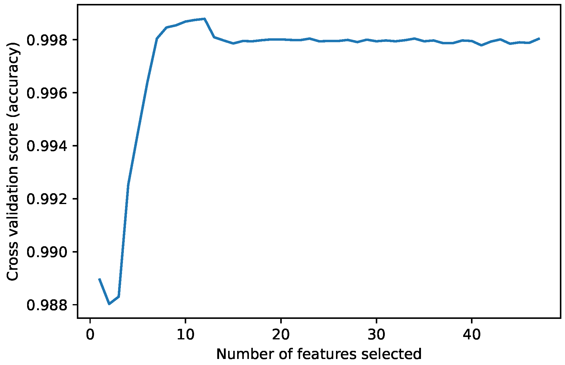
The Recursive Feature Elimination (RFE) function implements backwards selection of predictors based on predictor importance ranking. The predictors are ranked and, the least important ones are sequentially eliminated before modeling. The goal is to find a subset of predictors that can be used to produce an accurate model [42]. The model selected as the RFE estimator was a Decision Tree classifier with stratified k-fold cross-validation of five splits. After the algorithm selects the most important predictors, it performs an estimate of the accuracy obtained at different numbers of predictors used. As can be observed, in Figure 1, the best accuracy is achieved using 12 features. The features selected were: hour_cos, hour_sin, d_flow, ip.src_10.6.56.41, ClientId_131, ClientId_132, ClientId_133, ClientId_134, weekday_Friday, weekday_Saturday, weekday_Thursday, weekday_Wednesday.

In the network intrusion environment, it is common to find that one of the classes constitutes a very small minority of the data, where that minority represents the important cases to detect. When learning extremely unbalanced data, there is a significant probability that a selected sample contains few or even none of the minority class, resulting in an algorithm with poor performance for predicting the minority class [43]. This issue makes it easy to perform incorrect classifications in machine learning algorithms. Cross-validation (cv) is a statistical method of evaluating generalization performance that is more stable and thorough than using a split into a training and a test set. In cross-validation, the data are instead split repeatedly and multiple models are trained. The stratified k-fold cross-validation is a variation of k-fold that returns stratified folds. In stratified cross-validation, the folds are made by preserving the percentage of samples for each class, maintaining the data balancing relationship between classes. It is usually a good idea to use stratified k-fold cross-validation instead of k-fold cross-validation to evaluate a classifier, because it results in more reliable estimates of generalization performance [36].

Another approach that allows the minimization of data imbalance issue is the use of sampling techniques. SMOTE is a function to handle unbalanced classification problems. It performs a random down-sample to the majority class and, rather than over-sampling with replacement to the minority class, creating examples of synthetic minority classes to increase the minority class [43,44].

From the DAD dataset, there are 1088 anomalous and 96,894 normal packets. That means a 1:89 ratio, which shows an evident unbalanced data situation. To guarantee having taken samples from both classes the experimentation was performed by applying SMOTE inside a nested loop of Stratified k-fold cv with k = 5. By default, the SMOTE uses five k-neighbors. Initially, the minority class is over-sampled to about a 0.4 ratio. Then, the majority class is under-sampled to a 0.5 ratio, so each fold of the cross-validation split will have the same class distribution configured in SMOTE.

6. Models Training

For the experiments, all the models were evaluated within a nested stratified k-fold cv with an outer loop with a k = 5 and an inner loop also with k = 5, with SMOTE applied in the inner loop. In this section, the machine learning fitting techniques over the remaining data of the train k-fold cv set are exposed, computing Area Under the Receiver Operating Characteristic Curve (ROC AUC) from prediction scores. The results presented correspond to the average value of the inner cv.

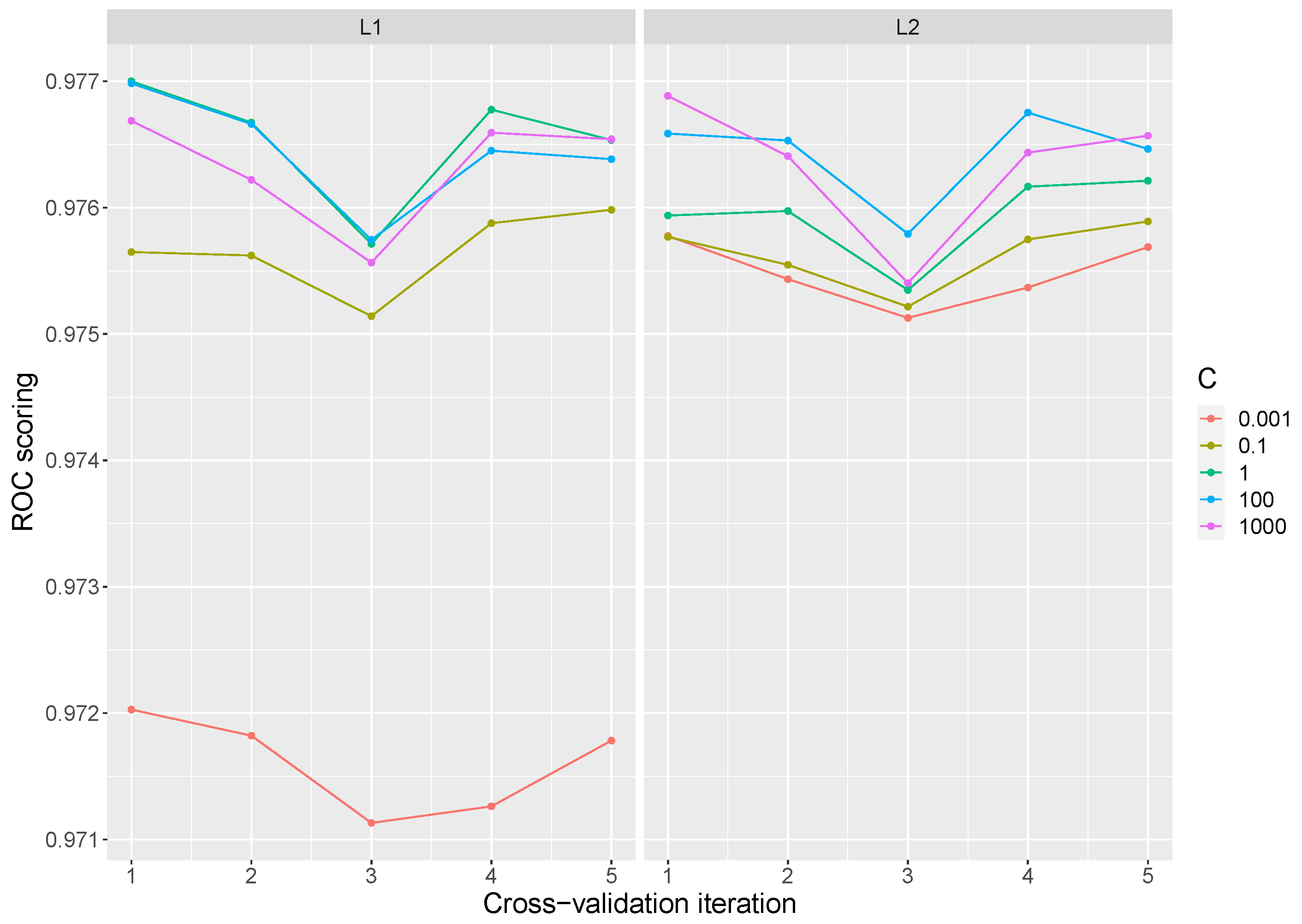
For Logistic Regression the liblinear solver was employed. A penalty of $L1$ and $L2$ were considered and the C parameter was adjusted to values of 0.001, 0.1, 1, 100, and 1000. Due to the stochastic nature of the algorithm, the results obtained vary depending on the iterations performed. The best result obtained has a value of 0.9790 with L2 penalty and a C value of 1000. The lowest value is 0.9676 with L1 penalty and a C value of 0.001. The global mean over all the iterations is 0.9756 with a standard deviation of $2.06\times {10}^{-3}$. Typically, large values of C give more freedom to the model, so a better performance is expected at high values of C. However, as can be seen in the Figure 2, the variation of the parameter C does not significantly improve the performance of the model with a suitable choice of penalty.

Table 1. Best Logistic Regression model by iteration.

CV	C	Penalty	Mean	Std. Deviation
1	1	l1	0.9770	$1.71\times {10}^{-3}$
2	1	l1	0.9767	$1.21\times {10}^{-3}$
3	100	l2	0.9758	$9.23\times {10}^{-4}$
4	1	l1	0.9768	$1.24\times {10}^{-3}$
5	1000	l2	0.9766	$1.87\times {10}^{-3}$

presents the best parameters selected for the best mean score in each of the inner cv, as well as the standard deviation obtained. The tuned parameters that exhibited the best results, in most cases, are C equal to 1 and an L1 penalty. The parameters performed in the table are those selected for model evaluation in the test split.

Among the Naive Bayes models previously mentioned, the Bernoulli Naive Bayes was selected. To find an optimal combination of hyperparameters that minimizes a predefined loss function, the results were calculated by varying the $\alpha$ over 0.01, 0.1, 0.5, 1, and 10. The mean ROC AUC value presented over all iterations is 0.9654 with a standard deviation of $3.23\times {10}^{-3}$. The least best ROC AUC value is 0.9587 with an $\alpha$ of 0.1, while the best is 0.9721 with $\alpha$ equal to 0.01. Figure 3 shows the mean by iteration of the results obtained in the hyperparameter tuning. As logistic regression, Bernoulli Naive Bayes does not improve the performance proportional to $\alpha$ values in each iteration.

Table 2. Best Naive Bayes model by iteration.

CV	$\mathit{\alpha }$	Mean	Std. Deviation
1	0.01	0.9663	$3.45\times {10}^{-3}$
2	0.01	0.9653	$2.69\times {10}^{-3}$
3	1.0	0.9668	$1.42\times {10}^{-3}$
4	10.0	0.9651	$3.23\times {10}^{-3}$
5	1.0	0.9650	$3.86\times {10}^{-3}$

presents the parameters that offer a better score in each inner iteration. These parameters will be used in the evaluation of the model. The best value obtained was 0.9721 with an $\alpha$ of 1 and a lowest standard deviation of $3.22\times {10}^{-3}$.

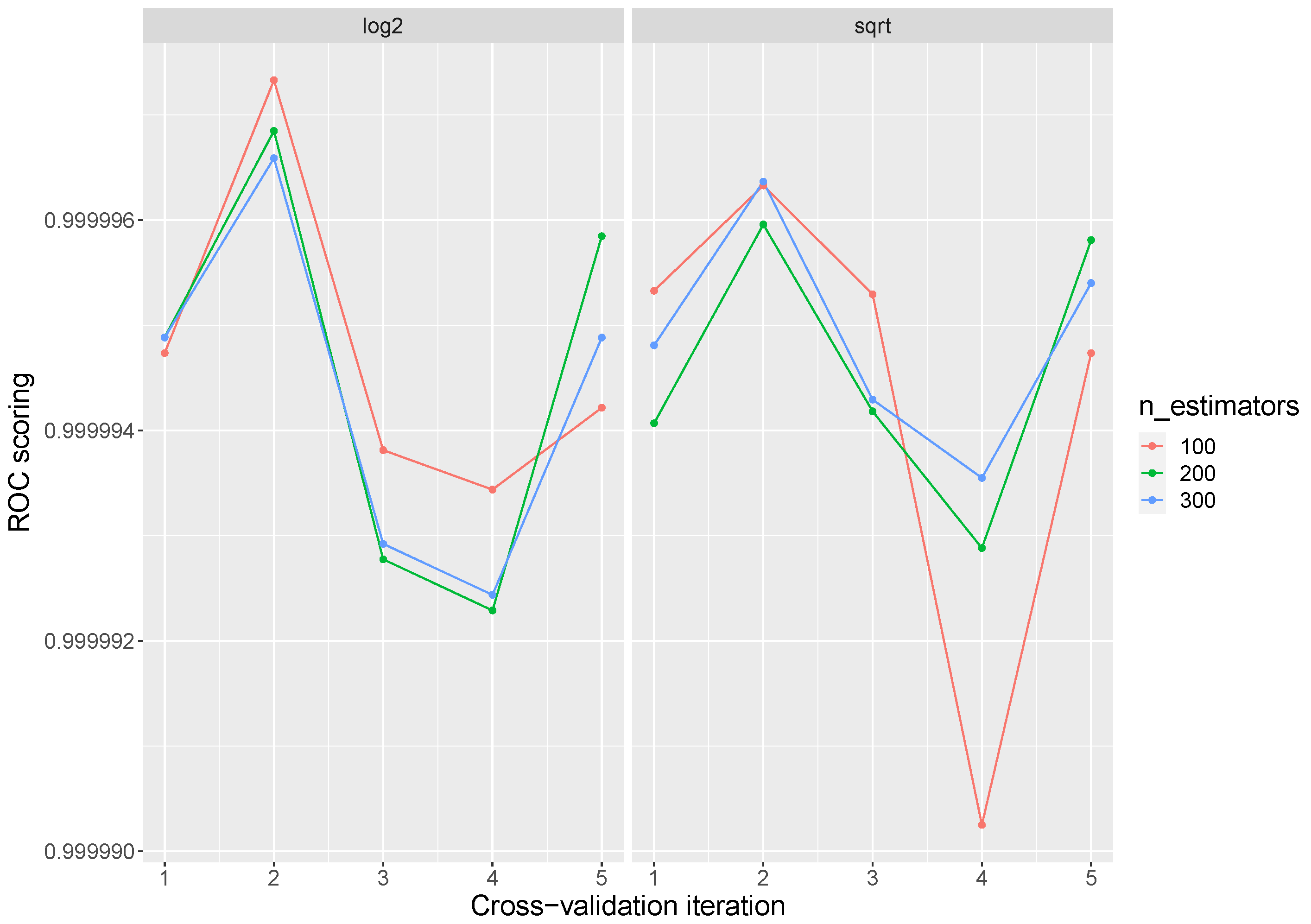
For Random Forest hyperparameter tuning, the most important settings are the number of trees in the forest (n_estimators) and the number of features considered for splitting at each leaf node (max_features). During the execution, the evaluation was tested with 100, 200, and 300 trees, and the $sqrt$ and $log2$ as max_features. The global average obtained was 0.9999 with a standard deviation of $5.57\times {10}^{-6}$ reaching a 1 ROC AUC in all the parameter combinations in some iteration. Figure 4 presents the average AUC ROC results by iteration. High points in the graph mean some 1 values in the iteration. Random Forest presents the best performance in the training stage.

Table 3. Best Random Forest model by iteration.

CV	Max_Features	n_Estimators	Mean	Std. Deviation
1	sqrt	100	1	$3.75\times {10}^{-6}$
2	log2	100	1	$9.78\times {10}^{-7}$
3	sqrt	100	1	$3.03\times {10}^{-6}$
4	sqrt	300	0.99	$6.30\times {10}^{-6}$
5	log2	200	1	$6.21\times {10}^{-6}$

shows the best parameters over each inner iteration. There are several parameterizations that obtain the best response over all the iterations. However, the number of trees and features can affect the time and performance of the model during its execution.

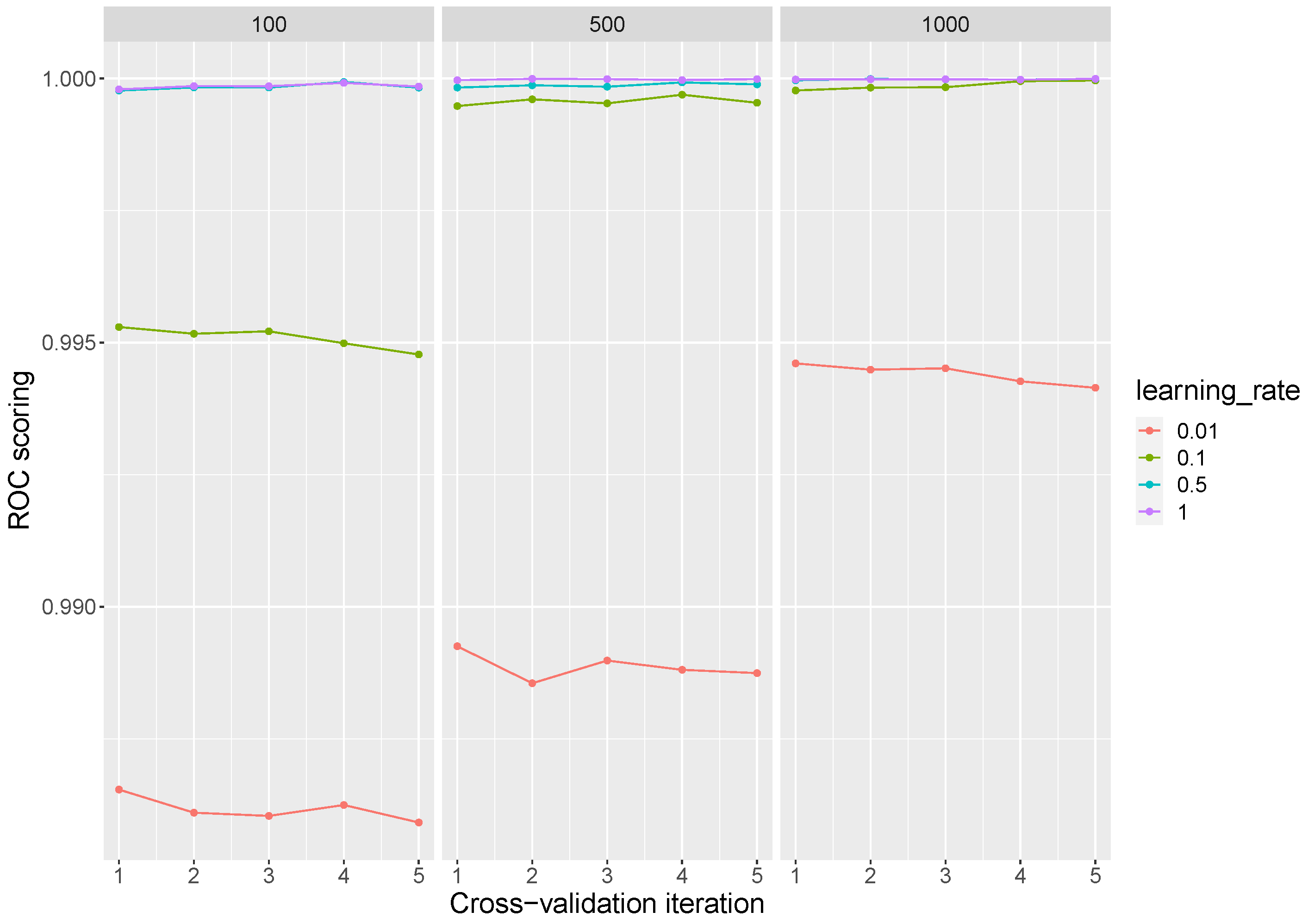
The AdaBoost classifier by default uses a Decision Tree classifier as a base estimator, initialized with max_depth = 1. To fit a good model it may be desirable to increase the number of trees of the classifier, although this may affect the performance of the system. For this model, the number of estimators used were 500, 1000, and 2000, and the learning rate values were 0.001, 0.01, and 0.1. The global AUC ROC average obtained was 0.9969 with a standard deviation of $1.69\times {10}^{-3}$.

In Figure 5, we can see how the increase of the learning rate parameter increases the performance of the model about the number of trees selected; even so, excellent results can be achieved with medium levels of learning rate at a low number of trees in the classifier.

Table 4. Best AdaBoost model by iteration.

CV	Learning_Rate	n_Estimators	Mean	Std. Deviation
1	1	1000	0.99998	$2.64\times {10}^{-5}$
2	1	500	1	$6.21\times {10}^{-6}$
3	1	500	0.99998	$8.24\times {10}^{-6}$
4	0.5	1000	0.99997	$2.10\times {10}^{-5}$
5	1	1000	1	$1.13\times {10}^{-5}$

shows the parameters that reach the highest average over the inner cross-validation implementation. With very low standard deviations values, and reaching scores of 1 in some iterations, the best models are found with high learning rate values and a large number of trees.

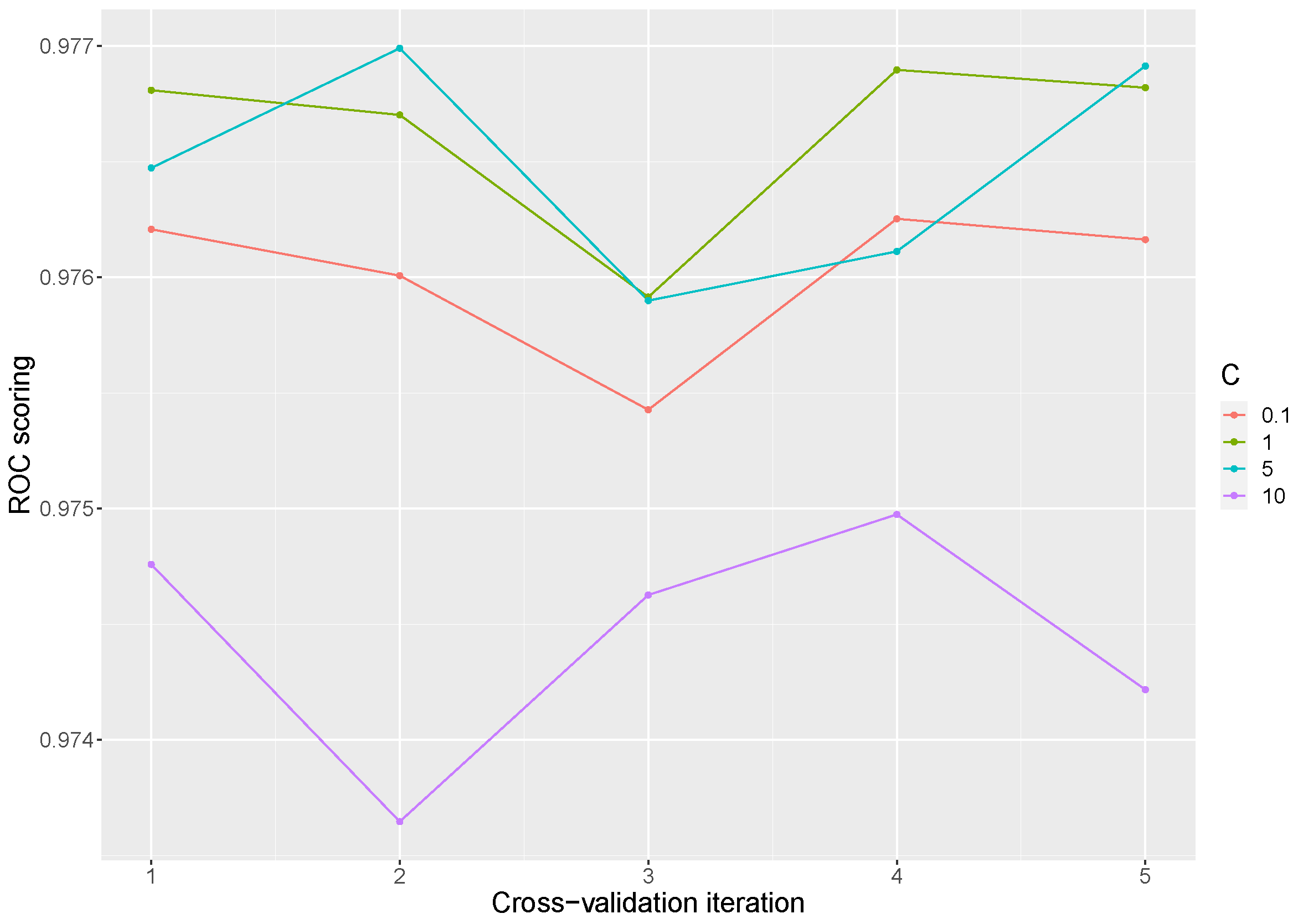
Finally, for Support Vector Machine, the linear vector classifier was adopted because it has more flexibility in the choice of penalties and loss functions and it should scale better to large numbers of samples. To improve the model accuracy, the C parameter was tuned. The C penalty parameter controls the trade-off between decision boundary and misclassification term, being fixed to 0.1, 1, 5, and 10. Taking into account all the experiments, an ROC AUC mean score of 0.9759 was reached, with a standard deviation of $1.74\times {10}^{-3}$.

Figure 6 shows the mean scoring obtained across the iterations, exhibiting the detriment of the model in a value of C equal to 10. The best means scores of the model are found at values of C of 1 and 5 as can be seen in

Table 5. Best SVM model by iteration.

CV	C	Mean	Std. Deviation
1	1	0.9768	$1.56\times {10}^{-3}$
2	5	0.9770	$1.39\times {10}^{-3}$
3	1	0.9759	$9.59\times {10}^{-4}$
4	1	0.9769	$1.23\times {10}^{-3}$
5	5	0.9769	$1.98\times {10}^{-3}$

.

7. Results and Models Comparison

To make predictions on data, it is necessary to use the data not managed to train the model. The performance estimate of the machine learning model is approved on the cross-validation test-split set. This section presents the results of the four traditional metrics: accuracy, precision, recall, and F1 for all the shallow machine learning models evaluated. Additionally, a comparison between the performance of the algorithms is made.

Figure 7a shows the mean accuracy values in each of the models over all of the iterations performed. Here, we can see how the lowest performance for this metric is presented by the Naive Bayes classifier. Models based on Decision Trees present the best results, obtaining values very close to the optimal result. In precision, again, the classifiers based on Decision Trees reach values of one in three of the five iterations performed, as illustrated in Figure 7b. For recall, in Figure 7c the best results are obtained by NB, with AdaBoost and RF having equally very satisfactory results. On the other hand, for the F1 metric, (Figure 7d) AdaBoost and RF, again, are the classifiers that achieve the best results in all iterations, reaching outstanding results compared to the rest of the classifiers.

Table 6. Best score model by iteration.

Score	NB	AdaBoost	LR	RF	Linear SVC
mean accuracy	0.8486	0.9998	0.9658	0.9998	0.9639
mean precision	0.0684	0.9954	0.1548	0.9919	0.1962
mean recall	1	0.9917	0.4659	0.9954	0.7289
mean F1	0.1279	0.9935	0.2323	0.9935	0.3090
std accuracy	$1.68\times {10}^{-3}$	$5.59\times {10}^{-5}$	$1.12\times {10}^{-3}$	$1.27\times {10}^{-4}$	$2.15\times {10}^{-3}$
std precision	$7.47\times {10}^{-4}$	$5.54\times {10}^{-3}$	$8.35\times {10}^{-3}$	$1.07\times {10}^{-2}$	$1.91\times {10}^{-2}$
std recall	0	$5.99\times {10}^{-3}$	$4.57\times {10}^{-2}$	$5.65\times {10}^{-3}$	$9.09\times {10}^{-2}$
std F1	$1.31\times {10}^{-3}$	$2.53\times {10}^{-3}$	$1.45\times {10}^{-2}$	$5.64\times {10}^{-3}$	$3.08\times {10}^{-2}$

presents the means to all iterations of all classifiers together with their standard deviation. The Naive Bayes classifier has the lowest accuracy values among all the models, but it is the only one to obtain a perfect recall. As expected, due to the similarity in the construction of the models, the LR and SVM classifiers offer very similar results. Both classifiers have an accuracy of 0.96 and a precision of around 0.1 and an F1 of 0.3.

These results confirm the tree-based classifiers as the best classifiers for this dataset, reaching almost perfect values (close to 1.0) and, also presenting the lowest standard deviations, guaranteeing stability in the classifier.

8. Conclusions and Future Work

In order to mitigate traffic anomalies, developers need to enhance new techniques for detecting affected IoT devices. Machine Learning techniques have recently gained credibility in a successful application for the detection of network anomalies including IoT networks. Given the scarcity of IoT datasets, the DAD emerged as a mechanism to know the behavior of dedicated, lightweight devices in IoT-MQTT networks. The DAD is a complete and labeled dataset with previous analysis and is intended to be applied to detect traffic anomalies using ML algorithms. Then, this work aims to demonstrate that the DAD dataset can be used to detect anomalies in MQTT-IoT traffic networks.

To do so, the data must be conditioned to be perfectly understandable to the classifier. Data cleaning and conditioning routines attempt to smooth out noise while identifying outliers in the data. The use of cyclical characteristics creates unequivocal variables for the classifier, while the discretization techniques provide a high-order ranking of values that can smooth out the relationships between observations. The RFE algorithm was implemented, eliminating dependencies and collinearities between features, minimizing errors and computational efforts. To ensure the optimal performance of the models, the hyperparameters’ tuning was applied. This guarantees the appropriate values to avoid overfitting. Besides, the use of SMOTE, in conjunction with stratified k-fold cross-validation as a data management technique for unbalanced data, allowed us to solve the evident presence of a minority class in the dataset, in a simple way that substantially improves the performance of the classifier.

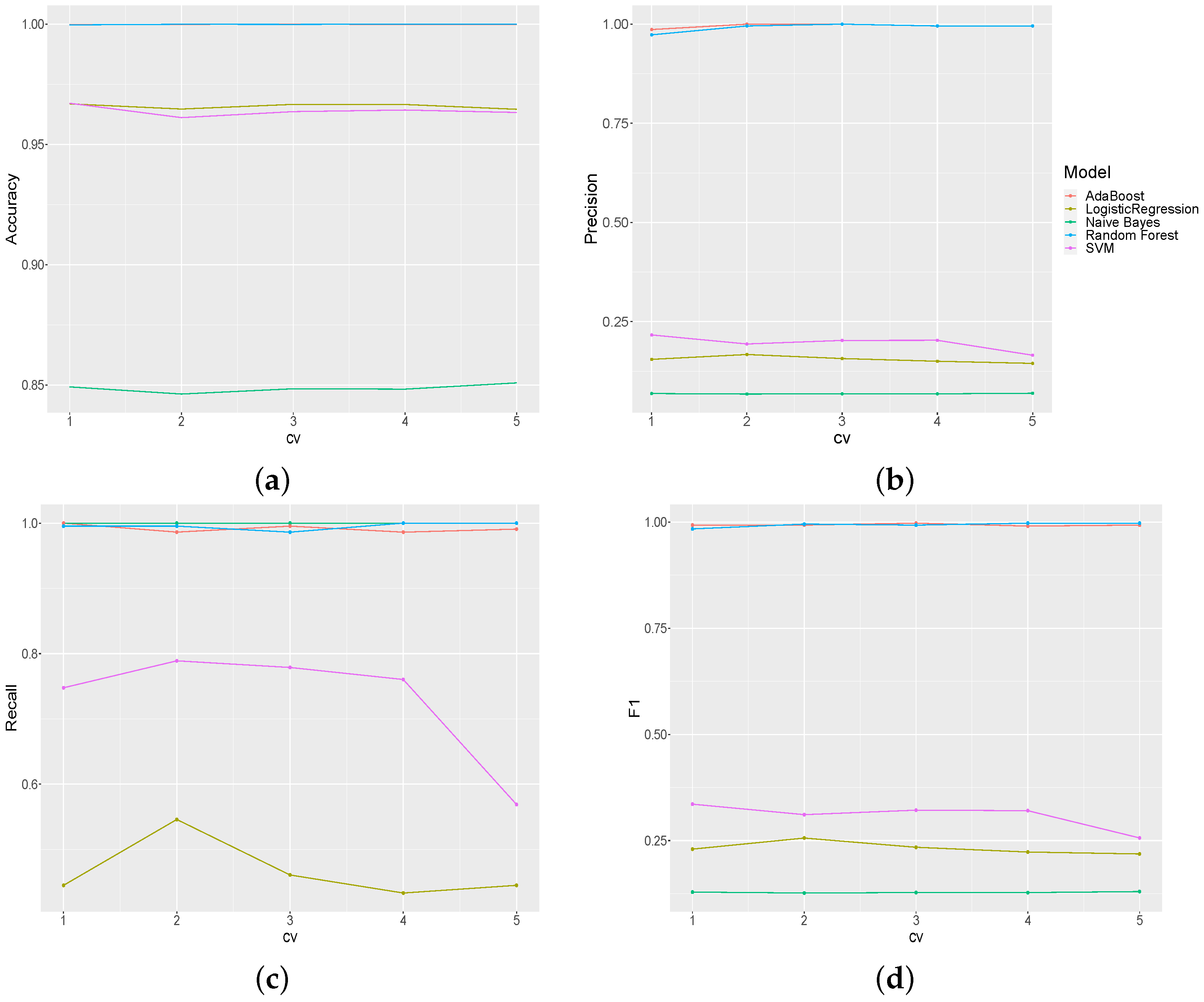
With respect to the techniques, We have selected five widely used shallow machine learning algorithms, such as Logistic Regression, Naive Bayes, Random Forest and Linear Support Vector Machine. Three of them base their behavior on statistical linear functions, Logistic Regression, Naive Bayes, and SVM. As expected, they obtain very similar results. On the other hand, the tree-based classifiers, RF and Adaboost, behave similarly.

During the training stage, all the models behave exceptionally, where the lowest score presented is from the Naive Bayes classifier with a mean ROC AUC of 0.9587 and the highest reached by an RF and Adaboost with the value of 1.

In the test stage, the results obtained by the tree-based classifiers present excellent traditional metric values, providing a notable performance of their applications in the realm of behavior-based Intrusion Detection Systems and exhibiting a substantial improvement efficiency, providing low error rates and noise resistance.

The DAD dataset was created to be used for the detection of anomalies in MQTT-IoT traffic networks. Hence, these experiments confirm that the dataset can be used for the application of traffic anomaly detection in IoT, applying optimization techniques.

Due to the novelty of this dataset, there are still no other works conducted on it. As a result, we present the first application of ML algorithms on it for anomaly detection in IoT networks. Future work could include the application of other types of Machine Learning algorithms to the dataset, comparing the results obtained, to verify the effectiveness of the exposed classifiers.