A Novel Opposition-Based Arithmetic Optimization Algorithm for Parameter Extraction of PEM Fuel Cell

Abstract

The model-identification and parameter extraction are a well-defined method for modeling and development purposes of a proton exchange membrane fuel cell (PEMFC) to improve the performance. This paper introduces a novel opposition-based arithmetic optimization algorithm (OBAOA) for identifying the unspecified parameters of PEMFCs. The cost function is defined as the sum of the square deviations between the experimentally measured values and the optimal achieved values from the algorithm. Ballard Mark V PEM fuel cell is employed and analyzed to demonstrate the capability of the proposed algorithm. To demonstrate system efficiency, simulation results are compared to those of other optimizers under the same conditions. Furthermore, the proposed algorithm is validated through benchmark functions. The final results revealed that the proposed opposition-based arithmetic optimization algorithm can accurately retrieve the parameters of a PEMFC model.

1. Introduction

The demand for clean energy has kept increasing in recent years due to global warming and depleting oil reserves [1,2]. Fuel cells have drawn significant attention in recent years due to high efficiency and no emission of greenhouse gases. In recent years, fuel cell research has grown significantly due to possible applications such as stationary power generation and automotive applications [3]. PEMFCs have particularly drawn attention for transport applications. It has many advantages such as low operating temperature, short start-up and shut-down time, high efficiency, no waste is generated as the by-product is water [4,5]. Due to compact size, low operating temperature, and quick start-up time makes PEMFCs a reliable candidate for medium power applications like smart grid, micro gird, and power electronic devices [6]. The fuel cell has three main components: anode, cathode, and electrolyte. Both anode and cathode contain a layer of catalyst, which is separated by an electrolyte membrane to perform the redox reaction. However, the voltage (1.0 V) and current density (500–1000 mA/cm²) delivered by a single cell is too low for any practical application, so a number of stacks are connected in series to deliver sufficient power for practical application. The performance of a fuel cell depends on multiple parameters such as operating temperature, inlet pressure of fuel and reactant, and conductivity of the membrane. In order to utilize fuel cell for wide range of application evaluation of performance under various operating conditions is necessary. Moreover, development of a mathematical model to simulate the dynamic variation in operating conditions and fuel cell performance is necessary for its integration in smart grid/microgrid [7].

Both theoretical and experimental studies have been performed to optimize the factors affecting performance such as pressure, temperature, flow rate of fuel and oxidant, reaction kinetics, and membrane thickness to get the maximum power density from fuel cell [8]. As the fuel cell performance depends on multiple interdependent factors, which makes it really difficult to develop a mathematical model to evaluate the multivariable, complex, and interrelated parameters affecting the fuel cell performance [9]. In recent years, remarkable research and development has been performed to get a better understanding of the function of PEMFC characteristics via mathematical modeling. The modeling achieves great significance in the outlook of simulation, design, exploration, and progress of high-efficiency fuel cell systems [10,11,12]. A reliable model facilitates monitoring of fuel cell behavior for process monitoring and designing a suitable power conditioning unit for various power applications. The development of a precise parameter estimation method using the experimental data is a pre-requisite to develop a mathematical model of fuel cell and design an appropriate power control algorithm [13]. Two different approaches have been utilized to develop a mathematical model of the fuel cell systems. In the first approach, a mechanistic model is built to simulate the heat, mass transfer, reaction kinetics, membrane conductivity, and crossover of reactants through the electrolyte membrane encountered in fuel cells [14,15]. In this approach, a three-dimensional multiphase model of fuel cell system is developed, in which the gas and liquid two-phase flow in channel and porous electrodes are investigated in detail. This approach of precise estimation of model parameters is hindered by the nonlinear and complex relations of the electrochemical equations. In the second approach, a mathematical model is developed on the basis of empirical or semi-empirical equations, which are utilized to predict the effect of different input parameters on the voltage–current characteristics of the fuel cell, without examining the physical and electrochemical phenomena taking place in fuel cell system [16]. The electrical equivalent models of fuel cell are mainly divided into static and dynamic models. The static models depends on steady-state operation of fuel cell based on polarization curve [17,18] and the dynamic models rely on characteristics of electrical terminal represented by a set of passive elements [19,20]. Although mechanistic models have been developed to evaluate the optimum parameters to get the maximum output from the fuel cell system, the actual performance of fuel cell observed in experimental studies is not precisely the same as observed in theoretical studies, irrespective of models, because of assumptions and approximations are made in modelling [21]. In order to develop the precision of the models and make it reflect the actual fuel-cell performance, it is essential to improve the parameters of the models. However, a little effort has been put forward in the area of parameters optimization.

Generally, the statistics contained in any PEMFC datasheet are insufficient to determine the effective set of parameters. However, if the precise parameters are not specified, there are significant variations between the data obtained from the model and that listed in the manufacturer’s datasheet. PEMFC parameter identification can be approached as an optimization challenge, and a variety of meta-heuristic techniques can be implemented to find the best solution. Over the last ten years, various meta-heuristic optimization techniques have been applied to address the issue of PEMFC parameter estimation, which utilizes two important search strategies: (a) exploration/diversification and (b) exploitation/intensification [22,23]. The first method explores the search space globally, which avoids local optima and resolving local optima entrapment, whereas the second method explores the nearby promising solutions to improve their quality locally [24]. A proper balance between these two strategies is required to get the optimum performance. The classification of meta-heuristics method is based in the evolutionary algorithms, swarm intelligence algorithms, physics-based methods, and human-based methods. However, there is no single optimized algorithm, which can solve all optimization problems. Most of the researchers either modify an existing algorithm or propose a new algorithm to get better result [25]. Different meta-heuristic algorithms have been utilized for parameter optimization of PEMFCs such as particle swarm optimization (PSO) [26], genetic algorithm (GA) [27], artificial neural network (ANN) [28], differential evolution (DE) [29], artificial immune system (AIS) [30], artificial bee colony (ABC) [31], bird mating optimization (BMO) [32], biography-based optimization (BMO) [33], seeker optimization algorithm (SOA) [34], backtracking search algorithm (BSA) [35], improved teaching learning-based optimization (ITLBO) [36]. Slime mold algorithm (SMA) [37], moth-flame optimization (MFO) [38], Archimedes optimization algorithm [39], Jellyfish search algorithm (JSA) [40], bonobo optimizer [41], and hybrid GWO algorithm [42] have been implemented to identify the unknown parameters of PEMFC. In this article, the authors have proposed an improved opposition-based arithmetic optimization algorithm for parameter extraction of PEMFC. To the best of the authors’ knowledge, arithmetic optimization algorithm (AOA) has not been explored in this field, therefore, in this article authors have examined the performance of improved AOA for parameter extraction of fuel cells.

The main contribution of this research paper is as follows:

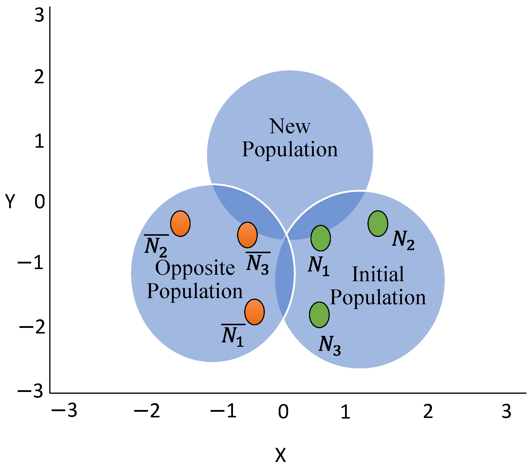
• An improved arithmetic optimization algorithm (AOA) algorithm is formulated that employs the opposition-based learning method for population initialization, preventing the accumulation of too many solutions in one location and resulting in a more efficient global search.
• The performance of the proposed algorithm is evaluated on ten benchmark functions and experimental results clearly depicts that the OBAOA is very efficient and accurate.
• The performance of proposed OBAOA algorithm is further accessed for parameter extraction of Ballard Mark V PEFMC.

The manuscript is organized as follows: Section 2 describes the theoretical and mathematical model of the PEMFC, Section 3 includes the formulation of OAOA technique. Section 4 discusses the results and findings. Finally, Section 5 provides the overall conclusive remarks of the proposed study.

2. Theory and Modeling of Proton Exchange Membrane Fuel Cell

There are three main components of a fuel cell: anode, cathode, and electrolyte. The fuel oxidation and oxygen reduction take place at anode and cathode, respectively. An electrolyte membrane separates the anode and cathode and allows conduction of protons to complete the electric circuit. The oxidation and reduction reaction are shown by Equations (1) and (2), respectively. The overall reaction is represented by Equation (3) [43,44].

Oxidation: 2H₂ → 4H⁺ + 4e⁻

(1)

Reduction: O₂ + 4H⁺ + 4e⁻ → 2H₂O

(2)

Complete reaction: 2H₂ + O₂ → 2H₂O

(3)

At open circuit potential the cell voltage can be expressed by Equation (4):

$$V_{\mathrm{Cell}}^{\mathrm{OCV}}=E_{{\mathrm{O}}_2/{\mathrm{H}}_2\mathrm{O}}^r-E_{{\mathrm{H}}_2/{\mathrm{H}}^{+}}^r$$

(4)

At standard conditions (1.0 atm pressure and 25 °C), the fuel cell open circuit voltage (OCV) should be 1.229 V. However, the measured OCV at room temperature is around 1.0 V, due to the losses associated with the fuel cell. The cell voltage ($V_{\mathrm{cell}}$) is expressed by Equation (5) when the current ($I_{\mathrm{cell}}$) is drawn from the cell.

$$V_{\mathrm{cell}}=E_{\mathrm{Nernst}}-V_{\mathrm{activation}}-V_{\mathrm{concentration}}-V_{\mathrm{ohmic}}$$

(5)

$$E_{\mathrm{Nernst}}=1.229–0.85\times {10}^{-4}\left(T–298.15\right)+4.3085\times {10}^{-5}T \left[ln \left(P_{{\mathrm{H}}_2}\right)+0.5 ln \left(P_{{\mathrm{O}}_2}\right)\right]$$

(6)

The activation overpotential of anode and cathode can be expressed as:

$$V_{\mathrm{activation}}=-\left[{\xi }_1+{\xi }_2+{\xi }_3\times T\times ln\left(C_{{\mathrm{O}}_2}\right)+{\xi }_4 ln\left(i\right)\right]$$

(7)

where $V_{\mathrm{activation}}$ is the voltage drop due to the activation of redox processing the anode and cathode. The ${\xi }_{\mathrm{n}}$ represents the parametric coefficients for each cell model, whose values are defined based on theoretical equations with kinetic, thermodynamic, and electrochemical foundations (Mann et al., 2000). The oxygen concentration at the catalyst layer of the cathode ($C_{{\mathrm{O}}_2}$, mol/cm³) is given by:

$$C_{{\mathrm{O}}_2}=\frac{P_{{\mathrm{O}}_2}}{5.08\times {10}^6\times e^{\frac{498}{T}}}$$

(8)

The mass transport affects the concentrations of hydrogen and oxygen at the anode and cathode, which affects the partial pressures of gases. The change in partial pressure of fuel and reductant rely on the electrical current and on the physical features of the system. The voltage drop due to concentration polarization is represented as:

$$V_{\mathrm{concentration}}=-b ln\left(1-\frac{i}{i_{max}}\right)$$

(9)

where $b$ is a parametric coefficient (V) that depends on the cell and its operation state, and $i$ represents the actual current density of the cell (A/cm²).

The ohmic drop ($V_{\mathrm{Ohmic}}$) in Equation (5) is represented as:

$$V_{\mathrm{Ohmic}}=i \left(R_M+R_c\right)$$

(10)

$$R_M={\rho }_M\frac{l}{A}$$

(11)

where $R_M$ is the resistance to the transfer of protons through the membrane (Ω), $R_c$ is the charge transfer resistance, ${\rho }_M$ is the specific resistivity of the membrane for the electron flow (Ω-m), $A$ is the active area of the cell (cm²) and $l$ is the thickness of the membrane, which separate electrodes. The following numerical expression for the resistivity of the Nafion membrane is used:

$${\rho }_M=\frac{181.6\times \left[1+0.03{\left(\frac{i_{FC}}{A}\right)}^{ }+0.062{\left(\frac{T}{303}\right)}^2{\left(\frac{i_{FC}}{A}\right)}^{2.5}\right]}{\left[\lambda -0.634-3\left(\frac{i_{FA}}{A}\right)exp\left(4.18\left(\frac{T-303}{T}\right)\right)\right]}$$

(12)

where 181.6/(λ − 0.634) is the specific resistivity (Ω-cm) at OCV at 30 °C, the exponential term in the denominator is the temperature factor correction if the cell is operating at different temperature. The parameter $\lambda$ is an adjustable parameter with a maximum value of 24. This parameter is influenced by the preparation procedure of the membrane and is a function of relative humidity and stoichiometry relation of the anode gas.

If ‘$n$’ number of stacks are combined then the cell voltage is defined as:

$$V_{\mathrm{cell}}=n\times \left(E_{\mathrm{Nernst}}-V_{\mathrm{activation}}-V_{\mathrm{concentration}}-V_{\mathrm{ohmic}}\right)$$

(13)

At a given temperature ($T$), the partial pressure of fuel ($P_{{\mathrm{H}}_2}$) and oxidant ($P_{{\mathrm{O}}_2}$) is given by following equations:

$$P_{{\mathrm{H}}_2}=\frac{0.79}{0.21}{P}_{{\mathrm{O}}_2}$$

(14)

$$P_{{\mathrm{O}}_2}=P_c-R{H}_c{P}_{{\mathrm{H}}_2\mathrm{O}}^{*}-P_{{\mathrm{N}}_2}\exp \left(\frac{0.291\frac{i}{A}}{T^{0.832}}\right)$$

(15)

If ${\mathrm{H}}_2$ and ${\mathrm{O}}_2$ are used as reactant then the partial pressure of oxygen and hydrogen is given as:

$$P_{{\mathrm{O}}_2}=R{H}_c{P}_{{\mathrm{H}}_2\mathrm{O}}^{*}\left[{\left(\frac{\exp \left(\frac{4.192\left(\frac{i}{A}\right)}{T^{1.334}}\right)\left(R{H}_c{P}_{{\mathrm{H}}_2\mathrm{O}}^{*}\right)}{P_c}\right)}^{-1}-1\right]$$

(16)

$$P_{{\mathrm{H}}_2}=R{H}_a{P}_{{\mathrm{H}}_2\mathrm{O}}^{*}\left[{\left(\frac{\exp \left(\frac{1.635\left(\frac{i}{A}\right)}{T^{1.334}}\right)\left(R{H}_a{P}_{{\mathrm{H}}_2\mathrm{O}}^{*}\right)}{P_a}\right)}^{-1}-1\right]$$

(17)

where $R{H}_c$ and $R{H}_a$ are relative humidity at the cathode and anode, respectively. $P_c$ and $P_a$ are the inlet pressure at cathode and anode, respectively. The $P_{{\mathrm{N}}_2}$ is partial pressure of nitrogen at the cathode. The $P_{{\mathrm{H}}_2\mathrm{O}}^{*}$ is saturated vapor pressure (atm), which is calculated as:

$$lo{g}_{10}\left(P_{{\mathrm{H}}_2\mathrm{O}}^{*}\right)=2.95\times {10}^{-2}\left(T–273.15\right)–9.18\times {10}^{-5}{\left(T–273.15\right)}^2+1.44\times {10}^{-7}{\left(T–273.15\right)}^3–2.18$$

(18)

Formulation of Objective Function

In this research work, sum of squared error (SSE) is adopted as an optimization function (OF) for the identification of unknown parameters (${\zeta }_1$, ${\zeta }_2$, ${\zeta }_3$, ${\zeta }_4$, $\lambda$, $R_c$, and $b$) of PEMFC, which is generally used by the authors in the existing literature [45,46,47]. The objective function is defined as follows:

$$\mathrm{OF}=\mathrm{Minimize}\left(SSE\right)=\mathrm{Minimize}\left({\displaystyle \sum }_{i=1}^N{\left[V_{\mathrm{measured}}\left(i\right)-V_{\mathrm{estimated}}\left(i\right)\right]}^2 \right)$$

(19)

where $N$ represents the number of measured values, $i$ denotes the number of iterations, $V_{\mathrm{measured}}$ denotes the measured voltage while $V_{\mathrm{estimated}}$ denotes the estimated value of voltage for PEMFC.

3. Optimization Method

3.1. Conventional Arithmetic Optimization Algorithm

Arithmetic optimization algorithm (AOA) is a stochastic population-based metaheuristic optimization algorithm proposed by Abualigah et al. [48] in the year 2021. The algorithm is motivated by the distribution behavior of four key arithmetic operators in the field of mathematics, which includes addition, subtraction, multiplication, and division. In the area of science and engineering, there are complex, non-convex, and high dimension problems, which are difficult to solve using conventional gradient-based optimization algorithms. Metaheuristic is a high-level search algorithm that easily finds the optimal solution for diverse problems without getting stuck in local optimal solution. These algorithms first create a random solution in the search space and iteratively discovers the solution through different search strategies. The phenomenon of how these algorithms update its solution is defined by mathematical behavior of algorithms. Based on these mathematical-concepts, these algorithms are classified as evolutionary, swarm, physics-based, and human-based algorithms. Genetic algorithm (GA), particle swarm optimization (PSO), gravitational search algorithm (GSA), whale optimization algorithm (WOA), and grey wolf optimization (GWO) are some of the metaheuristic algorithms that have efficiently solved non-linear and high-computational engineering design problems. Exploration and exploitation are other unique characteristics that define the functionality of these algorithms. Exploration is defined as the global search capability of the algorithm, while exploitation is defined as the capability of algorithm to explore the nearby promising regions. The efficiency of a metaheuristic algorithm depends on how efficiently the algorithm maintains the balance between exploration and exploitation. AOA uses high and low dispersion nature of arithmetic operators to creates this balance. Multiplication and division operators have high distributed values, therefore these operators are used in the exploration phase to discover the optimal solution in a diverse region of search space with the following equations:

$$x_{i,j}\left(C_{\mathrm{Iter}}+1\right)=\{\begin{array}{c}best\left(x_j\right)÷\left(MOP+ϵ\right)\times \left(\left(U{B}_j-L{B}_j\right)\times \mu +L{B}_j\right), r_2<0.5\\ best\left(x_j\right)\times MOP\times \left(\left(U{B}_j-L{B}_j\right)\times \mu +L{B}_j\right), \mathrm{otherwise}\end{array}$$

(20)

where $x_{i,j}$ represents the jth position of the ith solution, $best\left(x_j\right)$ is the jth position of the best obtained solution, $U{B}_j$ and $L{B}_j$ are the upper and the lower bound of the jth position, $ϵ$ is a constant parameter, $\mu$ is the control parameter that regulates the search process, and $r_2$ is the random number in the range [0, 1]. The MOP is math optimizer probability and defined as:

$$MOP\left(C_{\mathrm{Iter}}\right)=1-\frac{{(C_{\mathrm{Iter}})}^{\raisebox{1ex}{$1$}\!\left/ \!\raisebox{-1ex}{$\alpha $}\right.}}{{(M_{\mathrm{Iter}})}^{\raisebox{1ex}{$1$}\!\left/ \!\raisebox{-1ex}{$\alpha $}\right.}}$$

(21)

where $C_{\mathrm{Iter}}$ represents the current iteration, $M_{\mathrm{Iter}}$ represents the maximum number of iterations, and $\alpha$ is the constant parameter.

Subtraction and multiplication operators have low distributed values, therefore, these operators easily find the optimal solution in the areas that were discovered in the exploration phase. These exploitation operators iteratively reach the solution with the following equations:

$$x_{i,j}\left(C_{\mathrm{Iter}}+1\right)=\{\begin{array}{c}best\left(x_j\right)-\left(MOP+ϵ\right)\times \left(\left(U{B}_j-L{B}_j\right)\times \mu +L{B}_j\right), r_3<0.5\\ best\left(x_j\right)+MOP\times \left(\left(U{B}_j-L{B}_j\right)\times \mu +L{B}_j\right), \mathrm{otherwise}\end{array}$$

(22)

where $r_3$ is the random number defined in range [0, 1].

The exploration and exploitation phases are balanced by Math Optimizer accelerated (MOA) function, which is defined as:

$$MOA\left(C_{\mathrm{Iter}}\right)=Min+C_{\mathrm{Iter}}\times \left(\frac{Max-Min}{M_{\mathrm{Iter}}}\right)$$

(23)

where min and max represent the minimum and the maximum value of the accelerated function. Exploration phase is executed when the value of $r_1$, which is a random number in range [0, 1] is greater than MOA, otherwise the exploitation phase is executed.

3.2. Opposition-Based Learning

In 2005, Tizhoosh et al. introduced the phenomenon of opposition-based learning (OBL) [49]. The basic principle of OBL is that it imitates the opposite relationship among agents. Over the last few years, artificial intelligence field has experienced tremendous growth and researchers are exploring and building innovative algorithms so as to enhance the performance of existing algorithms. OBL is one of the novel concepts that finds application in metaheuristic [50] and other artificial intelligence algorithms. OBL considers agents and their opposite counterpart in order to better explore the search space and find global optimal solution. Figure 1 shows the mechanism of OBL. The fundamental concept of OBL is outlined as follows:

Figure 1. Illustration of opposition-based learning mechanism [2].

Let $N$ be a real number in the search space [$k_L$, $k_U$], then its opposite counterpart is defined as follows:

$$\overrightarrow{N}=k_L+k_U-N$$

(24)

In the higher dimensional space, the $N$ is expressed as:

$N_k=$ [$N_{k_1}$, $N_{k_2}$, …, $N_{k_t}$] and defined in the search space [$k_{Lt}$, $k_{Ut}$],

where $t=$ 1, 2, 3, …, n. Then, the opposite points are defined as:

$${\overrightarrow{N}}_k=k_{Lt}+k_{Ut}-\left[{\overrightarrow{N}}_{k1},{\overrightarrow{N}}_{k2},\dots \dots \dots \dots \dots \dots {\overrightarrow{N}}_{kt}\right]$$

(25)

3.3. Proposed Algorithm

This section outlines the proposed opposition-based arithmetic optimization algorithm (OBAOA). In the field of optimization, local optima avoidance capability and convergence rate are two critical parameters, which define the performance of the algorithm. Most of the metaheuristic algorithms quickly converges and avoids local optimal solution. However, some algorithms fail to explore entire search space and get trapped in local optimal solution. In this area, researchers are exploring new ways such as modification of existing algorithm, hybridization of two or more algorithms to overcome these limitations.

AOA also has poor exploration capability and did not discover a global optimal solution and have slow rate of convergence. Thus, in this article, authors have enhanced the performance of AOA by incorporating the opposition mechanism and have proposed opposition OBAOA. OBL mechanism allows the algorithm to discover global optimal solution and improve convergence rate and thereby boost exploration capability of the algorithm. In OBAOA, the opposition-based principle is first incorporated in the initialization phase and later in the operational phase. The flow chart of OBAOA is shown in Figure 2 and the mathematical model is outlined as follows:

Figure 2. Flow chart of opposition-based arithmetic optimization algorithm.

Step 1

Initialization: Generate the random candidate solution in the defined space as:

$$X=\left[\begin{array}{ccc}{p}_{1,1}& \begin{array}{ccc}{p}_{1,2}& \dots & \dots \end{array}& p_{1,d}\\ p_{2,1}& \begin{array}{ccc}{p}_{2,2}& \dots & \dots \end{array}& p_{2,d}\\ p_{n,1}& \begin{array}{ccc}{p}_{n,2}& \dots & \dots \end{array}& p_{n,d}\end{array}\right]$$

(26)

where $n$ is the number of solution and $d$ is the dimension.

Step 2

Opposition Based Learning: Generate the opposite solution in the search space using Equation (25);

Step 3

(Initialize the constant parameters): Initialize the parameters α, μ and ϵ;

Step 4

(Fitness evaluation): Evaluate the fitness of opposite candidate solution;

Step 5

(Ranking): Sort the fitness and determine the best solution;

Step 6

(Evaluate constant and time varying parameters): Use Equations (21) and (23) to estimate the MOA function and MOP and generate random numbers $r_1$, $r_2$, $r_3$ in the range [0, 1];

Step 7

(AOA candidate solution position updating mechanism):

if $r_1>$ MOA;

update position of each candidate solution using the following mechanism.

• Implement exploration phase:

•         if $r_1>$ 0.5;
          update the position using multiplication model of Equation (20).
          Else;
          update the position using division model of Equation (20).
          Else;

• Implement exploitation phase:

•         if $r_3>$ 0.5;
          update the position using addition model of Equation (22).
          Else;
          update the position using subtraction model of Equation (22).

Step 8

(Monitor the positions of each candidate solution): Determine the opposite candidate solution that moves beyond the search space and reinitialize their position within the boundaries;

Step 9

(Termination criteria): If minimum error or maximum number of iterations is accomplished the algorithm ends. Otherwise repeat Steps (5) to (8);

Step 10

(Final result): The position of best candidate solution represents the global optimal solution.

4. Results and Discussion

In this section, a benchmark test research approach was used to evaluate the proposed algorithm in the case of parameter identification for PEMFC. Table 1 displays the ten benchmark test functions, one to seven of which are unimodal and the remaining functions are multimodal. Some well-known meta-heuristic algorithms, such as ant lion optimizer (ALO) [51], dragonfly algorithm (DA) [52], grasshopper optimization algorithm (GOA) [53], and multiverse optimization (MVO) [54] are especially compared to assess the precision and efficiency of the suggested algorithm. The statistical outcomes of benchmark test functions are shown in Table 2. In this research paper, the benchmark functions are denoted by the letter “F” accompanied by a number (e.g., F1).

Table 1. Benchmark functions.

ID	Mathematical Expression	Dim	Lower	Upper	Type
F1	$f_1\left(x\right)={\displaystyle \sum }_{i=1}^n{x}^2$	30	−100	100	Unimodal
F2	$f_2\left(x\right)={\displaystyle \sum }_{i=1}^n\left|x_i\right|+{\displaystyle \prod }_{i=1}^n\left|x\right|$	30	−10	10	Unimodal
F3	$f_3\left(x\right)={\displaystyle \sum }_{i=1}^n\left({\displaystyle \sum }_{j-1}^i{x}_j\right)$	30	−100	100	Unimodal
F4	$f_4\left(x\right)=ma{x}_i\left[\left|x\right|,1\le i\le n\right]$	30	−100	100	Unimodal
F5	${\displaystyle \sum }_{i=1}^{n-1}\left[100{(x_{i+1}-x_i^2)}^2+{(x_i-1)}^2\right]$	30	−30	30	Unimodal
F6	${\displaystyle \sum }_{i=1}^n{\left(\left|x_i+0.5\right|\right)}^2$	30	−100	100	Unimodal
F7	${\displaystyle \sum }_{i=1}^{n}i{x}_i^4+random\left[0, 1\right]$	30	−1.28	1.28	Unimodal
F8	${\displaystyle \sum }_{i=1}^n-x_i\sin \left(\sqrt{\left|x_i\right|}\right)$	30	−500	500	Multimodal
F9	${\displaystyle \sum }_{i=1}^n\left[x_i^2-10\cos \left(2\pi x_i\right)+10\right].n$	30	−5.12	5.12	Multimodal
F10	$-20\exp \left(-0.2\sqrt{\frac{1}{n}}{\displaystyle \sum }_{i=1}^n{x}_i^2\right)-\exp \left(\frac{1}{n}{\displaystyle \sum }_{i=1}^n\cos \left(2\pi x_i\right)\right)$ + 20 + e	30	−32	32	Multimodal

Table 2. Statistical results of benchmark test functions.

Algorithms		F1	F2	F3	F4	F5	F6	F7	F8	F9	F10
OBAOA	MEAN	1.54 × 10−122	0	4.05 × 10−112	3.81 × 10−125	2.88 × 10−17	6.8817 × 10−2	7.17 × 10−16	−1.4632 × 104	6 × 10−51	5.33 × 10−43
	SD	3.0876 × 10−32	0	1.099 × 10−18	0	2.71 × 10−3	5.4317 × 10−3	1.15 × 10−4	3.0044 × 10−2	1.63 × 10−4	1.82 × 10−11
ALO	MEAN	9.06 × 10−10	1.56 × 10−5	8.02 × 10−5	3.36 × 10−5	5.8065 × 10−3	4.3 × 10−9	4.7488 × 10−2	−2.1542 × 102	1.9899 × 10−3	1.63 × 10−5
	SD	7.9531 × 10−5	2.33 × 10−2	4.4256 × 10−4	2.647 × 10−3	4.1108 × 10−2	2.0335 × 10−3	7.6 × 10−1	2.1278 × 103	2.5977 × 10−1	2.001 × 10−2
DA	MEAN	1.2477 × 10−2	5.789 × 10−1	5.137 × 10−2	2.6485 × 10−3	1.5026 × 10−3	1.115 × 10−2	8.381 × 10−3	−2.3522 × 103	1.8527 × 10−1	2.0353 × 10−3
	SD	1.485 × 10−1	4.5855 × 10−2	3.1780 × 10−1	9.9573 × 10−2	2.2829 × 10−2	8.8613 × 10−1	2.6488 × 10−1	2.211 × 101	4.2195 × 10−2	6.7603 × 10−2
GOA	MEAN	7.64 × 10−1	2.2149 × 10−2	3.71 × 10−8	1.38 × 10−5	4.5656 × 10−3	1.43 × 10−9	8.905 × 10−3	−3.0710 × 104	3.7095 × 10−3	1.6462 × 10−2
	SD	5.2897 × 10−6	2.8652 × 10−1	4.5226 × 10−3	3.6148 × 10−3	4.132 × 10−2	3.9632 × 10−1	1.12 × 10−2	1.3627 × 102	5.2491 × 10−2	2.0027 × 10−1
MVO	MEAN	4.279 × 10−3	1.1512 × 10−2	1.7761 × 10−2	2.7901 × 10−2	2.8803 × 10−3	9.359 × 10−3	1.664 × 10−3	−3.0448 × 101	6.9657 × 10−2	2.245 × 10−2
	SD	9.591 × 10−2	3.173 × 10−1	1.622 × 10−1	6.75 × 10−1	4.325 × 10−1	9.839 × 101	2.0981 × 10−1	2.301 × 101	1.0753 × 101	2.62 × 100

According to Table 2, the proposed algorithm has the least mean and standard deviation (SD) values except for the F6. In the case of F6, ALO generates the best optimized value. Based on the benchmark test function, it is asserted that the proposed algorithm outperforms and outperforms the other compared algorithms in terms of effectiveness and precision.

To further validate the effectiveness of the proposed OBAOA algorithm, the practical case of Ballard Mark V PEMFC is considered. The experimental values of voltage and current are taken from [55,56]. The operating condition and technical specification of Ballard Mark V PEMFC is illustrated in Table 3. Table 4 depicts the lower and upper search bounds for the parameters similar to the other authors [57,58]. The simulation results are compared with the other optimization methods existing in the literature review. Moreover, to show the competence of OBAOA algorithm, four pre-existing algorithms: AOA [48], PSO [59], gravitational search algorithm (GSA) [60], and acquilla optimizer (AO) [61] are employed. For a reasonable comparative evaluation, the number of population and iterations are set at 30 and 1000, respectively. All simulations were run on a PC with an Intel (R) Core i5- CPU M370@2.4 GHz 8 GB and the MATLAB R2018b software.

Table 3. Technical specification and operating condition of PEMFC.

Parameters	Ballard Mark V
Number of cells	35
A [cm2]	50.6
l [μm]	178
Jmax [A/cm2]	1.5
PH2 [bar]	1
Po2 [bar]	1
Power [W]	1000
T [K]	343.15

Table 4. Lower and upper bounds of parameters for PEMFC.

Parameters	Upper Bound	Lower Bound
${\zeta }_1$	−0.08532	−1.1997
${\zeta }_2$ × 10−3	6.00	0.8
${\zeta }_3$ × 10−5	9.80	3.60
${\zeta }_4$ × 10−4	−0.954	−2.60
$\lambda$	24.00	10.00
$R_C$ × 10−4	8.00	1
$b$	0.5	0.0136

4.1. Parameter Optimization of BALLARD MARK V PEMFC

Table 5 demonstrates the optimized value of all parameters by implementing the OBAOA algorithm. The number of cells connected in series in the Ballard Mark V model is 35, and the membrane thickness is 178 μm. It is clearly depicted in Table 3 that the proposed OBAOA method is able to produce the least SSE of 9.03 × 10⁻⁴ in comparison to other optimization methods. Here, SSE is taken for performance evaluation, which is same as considered by the other authors [58,62].

Table 5. Optimized value of parameters for Ballard Mark V PEM fuel cell.

Parameter/ Algorithm	${\mathit{\zeta }}_1$	${\mathit{\zeta }}_2$	${\mathit{\zeta }}_3$	${\mathit{\zeta }}_4$	λ	${\mathit{R}}_{\mathit{C}}$	$\mathit{b}$	SSE	Time (s)
OBAOA	−1.245	1.539 × 10−3	9.45 × 10−5	−1.84 × 10−4	11.315	6.03 × 10−4	0.0490	9.03 × 10−4	3.20
AOA	−1.784	3.415 × 10−3	5.13 × 10−5	−1.058 × 10−5	14.711	6.316 × 10−4	0.0856	2.16 × 10−3	11.40
PSO	−1.917	4.338 × 10−3	7.19 × 10−5	−1.602 × 10−5	16.285	2.285 × 10−4	0.4635	1.489 × 10−3	15.70
GSA	−1.044	8.545 × 10−3	3.60 × 10−5	−9.54 × 10−5	18.345	1 × 10−4	0.0136	1.665 × 102	12.34
AO	−1.419	2.116 × 10−3	3.62 × 10−5	−2.391 × 10−5	22.558	7.793 × 10−4	0.4301	1.985 × 102	14.67
IFSO [63]	−1.120	3.57 × 10−3	8.01 × 10−5	−15.94 × 10−5	22	1 × 10−4	0.015	0.784	3.80
CGOA [64]	−2.120	3.8 × 10−3	7.19 × 10−5	−17.03 × 10−5	23	1 × 10−4	0.042	2.613	5.61
MRFO [65]	−1.090	3.82 × 10−3	7.73 × 10−5	−16.28 × 10−5	23	1 × 10−4	1.36	0.85	6.19
FSO [66]	−0.950	3.36 × 10−3	7.42 × 10−5	−15.83 × 10−5	22	1 × 10−4	0.029	0.952	6.13
HGWO [57]	−0.974	3.451 × 10−3	8.38 × 10−5	−1.129 × 10−4	21.70	8 × 10−4	0.0136	2.369 × 10−3	-

Furthermore, as depicted in Table 6, the minimum and maximum value of internal absolute error (IAE) between experimental and simulated values is 0.0003 and 0.0139, respectively. The characteristics curve of current-voltage and power-voltage for Ballard Mark V PEMFC is redrawn and presented in Figure 3, based on best-optimized parameters obtained by executing the OBAOA algorithm. This implies that the presented OBAOA technique outperforms other methods.

Table 6. Estimated values of voltage and power for Ballard Mark V PEMFC.

Imeasured (A)	Vmeasured (V)	Vestimated (V)	Absolute Error	Pmeasured (W)	Pestimated (W)	Absolute Error
5.4	0.92	0.9067	0.0132	4.968	4.8965	0.0714
10.8	0.88	0.8782	0.0017	9.504	9.4846	0.0193
16.2	0.85	0.8496	0.0003	13.77	13.7641	0.0058
21.6	0.82	0.8210	0.0010	17.712	17.7352	0.0232
27	0.79	0.7925	0.0025	21.33	21.3977	0.0677
32.4	0.77	0.7639	0.0060	24.948	24.7517	0.1962
37.8	0.74	0.7353	0.0046	27.972	27.7973	0.1746
43.2	0.72	0.7068	0.0131	31.104	30.5343	0.5696
48.6	0.69	0.6782	0.0117	33.534	32.9628	0.5711
54	0.66	0.6496	0.0103	35.64	35.0829	0.5570
59.4	0.62	0.6211	0.0011	36.828	36.8944	0.0664
64.8	0.6	0.5925	0.0074	38.88	38.3974	0.4825
70.2	0.55	0.5639	0.0139	38.61	39.5919	0.9819
Sum of AE			8.68 × 10−2

Figure 3. Evaluation between the experimental and the simulated data produced by OBAOA technique for Ballard Mark V PEMFC.

4.2. Convergence Analysis

Figure 4 describes the convergence curve for the Ballard Mark V PEMFC to evaluate the computational capability of the OBAOA technique. Figure 4 shows that the developed OBAOA algorithm significantly outperformed the AOA, PSO, GSA, and AO algorithms in terms of convergence speed and produces a realistic solution for the same number of function evaluations (i.e., 1000).

Figure 4. Convergence graph of different algorithms for Ballard Mark V fuel cell.

The minimum value of SSE is produced by OBAOA. The values of SSE are 9.03 × 10⁻⁴, 2.16 × 10⁻³, 1.489 × 10⁻³, 1.665 × 10², and 1.985 × 10², respectively for OBAOA, AOA, PSO, GSA, and AO.

4.3. Statistical and Robustness Analysis

This section provides the statistical evaluations based on mean, minimum, maximum, and standard deviation in terms of SSE for all earlier suggested methodologies, as well as a comparison with the accuracy and robustness of the various algorithms in a total of thirty runs, as shown in Table 7. The mean of the SSE is calculated to evaluate the algorithms’ accuracy, and the standard deviation is calculated to evaluate the dependability of the implemented parameter estimation technique.

Table 7. Statistical results of Ballard Mark V Fuel cell.

Algorithms	Minimum	Maximum	Average	SD
OBAOA	9.030 × 10−4	2.274 × 102	1.694 × 10−3	2.054 × 10−5
AOA	2.166 × 10−3	2.403 × 102	1.957 × 10−2	3.185 × 10−3
PSO	1.489 × 10−3	3.357 × 101	1.818 × 10−2	1.101 × 10−3
GSA	1.665 × 102	5.767 × 102	1.675 × 10−1	1.506 × 10−2
AO	1.985 × 102	1.985 × 101	1.983 × 10−2	2.116 × 10−3

The statistical analysis outcomes reveal that the developed OBAOA is the most accurate and efficient technique for parameter estimation because it has a very low standard deviation.

The Friedman rank test [67] is applied to determine the relevance of the data in addition to the conventional statistical analysis, i.e., best, mean, worst, and standard deviation. Furthermore, for each analyzed PV module, this non-parametric test is used to rank the algorithms. The null hypothesis H₀ (p-value > 5%) in the Friedman test suggests no notable change between the compared algorithms. The opposite hypothesis H₁ signifies a notable difference between the compared algorithms for all 30 runs. In this test, each algorithm is given a rank based on its performance. Small ranks determine the best algorithms. Table 8 displays the Friedman rank test results at a 95% confidence level. According to Table 8, the OBAOA has the first rank based on the Friedman ranking test results, followed by PSO, AOA, GSA, and AO.

Table 8. Friedman ranking test for Ballard Mark V PEMFC.

Algorithms	Friedman Ranking
OBAOA	1
AOA	3
PSOF	2
GSA	4
AO	5

5. Conclusions

The OBAOA algorithm is proposed in this paper to recognize the complicated parameters of the PEMFC model. In the present work, the practical reading of Ballard Mark V PEMFC is considered for the identification of seven unknown parameters (ζ₁, ζ₂, ζ₃, ζ₄, λ, R_c, and b). Based on the results obtained, the findings are as follows.

• An enhanced version of OBAOA is introduced by incorporating the opposition-based learning mechanism.
• SSE is taken as an objective function for the optimization of parameters.
• The proposed algorithm is tested using ten benchmark test functions (seven unimodal and three multimodal). Furthermore, the convergence graph as well as the I-V and P-V characteristics curves support the precision of the anticipated algorithm.
• The proposed OBAOA technique is easy to implement with low computational complexity.
• The SSE value is minimum (9.03 × 10⁻⁴) compared to standard AOA and other predefined algorithms with least computational time i.e., 3.20 s.
• Friedman ranking test is carried out, which clearly depicts that the OBAOA algorithm outperforms the other compared algorithms.

It is also worth noting that the proposed formulation will pique the attention of the fuel cell community, both researchers and practitioners, due to its capacity to solve problems effectively.

References

1. Goldemberg, J. The promise of clean energy. Energy Policy 2006, 34, 2185–2190. [Google Scholar] [CrossRef]
2. Sharma, A.; Sharma, A.; Dasgotra, A.; Jately, V.; Ram, M.; Rajput, S.; Averbukh, M.; Azzopardi, B. Opposition-Based Tunicate Swarm Algorithm for Parameter Optimization of Solar Cells. IEEE Access 2021, 9, 125590–125602. [Google Scholar] [CrossRef]
3. Rajashekara, K. Hybrid fuel-cell strategies for clean power generation. IEEE Trans. Ind. Appl. 2005, 41, 682–689. [Google Scholar] [CrossRef]
4. Mekhilef, S.; Saidur, R.; Safari, A. Comparative study of different fuel cell technologies. Renew. Sustain. Energy Rev. 2012, 16, 981–989. [Google Scholar] [CrossRef]
5. Sharaf, O.Z.; Orhan, M.F. An overview of fuel cell technology: Fundamentals and applications. Renew. Sustain. Energy Rev. 2014, 32, 810–853. [Google Scholar] [CrossRef]
6. Bankupalli, P.T.; Ghosh, S.; Kumar, L.; Samanta, S. A noniterative approach for maximum power extraction from PEM fuel cellusing resistance estimation. Energy Convers. Manag. 2019, 187, 567–577. [Google Scholar] [CrossRef]
7. Priya, K.; Satishkumar, K.; Rajasekhar, N. A comprehensive review on parame-ter estimation techniques for Proton Exchange Membrane fuel cell modelling. Renew. Sustain. Energy Rev. 2018, 93, 121–144. [Google Scholar] [CrossRef]
8. Seo, M.H.; Choi, S.M.; Lim, E.J.; Kwon, I.H.; Seo, J.K.; Noh, S.H.; Kim, W.B.; Han, B. Toward New Fuel Cell Support Materials: A Theoretical and Experimental Study of Nitrogen-Doped Graphene. ChemSusChem 2014, 7, 2609–2620. [Google Scholar] [CrossRef]
9. Friede, W.; Raël, S.; Davat, B. Mathematical model and characterization of the transient behavior of a PEM fuel cell. IEEE Trans. Power Electron. 2004, 19, 1234–1241. [Google Scholar] [CrossRef]
10. Tremblay, O.; Dessaint, L.-A. A generic fuel cell model for the simulation of fuel cell vehicles. In Proceedings of the 2009 IEEE Vehicle Power and Propulsion Conference, Dearborn, MI, USA, 7–10 September 2009. [Google Scholar]
11. Ahmadi, P.; Kjeang, E. Realistic simulation of fuel economy and life cycle metrics for hydrogen fuel cell vehicles. Int. J. Energy Res. 2017, 41, 714–727. [Google Scholar] [CrossRef]
12. Spiegel, C. PEM Fuel Cell Modeling and Simulation Using MATLAB; Elsevier: Amsterdam, The Netherlands, 2011. [Google Scholar]
13. Bankupalli, P.T.; Ghosh, S.; Sahu, L.K.; Dwivedi, A.K. Parameter estimation of PEM fuel cell electrical equivalent model using hybrid optimization. In Proceedings of the 8th International Conference on Power Systems (ICPS), Jaipur, India, 20–22 December 2019; pp. 1–6. [Google Scholar]
14. Amphlett, J.C.; Baumert, R.M.; Mann, R.F.; Peppley, B.A.; Roberge, P.R.; Harris, T.J. Performance modeling of the Ballard Mark IV solid polymer electrolyte fuel cell: I. Mechanistic model development. J. Electrochem. Soc. 1995, 142, 1. [Google Scholar] [CrossRef]
15. Ariza, H.E.; Correcher, A.; Sánchez, C.; Pérez-Navarro, Á.; García, E. Thermal and Electrical Parameter Identification of a Proton Exchange Membrane Fuel Cell Using Genetic Algorithm. Energies 2018, 11, 2099. [Google Scholar] [CrossRef] [Green Version]
16. Hu, M.; Gu, A.; Wang, M.; Zhu, X.; Yu, L. Three dimensional, two phase flow mathematical model for PEM fuel cell: Part I. Model development. Energy Convers. Manag. 2004, 45, 1861–1882. [Google Scholar] [CrossRef]
17. Mzoughi, D.; Allagui, H.; Bouaicha, A.; Mami, A. Modeling and testing of a 1.2-kW Nexa fuel cell using bond graph methodology. IEEJ Trans. Electr. Electron. Eng. 2015, 10, 527–538. [Google Scholar] [CrossRef]
18. Haji, S. Analytical modeling of PEM fuel cell i–V curve. Renew. Energy 2011, 36, 451–458. [Google Scholar] [CrossRef]
19. Wang, C.; Nehrir, M.; Shaw, S.R. Dynamic Models and Model Validation for PEM Fuel Cells Using Electrical Circuits. IEEE Trans. Energy Convers. 2005, 20, 442–451. [Google Scholar] [CrossRef]
20. Sharma, A.; Sharma, A.; Averbukh, M.; Jately, V.; Azzopardi, B. An Effective Method for Parameter Estimation of a Solar Cell. Electronics 2021, 10, 312. [Google Scholar] [CrossRef]
21. Abdin, Z.; Webb, C.; Gray, E. PEM fuel cell model and simulation in Matlab–Simulink based on physical parameters. Energy 2016, 116, 1131–1144. [Google Scholar] [CrossRef]
22. Abualigah, L.; Diabat, A. A comprehensive survey of the Grasshopper optimization algorithm: Results, variants, and applications. Neural Comput. Appl. 2020, 32, 15533–15556. [Google Scholar] [CrossRef]
23. Abualigah, L.; Diabat, A.; Geem, Z.W. A Comprehensive Survey of the Harmony Search Algorithm in Clustering Applications. Appl. Sci. 2020, 10, 3827. [Google Scholar] [CrossRef]
24. Abualigah, L. Group search optimizer: A nature-inspired meta-heuristic optimization algorithm with its results, variants, and applications. Neural Comput. Appl. 2021, 33, 2949–2972. [Google Scholar] [CrossRef]
25. Abualigah, L.; Diabat, A.; Mirjalili, S.; Abd Elaziz, M.; Gandomi, A.H. The arithmetic optimization algorithm. Comput. Methods Appl. Mech. Eng. 2021, 376, 113609. [Google Scholar] [CrossRef]
26. Ye, M.; Wang, X.; Xu, Y. Parameter identification for proton exchange membrane fuel cell model using particle swarm optimization. Int. J. Hydrog. Energy 2009, 34, 981–989. [Google Scholar] [CrossRef]
27. Priya, K.; Babu, T.S.; Balasubramanian, K.; Kumar, K.S.; Rajasekar, N. A novel approach for fuel cell parameter estimation using simple Genetic Algorithm. Sustain. Energy Technol. Assess. 2015, 12, 46–52. [Google Scholar] [CrossRef]
28. Razbani, O.; Assadi, M. Artificial neural network model of a short stack solid oxide fuel cell based on experimental data. J. Power Sources 2014, 246, 581–586. [Google Scholar] [CrossRef]
29. Gong, W.; Cai, Z. Parameter optimization of PEMFC model with improved multi-strategy adaptive differential evolution. Eng. Appl. Artif. Intell. 2014, 27, 28–40. [Google Scholar] [CrossRef]
30. Askarzadeh, A.; Rezazadeh, A. Artificial immune system-based parameter extraction of proton exchange membrane fuel cell. Int. J. Electr. Power Energy Syst. 2011, 33, 933–938. [Google Scholar] [CrossRef]
31. Zhang, W.; Wang, N.; Yang, S. Hybrid artificial bee colony algorithm for parameter estimation of proton exchange membrane fuel cell. Int. J. Hydrog. Energy 2013, 38, 5796–5806. [Google Scholar] [CrossRef]
32. Askarzadeh, A. Parameter estimation of fuel cell polarization curve using BMO algorithm. Int. J. Hydrog. Energy 2013, 38, 15405–15413. [Google Scholar] [CrossRef]
33. Niu, Q.; Zhang, L.; Li, K. A biogeography-based optimization algorithm with mutation strategies for model parameter estimation of solar and fuel cells. Energy Convers. Manag. 2014, 86, 1173–1185. [Google Scholar] [CrossRef]
34. Dai, C.; Chen, W.; Song, Y.; Zhu, Y. Seeker optimization algorithm: A novel stochastic search algorithm for global numerical optimization. J. Syst. Eng. Electron. 2010, 21, 300–311. [Google Scholar] [CrossRef]
35. Askarzadeh, A.; dos Santos Coelho, L. A backtracking search algorithm combined with Burger’s chaotic map for parameter estimation of PEMFC electrochemical model. Int. J. Hydrog. Energy 2014, 39, 11165–11174. [Google Scholar] [CrossRef]
36. Niu, Q.; Zhang, H.; Li, K. An improved TLBO with elite strategy for parameters identification of PEM fuel cell and solar cell models. Int. J. Hydrog. Energy 2014, 39, 3837–3854. [Google Scholar] [CrossRef]
37. Gupta, J.; Nijhawan, P.; Ganguli, S. Optimal parameter estimation of PEM fuel cell using slime mould algorithm. Int. J. Energy Res. 2021, 45, 14732–14744. [Google Scholar] [CrossRef]
38. Messaoud, R.B.; Midouni, A.; Hajji, S. PEM fuel cell model parameters extraction based on moth-flame optimization. Chem. Eng. Sci. 2021, 229, 116100. [Google Scholar] [CrossRef]
39. Houssein, E.H.; Helmy, B.E.; Rezk, H.; Nassef, A.M. An enhanced Archimedes optimization algorithm based on Local escaping operator and Orthogonal learning for PEM fuel cell parameter identification. Eng. Appl. Artif. Intell. 2021, 103, 104309. [Google Scholar] [CrossRef]
40. Gouda, E.A.; Kotb, M.F.; El-Fergany, A.A. Jellyfish search algorithm for extracting unknown parameters of PEM fuel cell models: Steady-state performance and analysis. Energy 2021, 221, 119836. [Google Scholar] [CrossRef]
41. Sultan, H.M.; Menesy, A.S.; Kamel, S.; Tostado-Véliz, M.; Jurado, F. Parameter identification of proton exchange membrane fuel cell stacks using bonobo optimizer. In Proceedings of the 2020 IEEE International Conference on Environment and Electrical Engineering and 2020 IEEE Industrial and Commercial Power Systems Europe (EEEIC/I&CPS Europe), Madrid, Spain, 9–12 June 2020; pp. 1–7. [Google Scholar]
42. Miao, D.; Chen, W.; Zhao, W.; Demsas, T. Parameter estimation of PEM fuel cells employing the hybrid grey wolf optimization method. Energy 2020, 193, 116616. [Google Scholar] [CrossRef]
43. O’Hayre, R.; Cha, S.-W.; Colella, W.; Prinz, F.B. Fuel Cell Fundamentals; John Wiley & Sons: Hoboken, NJ, USA, 2016. [Google Scholar]
44. Steele, B.C.; Heinzel, A. Materials for fuel-cell technologies. In Materials for Sustainable Energy: A Collection of Peer-Reviewed Research and Review Articles from Nature Publishing Group; World Scientific: Singapore, 2011; pp. 224–231. [Google Scholar]
45. Rajasekar, N.; Jacob, B.; Balasubramanian, K.; Priya, K.; Sangeetha, K.; Babu, T.S. Comparative study of PEM fuel cell parameter extraction using Genetic Algorithm. Ain Shams Eng. J. 2015, 6, 1187–1194. [Google Scholar] [CrossRef] [Green Version]
46. Ali, M.; El-Hameed, M.; Farahat, M. Effective parameters’ identification for polymer electrolyte membrane fuel cell models using grey wolf optimizer. Renew. Energy 2017, 111, 455–462. [Google Scholar] [CrossRef]
47. El-Fergany, A.A. Electrical characterisation of proton exchange membrane fuel cells stack using grasshopper optimiser. IET Renew. Power Gener. 2018, 12, 9–17. [Google Scholar] [CrossRef]
48. David, R.C.; Precup, R.E.; Petriu, E.M.; Rădac, M.B.; Preitl, S. Gravitational search algorithm-based design of fuzzy control systems with a reduced parametric sensitivity. Inf. Sci. 2013, 247, 154–173. [Google Scholar] [CrossRef]
49. Tizhoosh, H.R. Opposition-based learning: A new scheme for machine intelligence. In Proceedings of the International Conference on Computational Intelligence for Modelling, Control and Automation and International Conference on Intelligent Agents, Web Technologies and Internet Commerce (CIMCA-IAWTIC’06), Vienna, Austria, 28–30 November 2005. [Google Scholar]
50. Mahdavi, S.; Rahnamayan, S.; Deb, K. Opposition based learning: A literature review. Swarm Evol. Comput. 2018, 39, 1–23. [Google Scholar] [CrossRef]
51. Mirjalili, S. The ant lion optimizer. Adv. Eng. Softw. 2015, 83, 80–98. [Google Scholar] [CrossRef]
52. Meraihi, Y.; Ramdane-Cherif, A.; Acheli, D.; Mahseur, M. Dragonfly algorithm: A comprehensive review and applications. Neural Comput. Appl. 2020, 32, 16625–16646. [Google Scholar] [CrossRef]
53. Mirjalili, S.Z.; Mirjalili, S.; Saremi, S.; Faris, H.; Aljarah, I. Grasshopper optimization algorithm for multi-objective optimization problems. Appl. Intell. 2018, 48, 805–820. [Google Scholar] [CrossRef]
54. Mirjalili, S.; Mirjalili, S.M.; Hatamlou, A. Multi-verse optimizer: A nature-inspired algorithm for global optimization. Neural Comput. Appl. 2016, 27, 495–513. [Google Scholar] [CrossRef]
55. Correa, J.; Farret, F.A.; Canha, L.; Simoes, M. An Electrochemical-Based Fuel-Cell Model Suitable for Electrical Engineering Automation Approach. IEEE Trans. Ind. Electron. 2004, 51, 1103–1112. [Google Scholar] [CrossRef]
56. Amphlett, J.; Baumert, R.; Mann, R.; Peppley, B.; Roberge, P.; Rodrigues, A. Parametric modelling of the performance of a 5-kW proton-exchange membrane fuel cell stack. J. Power Sources 1994, 49, 349–356. [Google Scholar] [CrossRef]
57. Nelwamondo, F.V.; Golding, D.; Marwala, T. A dynamic programming approach to missing data estimation using neural networks. Inf. Sci. 2013, 237, 49–58. [Google Scholar] [CrossRef]
58. Balasubramanian, K.; Jacob, B.; Priya, K.; Sangeetha, K.; Rajasekar, N.; Babu, T.S. Critical evaluation of genetic algorithm-based fuel cell parameter extraction. Energy Procedia 2015, 75, 1975–1982. [Google Scholar] [CrossRef] [Green Version]
59. Kennedy, J.; Eberhart, R. Particle swarm optimization. In Proceedings of the Proceedings of ICNN’95-International Conference on Neural Networks, Perth, WA, Australia, 27 November–1 December 1995. [Google Scholar]
60. Rashedi, E.; Nezamabadi-Pour, H.; Saryazdi, S. GSA: A gravitational search algorithm. Inf. Sci. 2009, 179, 2232–2248. [Google Scholar] [CrossRef]
61. Abualigah, L.; Yousri, D.; Elaziz, M.A.; Ewees, A.A.; Al-Qaness, M.A.; Gandomi, A.H. Aquila Optimizer: A novel meta-heuristic optimization algorithm. Comput. Ind. Eng. 2021, 157, 107250. [Google Scholar] [CrossRef]
62. Rezk, H.; Ferahtia, S.; Djeroui, A.; Chouder, A.; Houari, A.; Machmoum, M.; Abdelkareem, M.A. Optimal parameter estimation strategy of PEM fuel cell using gradient-based optimizer. Energy 2022, 239, 122096. [Google Scholar] [CrossRef]
63. Qin, F.; Liu, P.; Niu, H.; Song, H.; Yousefi, N. Parameter estimation of PEMFC based on Improved Fluid Search Optimization Algorithm. Energy Rep. 2020, 6, 1224–1232. [Google Scholar] [CrossRef]
64. Arora, S.; Anand, P. Chaotic grasshopper optimization algorithm for global optimization. Neural Comput. Appl. 2019, 31, 4385–4405. [Google Scholar] [CrossRef]
65. Selem, S.I.; Hasanien, H.M.; El-Fergany, A.A. Parameters extraction of PEMFC’s model using manta rays foraging optimizer. Int. J. Energy Res. 2020, 44, 4629–4640. [Google Scholar] [CrossRef]
66. Leng, H.; Li, X.; Zhu, J.; Tang, H.; Zhang, Z.; Ghadimi, N. A new wind power prediction method based on ridgelet transforms, hybrid feature selection and closed-loop forecasting. Adv. Eng. Inform. 2018, 36, 20–30. [Google Scholar] [CrossRef]
67. Digalakis, J.G.; Margaritis, K.G. An Experimental Study of Benchmarking Functions for Genetic Algorithms. Int. J. Comput. Math. 2002, 79, 403–416. [Google Scholar] [CrossRef]