Algorithmic Structures for Realizing Short-Length Circular Convolutions with Reduced Complexity

Abstract

A set of efficient algorithmic solutions suitable to the fully parallel hardware implementation of the short-length circular convolution cores is proposed. The advantage of the presented algorithms is that they require significantly fewer multiplications as compared to the naive method of implementing this operation. During the synthesis of the presented algorithms, the matrix notation of the cyclic convolution operation was used, which made it possible to represent this operation using the matrix–vector product. The fact that the matrix multiplicand is a circulant matrix allows its successful factorization, which leads to a decrease in the number of multiplications when calculating such a product. The proposed algorithms are oriented towards a completely parallel hardware implementation, but in comparison with a naive approach to a completely parallel hardware implementation, they require a significantly smaller number of hardwired multipliers. Since the wired multiplier occupies a much larger area on the VLSI and consumes more power than the wired adder, the proposed solutions are resource efficient and energy efficient in terms of their hardware implementation. We considered circular convolutions for sequences of lengths $N=$ 2, 3, 4, 5, 6, 7, 8, and 9.

1. Introduction

Digital convolution is used in various applications of digital signal and image processing. Its most interesting areas of application are wireless communication and artificial neural networks [1,2,3,4,5]. The general principles of developing convolution algorithms were described in [6,7,8,9,10,11,12]. Various algorithmic solutions have been proposed to speed up the computation of circular convolution [7,8,9,10,11,13,14,15,16]. The most common approach to efficiently computing the circular algorithm is the Fast Fourier Transform (FFT) algorithm, as well as a number of other discrete orthogonal transformations [17,18,19,20]. There are also known methods for implementing discrete orthogonal transformations using circular convolution [20,21,22]. FFT-based convolution relies on the fact that convolution can be performed as simple multiplication in the frequency domain [23]. The FFT-based approach to computing circular convolution is traditionally used for long-length sequences. However, in many practical applications, a situation arises where both convolving sequences are relatively short. As examples, we can refer to algorithms for calculating short linear convolutions, as well as overlap-save and overlap-add methods [24,25,26]. It is known that these methods use splitting a long data sequence into small segments, calculating short cyclic convolutions of these segments and the impulse response coefficients of a Finite Impulse Response (FIR) filter, and then, combining the short convolutions into a single whole.

To date, many algorithmic solutions have been developed that involve the computation of cyclic convolution in the time domain [7,8,9,10,21,27,28,29]. In the cited publications, methods for calculating short convolutions were presented either as a set of arithmetic relations or as a set of matrix–vector products. Such approaches to the description of computations do not at all give an idea of the organization of the structures of processor cores intended for the implementation of the convolution operation. The solutions presented in the literature do not give a complete picture of the structural organization of such cores, if only because they (except for the cases N = 2 and N = 3) do not show the corresponding signal flow graphs. The absence of signal flow graphs in known publications also does not allow us to assess the possibilities of the obtained solutions from the point of view of their parallel implementation.

Therefore, in this paper, we propose a set of algorithmic solutions for circular convolution of small length N sequences from 2–9.

2. Preliminary Remarks

Let $\left\{h_n\right\}$ and $\left\{x_n\right\}$ be two N-point sequences. Their circular convolution is the sequence $\left\{y_n\right\}$, defined by [6]:

$$y_n=\sum _{k=0}^{N-1}{h}_k{x}_{\left(\right(n-k\left)modN\right)},0\le n\le N-1$$

(1)

Usually, the elements of one of the convolved sequences are constants. For correctness, we assume that it will be the elements of sequence $\left\{h_n\right\}$.

Because sequences $\left\{x_n\right\}$ and $\left\{h_n\right\}$ are finite in length, then their circular convolution (1) can also be represented as a matrix–vector product:

$${\mathit{Y}}_{N\times 1}={\mathit{H}}_N{\mathit{X}}_{N\times 1}$$

(2)

where:

$${\mathit{H}}_N=\left[\begin{array}{cccc}{h}_0& h_{N-1}& \cdots & h_1\\ h_1& h_0& \cdots & h_2\\ ⋮& ⋮& \ddots & ⋮\\ h_{N-1}& h_{N-2}& \cdots & h_0\end{array}\right]$$

(3)

$${\mathit{X}}_{N\times 1}={[x_0,x_1,\dots ,x_{N-1}]}^T,{\mathit{Y}}_{N\times 1}={[y_0,y_1,\dots ,y_{N-1}]}^T,{\mathit{H}}_{N\times 1}={[h_0,h_1,\dots ,h_{N-1}]}^T.$$

In the following, we assume that ${\mathit{X}}_{N\times 1}$ will be the input data vector, ${\mathit{Y}}_{N\times 1}$ will be the output data vector, and ${\mathit{H}}_{N\times 1}$ will be the vector containing constants.

Calculating (2) directly requires N${}^2$ multiplications and (N − 1)N additions. This leads to the fact that for a completely parallel hardware implementation of the circular convolution, N${}^2$ multipliers and N N-input adders are required. Since the multiplier is a very cumbersome device and, when implemented in hardware, requires much more hardware resources compared to the adder, minimizing the number of multipliers required for the fully parallel implementation of algorithms is an important task.

Thus, taking into account the above, the purpose of this article is to develop and describe fully parallel resource-efficient algorithms for N = 2, 3, 4, 5, 6, 7, 8, and 9.

3. Algorithms for Short-Length Circular Convolution

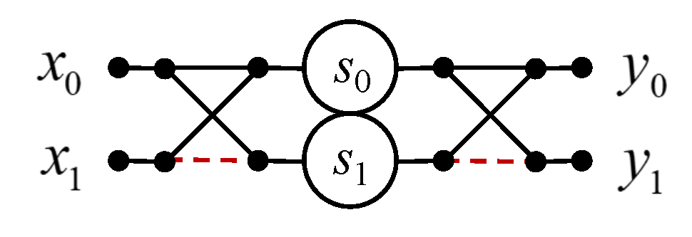
3.1. Circular Convolution for $N=2$

Let ${\mathit{X}}_{2\times 1}={[x_0,x_1]}^T$ and ${\mathit{H}}_{2\times 1}={[h_0,h_1]}^T$ be two-dimensional data vectors being convolved and ${\mathit{Y}}_{2\times 1}={[y_0,y_1]}^T$ be an output vector representing a circular convolution. The task is reduced to calculating the following product:

$${\mathit{Y}}_{2\times 1}={\mathit{H}}_2{\mathit{X}}_{2\times 1}$$

(4)

where:

$${\mathit{H}}_2=\left[\begin{array}{cc}{h}_0& h_1\\ h_1& h_0\end{array}\right],$$

Calculating (4) directly requires four multiplications and two additions. It is easy to see that the ${\mathit{H}}_2$ matrix has an unusual structure. Taking into account this specificity leads to the fact that the number of multiplications in the calculation of the two-point circular convolution can be reduced [7].

The optimized computational procedure for computing the two-point circular convolution is as follows:

$${\mathit{Y}}_{2\times 1}={\tilde{\mathit{H}}}_2{\mathit{D}}_2^{\left(2\right)}{\tilde{\mathit{H}}}_2{\mathit{X}}_{2\times 1}$$

(5)

where:

$${\tilde{\mathit{H}}}_2=\left[\begin{array}{cc}1& 1\\ 1& -1\end{array}\right],{\mathit{D}}_2^{\left(2\right)}=diag(s_0^{\left(2\right)},s_1^{\left(2\right)}),s_0^{\left(2\right)}=\frac{1}{2}(h_0+h_1),s_1^{\left(2\right)}=\frac{1}{2}(h_0-h_1)$$

Figure 1 shows a signal flow graph for the proposed algorithm, which also provides a simplified algorithmic structure of a fully parallel processing core for resource-effective implementation of the two-point circular convolution. All signal flow graphs are oriented from left to right. Straight lines denote the data circuits. The circles in these figures show the hardwired multipliers by a constant inscribed inside a circle. Points, where lines converge, denote adders, and dotted lines indicate the sign-change data circuits (datapaths with multiplication by −1).

Therefore, it only takes two multiplications and four additions to compute the two-point circular convolution. As for the arithmetic blocks, for a completely parallel hardware implementation of the processor core to compute the two-point convolution, you need two multipliers and four two-input adders, instead of four multipliers and two two-input adders in the case of a completely parallel implementation (4).

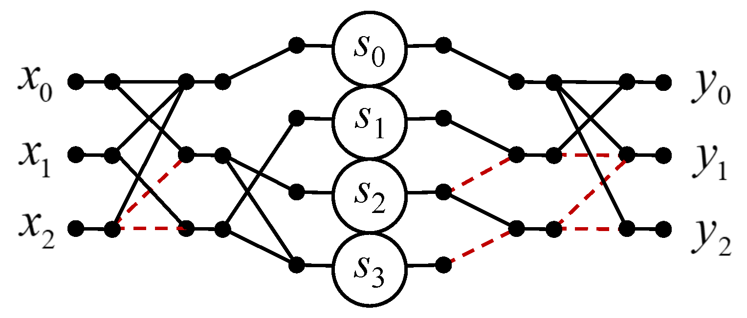
3.2. Circular Convolution for $N=3$

Let ${\mathit{X}}_{3\times 1}={[x_0,x_1,x_2]}^T$ and ${\mathit{H}}_{3\times 1}={[h_0,h_1,h_2]}^T$ be three-dimensional data vectors being convolved and ${\mathit{Y}}_{3\times 1}={[y_0,y_1,y_2]}^T$ be an output vector representing circular convolution for N = 3. The task is reduced to calculating the following product:

$${\mathit{Y}}_{3\times 1}={\mathit{H}}_3{\mathit{X}}_{3\times 1}$$

(6)

where:

$${\mathit{H}}_3=\left[\begin{array}{ccc}{h}_0& h_2& h_1\\ h_1& h_0& h_2\\ h_2& h_1& h_0\end{array}\right],$$

Calculating (6) directly requires nine multiplications and five additions. It is easy to see that the ${\mathit{H}}_3$ matrix has an unusual structure. Taking into account this specificity leads to the fact that the number of multiplications in the calculation of the three-point circular convolution can be reduced [7,8,11,27].

Therefore, the optimized computational procedure for computing the three-point circular convolution is as follows:

$${\mathit{Y}}_3^{\left(3\right)}={\tilde{\mathit{A}}}_3^{\left(3\right)}{\mathit{A}}_{3\times 4}^{\left(3\right)}{\mathit{D}}_4^{\left(3\right)}{\mathit{A}}_{4\times 3}^{\left(3\right)}{\mathit{A}}_3^{\left(3\right)}{\mathit{X}}_{3\times 1}$$

(7)

where:

$${\mathit{A}}_3^{\left(3\right)}=\left[\begin{array}{ccc}1& 1& 1\\ 1& -1& 0\\ 0& 1& -1\end{array}\right],{\mathit{A}}_{4\times 3}^{\left(3\right)}=\left[\begin{array}{ccc}1& 0& 0\\ 0& 1& 0\\ 0& 0& 1\\ 0& 1& 1\end{array}\right],$$

$${\mathit{A}}_{3\times 4}^{\left(3\right)}=\left[\begin{array}{cccc}1& 0& 0& 0\\ 0& 1& -1& 0\\ 0& 0& 1& 1\end{array}\right],{\tilde{\mathit{A}}}_3^{\left(3\right)}=\left[\begin{array}{ccc}1& 1& 0\\ 1& -1& -1\\ 1& 0& 1\end{array}\right],$$

$${\mathit{D}}_4^{\left(3\right)}=\mathrm{diag}\left({\mathrm{s}}_0^{\left(3\right)},{\mathrm{s}}_1^{\left(3\right)},{\mathrm{s}}_2^{\left(3\right)},{\mathrm{s}}_3^{\left(3\right)}\right),$$

$$s_0^{\left(3\right)}=\frac{1}{3}(h_0+h_1,+h_2),s_1^{\left(3\right)}=(h_0-h_1),s_2^{\left(3\right)}=(h_1-h_2),s_3^{\left(3\right)}=\frac{1}{3}(h_0+h_1-2h_2).$$

Figure 2 shows a signal flow graph of the proposed algorithm for the implementation of the three-point circular convolution.

As for the arithmetic blocks, for a completely parallel hardware implementation of the processor core to compute the three-point convolution (7), you need four multipliers and eleven two-input adders, instead of nine multipliers and six two-input adders in the case of a completely parallel implementation (6). Therefore, we have exchanged five multipliers for five two-input adders.

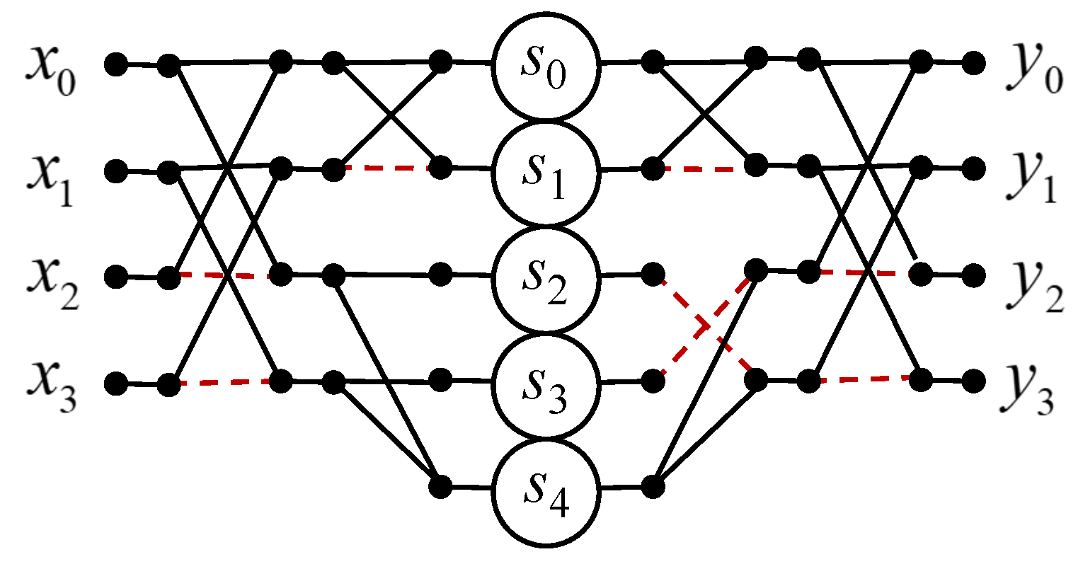
3.3. Circular Convolution for $N=4$

Let ${\mathit{X}}_{4\times 1}={[x_0,x_1,x_2,x_3]}^T$ and ${\mathit{H}}_{4\times 1}={[h_0,h_1,h_2,h_3]}^T$ be four-dimensional data vectors being convolved and ${\mathit{Y}}_{4\times 1}={[y_0,y_1,y_2,y_3]}^T$ be an output vector representing circular convolution for N = 4.

The task is reduced to calculating the following product:

$${\mathit{Y}}_{4\times 1}={\mathit{H}}_4{\mathit{X}}_{4\times 1}$$

(8)

where:

$${\mathit{H}}_4=\left[\begin{array}{cccc}{h}_0& h_3& h_2& h_1\\ h_1& h_0& h_3& h_2\\ h_2& h_1& h_0& h_3\\ h_3& h_2& h_1& h_0\end{array}\right].$$

Calculating (8) directly requires 16 multiplications and 12 additions. It is easy to see that the ${\mathit{H}}_4$ matrix has an unusual structure. Taking into account this specificity leads to the fact that the number of multiplications in the calculation of the four-point circular convolution can be reduced.

Therefore, the optimized computational procedure for computing the four-point circular convolution is as follows:

$${\mathit{Y}}_{4\times 1}={\mathit{A}}_4^{\left(4\right)}{\mathit{A}}_{4\times 5}^{\left(4\right)}{\mathit{D}}_5^{\left(4\right)}{\mathit{A}}_{5\times 4}^{\left(4\right)}{\mathit{A}}_4^{\left(4\right)}{\mathit{X}}_{4\times 1}$$

(9)

where:

$${\mathit{A}}_4^{\left(4\right)}={\tilde{\mathit{H}}}_2\otimes {\mathit{I}}_2=\left[\begin{array}{cccc}1& 0& 1& 0\\ 0& 1& 0& 1\\ 1& 0& -1& 0\\ 0& 1& 0& -1\end{array}\right],{\mathit{A}}_{5\times 4}^{\left(4\right)}={\tilde{\mathit{H}}}_2\oplus \left[\begin{array}{cc}1& 0\\ 0& 1\\ 1& 1\end{array}\right],$$

$${\mathit{A}}_{4\times 5}^{\left(4\right)}={\tilde{\mathit{H}}}_2\oplus \left[\begin{array}{ccc}0& -1& 1\\ -1& 0& 1\end{array}\right],$$

$${\mathit{D}}_5^{\left(4\right)}=diag(s_0^{\left(4\right)}{s}_1^{\left(4\right)},...,s_4^{\left(4\right)}),$$

$$s_0^{\left(4\right)}=(h_0+h_1+h_2+h_3)/4,s_1^{\left(4\right)}=(h_0-h_1+h_2-h_3)/4,$$

$$s_2^{\left(4\right)}=(h_0-h_1-h_2+h_3)/2,s_3^{\left(4\right)}=(h_0+h_1-h_2-h_3)/2,s_4^{\left(4\right)}=(h_0-h_2)/2,$$

where ${\mathit{I}}_N$ is an identity N matrix, ${\tilde{\mathit{H}}}_2$ is the 2 × 2 Hadamard matrix, and signs “⊗” and “⊕” denote the Kronecker product and direct sum of two matrices, respectively [30,31].

Figure 3 shows a signal flow graph of the proposed algorithm for the implementation of the four-point circular convolution.

As for the arithmetic blocks, to compute the four-point convolution (9), you need five multipliers and fifteen two-input adders, instead of sixteen multipliers and twelve two-input adders in the case of a completely parallel implementation (8). The proposed algorithm saves eleven multiplications at the cost of three extra additions compared to the ordinary matrix–vector multiplication method.

3.4. Circular Convolution for $N=5$

Let ${\mathit{X}}_{5\times 1}={[x_0,x_1,x_2,x_3,x_4]}^T$ and ${\mathit{H}}_{5\times 1}={[h_0,h_1,h_2,h_3,h_4]}^T$ be five-dimensional data vectors being convolved and ${\mathit{Y}}_{9\times 1}={[y_0,y_1,y_2,y_3,y_4]}^T$ be an output vector representing a circular convolution for N = 5.

The task is reduced to calculating the following product:

$${\mathit{Y}}_{5\times 1}={\mathit{H}}_5{\mathit{X}}_{5\times 1}$$

(10)

where:

$${\mathit{H}}_5=\left[\begin{array}{ccccc}{h}_0& h_4& h_3& h_2& h_1\\ h_1& h_0& h_4& h_3& h_2\\ h_2& h_1& h_0& h_4& h_3\\ h_3& h_2& h_1& h_0& h_4\\ h_4& h_3& h_2& h_1& h_0\end{array}\right],$$

Calculating (10) directly requires 25 multiplications and 20 additions. It is easy to see that the ${\mathit{H}}_5$ matrix has an unusual structure. Taking into account this specificity leads to the fact that the number of multiplications in the calculation of the five-point circular convolution can be reduced.

Therefore, an efficient algorithm for computing the five-point circular convolution can be represented using the following matrix–vector procedure:

$${\mathit{Y}}_{5\times 1}={\mathit{A}}_{5\times 7}^{\left(5\right)}{\mathit{A}}_{7\times 10}^{\left(5\right)}{\mathit{D}}_{10}^{\left(5\right)}{\mathit{A}}_{10\times 9}^{\left(5\right)}{\mathit{A}}_{9\times 5}^{\left(5\right)}{\mathit{A}}_5^{\left(5\right)}{\mathit{X}}_{5\times 1}$$

(11)

where:

$${\mathit{A}}_5^{\left(5\right)}=\left[\begin{array}{ccccc}1& 0& 0& 0& -1\\ 0& 1& 0& 0& -1\\ 0& 0& 1& 0& -1\\ 0& 0& 0& 1& -1\\ 1& 1& 1& 1& 1\end{array}\right],{\mathit{A}}_{9\times 5}^{\left(5\right)}=\left[\begin{array}{ccccc}1& 0& 0& 0& 0\\ 0& 1& 0& 0& 0\\ 1& 1& 0& 0& 0\\ 0& 0& 1& 0& 0\\ 0& 0& 0& 1& 0\\ 0& 0& 1& 1& 0\\ 1& 0& -1& 0& 0\\ 0& 1& 0& -1& 0\\ 0& 0& 0& 0& 1\end{array}\right],$$

$${\mathit{D}}_{16}^{\left(5\right)}=diag(s_0^{\left(5\right)}{s}_1^{\left(5\right)},\dots ,s_9^{\left(5\right)}),$$

$$s_0^{\left(5\right)}=(h_0-h_2+h_3-h_4)/4,s_1^{\left(5\right)}=(h_1-h_2+h_3-h_4)/4,$$

$$s_2^{\left(5\right)}=(3h_2-2h_1+2h_0-2h_3+3h_4)/5,s_3^{\left(5\right)}=(-h_0+h_1-h_2+h_3),$$

$$s_4^{\left(5\right)}=(-h_0+h_1-h_2+h_3),s_5^{\left(5\right)}=(3h_0-2h_1+3h_2-2h_3-2h_4)/5,$$

$$s_6^{\left(5\right)}=-h_2+h_3,s_7^{\left(5\right)}=h_1-h_2,s_8^{\left(5\right)}=(-h_0-h_1+4h_2-h_3-h_4)/5,$$

$$s_9^{\left(5\right)}=(h_0+h_1+h_2+h_3+h_4)/5,$$

$${\mathit{A}}_{10\times 9}^{\left(5\right)}=\left[\begin{array}{ccccccccc}1& 0& 0& 0& 0& 0& 0& 0& 0\\ 0& 1& 0& 0& 0& 0& 0& 0& 0\\ 0& 0& 1& 0& 0& 0& 0& 0& 0\\ 0& 0& 0& 1& 0& 0& 0& 0& 0\\ 0& 0& 0& 0& 1& 0& 0& 0& 0\\ 0& 0& 0& 0& 0& 1& 0& 0& 0\\ 0& 0& 0& 0& 0& 0& 1& 0& 0\\ 0& 0& 0& 0& 0& 0& 0& 1& 0\\ 0& 0& 1& 0& 0& -1& 0& 0& 0\\ 0& 0& 0& 0& 0& 0& 0& 0& 1\end{array}\right],$$

$${\mathit{A}}_{7\times 10}^{\left(5\right)}=\left[\begin{array}{cccccccccc}1& 0& 1& 0& 0& 0& 0& 0& 0& 0\\ 0& 1& 1& 0& 0& 0& 0& 0& 0& 0\\ 0& 0& 0& 1& 0& 1& 0& 0& 0& 0\\ 0& 0& 0& 0& 1& 1& 0& 0& 0& 0\\ 0& 0& 0& 0& 0& 0& 1& 0& 1& 0\\ 0& 0& 0& 0& 0& 0& 0& 1& 1& 0\\ 0& 0& 0& 0& 0& 0& 0& 0& 0& 1\end{array}\right],$$

$${\mathit{A}}_{5\times 7}^{\left(5\right)}=\left[\begin{array}{ccccccc}1& 0& 0& 0& -1& 0& 1\\ -1& -1& -1& -1& 0& 0& 0\\ 0& 0& 0& 1& 0& 1& 1\\ 0& 0& 1& 0& 1& 0& 1\\ 0& 1& 0& 0& 0& -1& 1\end{array}\right].$$

Figure 4 shows a data flow graph of the proposed algorithm for the implementation of the five-point circular convolution.

As for the arithmetic blocks, to compute the five-point convolution (11), you need ten multipliers, and thirty two-input adders, instead of twenty-five multipliers and twenty two-input adders in the case of a completely parallel implementation (10). The proposed algorithm saves 15 multiplications at the cost of 11 extra additions compared to the ordinary matrix–vector multiplication method.

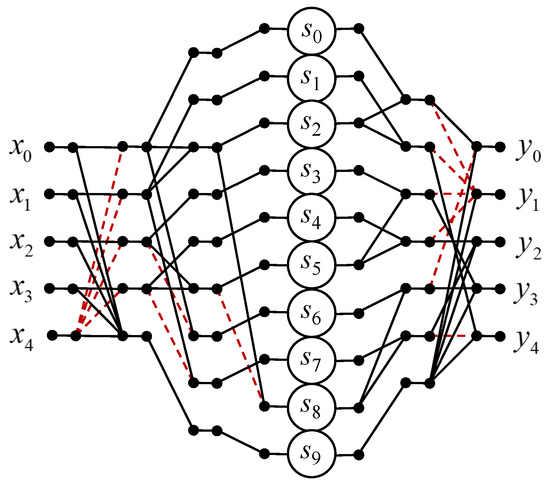
3.5. Circular Convolution for $N=6$

Let ${\mathit{X}}_{6\times 1}={[x_0,x_1,x_2,x_3,x_4,x_5]}^T$ and ${\mathit{H}}_{6\times 1}=[h_0,h_1,h_2,h_3,h_4,h_5]{,}^T$ be six-dimensional data vectors being convolved and ${\mathit{Y}}_{11\times 1}={[y_0,y_1,y_2,y_3,y_4,y_5]}^T$ be an output vector representing a circular convolution for N = 6.

The task is reduced to calculating the following product:

$${\mathit{Y}}_{6\times 1}={\mathit{H}}_6{\mathit{X}}_{6\times 1}$$

(12)

where:

$${\mathit{H}}_6=\left[\begin{array}{cccccc}{h}_0& h_5& h_4& h_3& h_2& h_1\\ h_1& h_0& h_5& h_4& h_3& h_2\\ h_2& h_1& h_0& h_5& h_4& h_3\\ h_3& h_2& h_1& h_0& h_5& h_4\\ h_4& h_3& h_2& h_1& h_0& h_5\\ h_5& h_4& h_3& h_2& h_1& h_0\end{array}\right],$$

Calculating (12) directly requires 36 multiplications and 30 additions. It is easy to see that the ${\mathit{H}}_6$ matrix has an unusual structure. Taking into account this specificity leads to the fact that the number of multiplications in the calculation of the six-point circular convolution can be reduced.

Therefore, an efficient algorithm for computing the six-point circular convolution can be represented using the following matrix–vector procedure:

$${\mathit{Y}}_{6\times 1}={\tilde{\mathit{P}}}_6^{\left(6\right)}{\mathit{A}}_6^{\left(6\right)}{\mathit{A}}_6^{\left(6\right)}{\mathit{A}}_{6\times 8}^{\left(6\right)}{\mathit{D}}_8^{\left(6\right)}{\mathit{A}}_{8\times 6}^{\left(6\right)}{\tilde{\mathit{A}}}_6^{\left(6\right)}{\mathit{A}}_6^{\left(6\right)}{\mathit{P}}_6^{\left(6\right)}{\mathit{X}}_{6\times 1}$$

(13)

where:

$${\mathit{P}}_6^{\left(6\right)}=\left[\begin{array}{cccccc}1& 0& 0& 0& 0& 0\\ 0& 0& 1& 0& 0& 0\\ 0& 0& 0& 0& 1& 0\\ 0& 0& 0& 1& 0& 0\\ 0& 0& 0& 0& 0& 1\\ 0& 1& 0& 0& 0& 0\end{array}\right],{\mathit{A}}_6^{\left(6\right)}={\tilde{\mathit{H}}}_2\otimes {\mathit{I}}_3=\left[\begin{array}{cccccc}1& 0& 0& 1& 0& 0\\ 0& 1& 0& 0& 1& 0\\ 0& 0& 1& 0& 0& 1\\ 1& 0& 0& -1& 0& 0\\ 0& 1& 0& 0& -1& 0\\ 0& 0& 1& 0& 0& -1\end{array}\right],$$

$${\mathit{D}}_8=diag(s_0^{\left(6\right)},s_1^{\left(6\right)},...,s_7^{\left(6\right)}),$$

$$s_0^{\left(6\right)}=h_0+h_3+h_4+h_1+h_2+h_5,s_1^{\left(6\right)}=3(h_4+h_1-h_0-h_3),$$

$$s_2^{\left(6\right)}=3(h_2+h_5-h_0-h_3),s_3^{\left(6\right)}=3(h_0+h_3)-(h_0+h_3+h_4+h_1+h_2+h_5),$$

$$s_4^{\left(6\right)}=h_0-h_3+h_4-h_1+h_2-h_5,s_5^{\left(6\right)}=3(h_4-h_1-h_0+h_3),$$

$$s_6^{\left(6\right)}=3(h_2-h_5-h_0+h_3),s_7^{\left(6\right)}=3(h_0+h_3)-(h_0-h_3+h_4-h_1+h_2-h_5),$$

$${\tilde{\mathit{A}}}_6^{\left(6\right)}=\left[\begin{array}{cccccc}1& 1& 1& 0& 0& 0\\ 1& -1& 0& 0& 0& 0\\ 1& 0& -1& 0& 0& 0\\ 0& 0& 0& 1& 1& 1\\ 0& 0& 0& 1& -1& 0\\ 0& 0& 0& 1& 0& -1\end{array}\right],\oplus {\mathit{I}}_5,{\tilde{\mathit{P}}}_6^{\left(6\right)}=\left[\begin{array}{cccccc}1& 0& 0& 0& 0& 0\\ 0& 0& 0& 0& 1& 0\\ 0& 0& 1& 0& 0& 0\\ 0& 0& 0& 1& 0& 0\\ 0& 1& 0& 0& 0& 0\\ 0& 0& 0& 0& 0& 1\end{array}\right].$$

Figure 5 shows a data flow graph of the proposed algorithm for the implementation of the six-point circular convolution.

As far as arithmetic blocks are concerned, eight multipliers and thirty-four two-input adders are needed for the completely parallel hardware implementation of the processor core to compute the six-point convolution (13), instead of thirty-six multipliers and thirty two-input adders in the case of a completely parallel implementation (12). The proposed algorithm saves twenty-eight multiplications at the cost of six extra additions compared to the ordinary matrix–vector multiplication method.

3.6. Circular Convolution for $N=7$

Let ${\mathit{X}}_{7\times 1}={[x_0,x_1,x_2,x_3,x_4,x_5,x_6]}^T$ and ${\mathit{H}}_{7\times 1}=[h_0,h_1,h_2,h_3,h_4,h_5,h_6]{,}^T$ be seven-dimensional data vectors being convolved and ${\mathit{Y}}_{7\times 1}={[y_0,y_1,y_2,y_3,y_4,y_5,y_6]}^T$ be an output vector representing a circular convolution for N = 7.

The task is reduced to calculating the following product:

$${\mathit{Y}}_{7\times 1}={\mathit{H}}_7{\mathit{X}}_{7\times 1}$$

(14)

$${\mathit{H}}_7=\left[\begin{array}{ccccccc}{h}_0& h_6& h_5& h_4& h_3& h_2& h_1\\ h_1& h_0& h_6& h_5& h_4& h_3& h_2\\ h_2& h_1& h_0& h_6& h_5& h_4& h_3\\ h_3& h_2& h_1& h_0& h_6& h_5& h_4\\ h_4& h_3& h_2& h_1& h_0& h_6& h_5\\ h{}_5& h{}_4& h_3& h_2& h_1& h_0& h_6\\ h_6& h_5& h_4& h_3& h_2& h_1& h_0\end{array}\right].$$

Calculating (14) directly requires 49 multiplications and 42 additions. It is easy to see that the ${\mathit{H}}_7$ matrix has an unusual structure. Taking into account this specificity leads to the fact that the number of multiplications in the calculation of the seven-point circular convolution can be reduced.

Therefore, an efficient algorithm for computing the seven-point circular convolution can be represented using the following matrix–vector procedure:

$${\mathit{Y}}_{7\times 1}={\mathit{A}}_{7\times 9}^{\left(7\right)}{\mathit{A}}_{9\times 10}^{\left(7\right)}{\mathit{A}}_{10\times 11}^{\left(7\right)}{\mathit{A}}_{11\times 12}^{\left(7\right)}{\mathit{A}}_{12\times 15}^{\left(7\right)}{\mathit{A}}_{15\times 11}^{\left(7\right)}{\mathit{A}}_{11}^{\left(7\right)}{\mathit{A}}_{11\times 16}^{\left(7\right)}{\mathit{D}}_{16}^{\left(7\right)}{\mathit{A}}_{16}^{\left(7\right)}{\mathit{A}}_{16\times 18}^{\left(7\right)}{\mathit{A}}_{18\times 11}^{\left(7\right)}{\mathit{A}}_{11\times 8}^{\left(7\right)}{\mathit{A}}_{8\times 7}^{\left(7\right)}{\mathit{X}}_{7\times 1}$$

(15)

where:

$${\mathit{A}}_{8\times 7}^{\left(7\right)}=\left[\begin{array}{ccccccc}1& 1& 1& 0& 0& 0& 0\\ 1& 0& 0& 0& 0& 0& -1\\ 0& 1& 0& 0& 0& 0& -1\\ 0& 0& 1& 0& 0& 0& -1\\ 0& 0& 0& 1& 0& 0& -1\\ 0& 0& 0& 0& 1& 0& -1\\ 0& 0& 0& 0& 0& 1& -1\\ 0& 0& 0& 0& 0& 0& 1\end{array}\right],{\mathit{A}}_{11\times 8}^{\left(7\right)}=\left[\begin{array}{cccccccc}1& 0& 0& 0& 0& 0& 0& 0\\ 1& 0& 0& 0& 0& 0& 0& 1\\ 0& 1& 0& 0& 0& 0& 0& 0\\ 0& -1& 0& 0& 1& 0& 0& 0\\ 0& 0& 0& 0& 1& 0& 0& 0\\ 0& 0& 1& 1& 0& 0& 0& 0\\ 0& 0& -1& 1& 0& 0& 0& 0\\ 0& 0& 0& 0& 0& 1& 1& 0\\ 0& 0& 0& 0& 0& -1& 1& 0\\ 0& 0& 0& 1& 0& 0& 0& 0\\ 0& 0& 0& 0& 0& 0& 1& 0\end{array}\right],$$

$${\mathit{A}}_{18\times 11}^{\left(7\right)}=\left[\begin{array}{ccccccccccc}1& 0& 0& 0& 0& 0& 0& 0& 0& 0& 0\\ 0& 1& 0& 0& 0& 0& 0& 0& 0& 0& 0\\ 0& 0& 1& 0& 0& 0& 0& 0& 0& 0& 0\\ 0& 0& 0& 1& 0& 0& 0& 0& 0& 0& 0\\ 0& 0& 0& 0& 1& 0& 0& 0& 0& 0& 0\\ 0& 0& 1& 0& 0& 1& 0& 0& 0& 0& 0\\ 0& 0& 1& 0& 0& 0& 1& 0& 0& 0& 0\\ 0& 0& 0& 0& 1& 0& 0& 1& 0& 0& 0\\ 0& 0& 0& 0& 1& 0& 0& 0& 1& 0& 0\\ 0& 0& 0& 0& 0& 1& 0& 0& 0& 0& 0\\ 0& 0& 0& 0& 0& 1& 0& 0& 0& 0& 0\\ 0& 0& 0& 0& 0& 0& 1& 0& 0& 0& 0\\ 0& 0& 0& 0& 0& 0& 0& 1& 0& 0& 0\\ 0& 0& 0& 0& 0& 0& 0& 1& 0& 0& 0\\ 0& 0& 0& 0& 0& 0& 0& 0& 1& 0& 0\\ 0& 0& 0& 0& 0& 0& 0& 0& 0& 1& 0\\ 0& 0& 0& 0& 0& 0& 0& 0& 0& -1& 1\\ 0& 0& 0& 0& 0& 0& 0& 0& 0& 0& 1\end{array}\right],$$

$${\mathit{A}}_{16\times 18}^{\left(7\right)}=\left[\begin{array}{cccccccccccccccccc}1& 0& 0& 0& 0& 0& 0& 0& 0& 0& 0& 0& 0& 0& 0& 0& 0& 0\\ 0& 1& 0& 0& 0& 0& 0& 0& 0& 0& 0& 0& 0& 0& 0& 0& 0& 0\\ 0& 0& 1& 0& 0& 0& 0& 0& 0& 0& 0& 0& 0& 0& 0& 0& 0& 0\\ 0& 0& 0& 1& 0& 0& 0& 0& 0& 0& 0& 0& 0& 0& 0& 0& 0& 0\\ 0& 0& 0& 0& 1& 0& 0& 0& 0& 0& 0& 0& 0& 0& 0& 0& 0& 0\\ 0& 0& 0& 0& 0& 1& 0& 0& 0& 0& 0& 0& 0& 0& 0& 0& 0& 0\\ 0& 0& 0& 0& 0& -1& 0& 1& 0& 0& 0& 0& 0& 0& 0& 0& 0& 0\\ 0& 0& 0& 0& 0& 0& 1& 0& 0& 0& 0& 0& 0& 0& 0& 0& 0& 0\\ 0& 0& 0& 0& 0& 0& 0& 1& 0& 0& 0& 0& 0& 0& 0& 0& 0& 0\\ 0& 0& 0& 0& 0& 0& -1& 0& 1& 0& 0& 0& 0& 0& 0& 0& 0& 0\\ 0& 0& 0& 0& 0& 0& 0& 0& 1& 0& 0& 0& 0& 0& 0& 0& 0& 0\\ 0& 0& 0& 0& 0& 1& 0& 0& 0& 1& 1& 1& 0& 0& 0& 0& 0& 0\\ 0& 0& 0& 0& 0& 0& 0& 1& 0& 0& 0& 0& 1& 1& 1& 0& 0& 0\\ 0& 0& 0& 0& 0& 0& 0& 0& 0& 0& 0& 0& 0& 0& 0& 1& 0& 0\\ 0& 0& 0& 0& 0& 0& 0& 0& 0& 0& 0& 0& 0& 0& 0& 0& 1& 0\\ 0& 0& 0& 0& 0& 0& 0& 0& 0& 0& 0& 0& 0& 0& 0& 0& 0& 1\end{array}\right],$$

$${\mathit{A}}_{16}^{\left(7\right)}=\left[\begin{array}{cccccccccccccccc}1& 1& 0& 0& 0& 0& 1& 0& 0& 0& 0& 0& 0& 0& 0& 0\\ 0& 0& 1& 0& 0& 0& 0& 0& 0& 0& 0& 0& 0& 0& 0& 0\\ 0& 0& 0& 1& 0& 0& 0& 0& 0& 0& 0& 0& 0& 0& 0& 0\\ 0& 0& 0& 0& 1& 0& 0& 0& 0& 0& 0& 0& 0& 0& 0& 0\\ 0& 0& 0& 0& 0& 1& 0& 0& 0& 0& 0& 0& 0& 0& 0& 0\\ 0& 0& 0& 0& 0& 0& 1& 0& 0& 0& 0& 0& 0& 0& 0& 0\\ 0& 0& 0& 0& 0& 0& 0& 1& 0& 0& 0& 0& 0& 0& 0& 0\\ 0& 0& 0& 0& 0& 0& 0& 0& 1& 0& 0& 0& 0& 0& 0& 0\\ 0& 0& 0& 0& 0& 0& 0& 0& 0& 1& 0& 0& 0& 0& 0& 0\\ 0& 0& 0& 0& 0& 0& 0& 0& 0& 0& 1& 0& 0& 0& 0& 0\\ 0& 0& 0& 0& 0& 0& 0& 0& 0& 0& 0& 1& 0& 0& 0& 0\\ 0& 0& 0& 0& 0& 0& 0& 0& 0& 0& 0& -1& 1& 0& 0& 0\\ 0& 0& 0& 0& 0& 0& 0& 0& 0& 0& 0& 0& 1& 0& 0& 0\\ 0& 0& 0& 0& 0& 0& 0& 0& 0& 0& 0& 0& 0& 1& 0& 0\\ 0& 0& 0& 0& 0& 0& 0& 0& 0& 0& 0& 0& 0& 0& 1& 0\\ 0& 0& 0& 0& 0& 0& 0& 0& 0& 0& 0& 0& 0& 0& 0& 1\end{array}\right],$$

$${\mathit{D}}_{16}^{\left(7\right)}=diag(s_0^{\left(7\right)},s_1^{\left(7\right)},...,s_{15}^{\left(7\right)}),$$

$$s_0^{\left(7\right)}=(h_6+h_5+h_4+h_3+2h_2+h_1+h_0)/7,$$

$$s_1^{\left(7\right)}=(-h_6-2h_5+3h_4-h_3-2h_2+h_1+2h_0)/2,s_2^{\left(7\right)}=(2h_4-h_3-2h_2+h_1)/2,$$

$$s_3^{\left(7\right)}=(-h_6+h_5+2h_4-h_3-2h_2+3h_1-h_0)/2,$$

$$s_4^{\left(7\right)}=(10h_6+3h_5-11h_4+10h_3+3h_2-11h_1-4h_0)/14,$$

$$s_5^{\left(7\right)}=(-2h_6-2h_5-2h_4+12h_3+5h_2-9h_1-2h_0)/14,$$

$$s_6^{\left(7\right)}=(2h_6+3h_5-h_4-2h_3+3h_2-h_1)/6,$$

$$s_7^{\left(7\right)}=(3h_6-11h_5-4h_4+10h_3+3h_2-11h_1+10h_0)/14,$$

$$s_8^{\left(7\right)}=(-2h_3+3h_2-h_1)/6,s_9^{\left(7\right)}=(3h_6-h_5-2h_3+3h_2-h_1-2h_0)/6,$$

$$s_{10}^{\left(7\right)}=(-h_6+h_4-h_3+h_1)/6,s_{11}^{\left(7\right)}=(-h_3+h_1)/6,s_{12}^{\left(7\right)}=(h_5-h_3+h_1-h_0)/6,$$

$$s_{13}^{\left(7\right)}=2h_6-h_5-2h_4+3h_3-2h_2-2h_1+h_0,s_{14}^{\left(7\right)}=2h_3-h_2-2h_1+h_0,$$

$$s_{15}^{\left(7\right)}=-h_6-2h_5+h_4+2h_3-h_2-2h_1+3h_0,$$

$${\mathit{A}}_{11\times 16}^{\left(7\right)}=\left[\begin{array}{cccccccccccccccc}1& 0& 0& 0& 0& 0& 0& 0& 0& 0& 0& 0& 0& 0& 0& 0\\ 0& 1& 1& 0& 0& 0& 0& 0& 0& 0& 0& 0& 0& 0& 0& 0\\ 0& 0& 0& 0& 1& 1& 0& 0& 0& 0& 0& 0& 0& 0& 0& 0\\ 0& 0& 0& 0& 0& 0& 1& 0& 1& 0& 0& 0& 0& 0& 0& 0\\ 0& 0& 0& 0& 0& 0& 0& 0& 0& 0& 1& 1& 0& 0& 0& 0\\ 0& 0& 0& 0& 0& 0& 0& 0& 0& 0& 0& 0& 0& 1& 1& 0\\ 0& 0& -1& 1& 0& 0& 0& 0& 0& 0& 0& 0& 0& 0& 0& 0\\ 0& 0& 0& 0& 0& -1& 0& 1& 0& 0& 0& 0& 0& 0& 0& 0\\ 0& 0& 0& 0& 0& 0& 0& 0& -1& 1& 0& 0& 0& 0& 0& 0\\ 0& 0& 0& 0& 0& 0& 0& 0& 0& 0& 0& -1& 1& 0& 0& 0\\ 0& 0& 0& 0& 0& 0& 0& 0& 0& 0& 0& 0& 0& 0& -1& 1\end{array}\right],$$

$${\mathit{A}}_{11}^{\left(7\right)}=\left[\begin{array}{ccccccccccc}1& 0& 0& 0& 0& 0& 0& 0& 0& 0& 0\\ 0& 1& 0& 0& 0& 0& 0& 0& 0& 0& 0\\ 0& 0& 1& 0& 1& 0& 0& 0& 0& 0& 0\\ 0& 0& 0& 1& 0& 0& 0& 0& 0& 0& 0\\ 0& 0& 0& 0& 1& 0& 0& 0& 0& 0& 0\\ 0& 0& 0& 0& 0& 1& 0& 0& 0& 0& 0\\ 0& 0& 0& 0& 0& 0& 1& 0& 0& 0& 0\\ 0& 0& 0& 0& 0& 0& 0& 1& 0& 1& 0\\ 0& 0& 0& 0& 0& 0& 0& 0& 1& 0& 0\\ 0& 0& 0& 0& 0& 0& 0& 0& 0& 1& 0\\ 0& 0& 0& 0& 0& 0& 0& 0& 0& 0& 1\end{array}\right],$$

$${\mathit{A}}_{15\times 11}^{\left(7\right)}=\left[\begin{array}{ccccccccccc}1& 0& 0& 0& 0& 0& 0& 0& 0& 0& 0\\ 0& 1& 0& 0& 0& 0& 0& 0& 0& 0& 0\\ 0& 0& 1& 1& 0& 0& 0& 0& 0& 0& 0\\ 0& 0& 1& 0& 1& 0& 0& 0& 0& 0& 0\\ 0& 0& 0& 1& 0& 0& 0& 0& 0& 0& 0\\ 0& 0& 0& 0& 1& 0& 0& 0& 0& 0& 0\\ 0& 0& 0& 0& 1& 0& 0& 0& 0& 0& 0\\ 0& 0& 0& 0& 0& 1& 0& 0& 0& 0& 0\\ 0& 0& 0& 0& 0& 0& 1& 0& 0& 0& 0\\ 0& 0& 0& 0& 0& 0& 0& 1& 0& 0& 0\\ 0& 0& 0& 0& 0& 0& 0& 1& 0& 1& 0\\ 0& 0& 0& 0& 0& 0& 0& 0& 1& 0& 0\\ 0& 0& 0& 0& 0& 0& 0& 0& 0& 1& 0\\ 0& 0& 0& 0& 0& 0& 0& 0& 0& 1& 0\\ 0& 0& 0& 0& 0& 0& 0& 0& 0& 0& 1\end{array}\right],$$

$${\mathit{A}}_{12\times 15}^{\left(7\right)}=\left[\begin{array}{ccccccccccccccc}1& 0& 0& 0& 0& 0& 0& 0& 0& 0& 0& 0& 0& 0& 0\\ 0& 1& 1& 0& 0& 0& 0& 0& 0& 0& 0& 0& 0& 0& 0\\ 0& 0& 0& 1& 0& 0& 0& 0& 0& 0& 0& 0& 0& 0& 0\\ 0& 0& 0& 1& -1& 0& 0& 0& 0& 0& 0& 0& 0& 0& 0\\ 0& 0& 0& 1& 0& 1& 1& 1& 0& 0& 0& 0& 0& 0& 0\\ 0& 0& 0& 0& 1& 0& 0& 0& 0& 0& 0& 0& 0& 0& 0\\ 0& 0& 0& 0& 0& 0& 0& 0& 1& 0& 0& 0& 0& 0& 0\\ 0& 0& 0& 0& 0& 0& 0& 0& 0& 1& 0& 0& 0& 0& 0\\ 0& 0& 0& 0& 0& 0& 0& 0& 0& 0& 1& 0& 0& 0& 0\\ 0& 0& 0& 0& 0& 0& 0& 0& 0& 0& 1& -1& 0& 0& 0\\ 0& 0& 0& 0& 0& 0& 0& 0& 0& 0& 1& 0& 1& 1& 1\\ 0& 0& 0& 0& 0& 0& 0& 0& 0& 0& 0& 1& 0& 0& 0\end{array}\right],$$

$${\mathit{A}}_{11\times 12}^{\left(7\right)}=\left[\begin{array}{cccccccccccc}1& 0& 0& 0& 0& 0& 0& 0& 0& 0& 0& 0\\ 0& 1& 0& 0& 0& 0& 0& 0& 0& 0& 0& 0\\ 0& -1& -1& 0& -1& 0& 0& 0& 0& 0& 0& 0\\ 0& 0& 0& 1& 0& 0& 0& 0& 0& 0& 0& 0\\ 0& 0& 0& 0& 1& 1& 0& 0& 0& 0& 0& 0\\ 0& 0& 0& 0& 0& 0& 1& 0& 0& 0& 0& 0\\ 0& 0& 0& 0& 0& 0& 0& 0& 1& 0& 0& 0\\ 0& 0& 0& 0& 0& 0& 0& 0& 0& 1& 0& 0\\ 0& 0& 0& 0& 0& 0& 0& 0& 0& 0& 1& 1\\ 0& 0& 0& 0& 0& 0& 0& 1& 0& 0& 0& 1\\ 0& 0& 0& 0& 0& 0& 0& 0& 0& 0& 1& 0\end{array}\right],$$

$${\mathit{A}}_{10\times 11}^{\left(7\right)}=\left[\begin{array}{ccccccccccc}1& 0& 0& 0& 0& 0& 0& 0& 0& 0& 0\\ 0& 1& 0& 0& 0& 0& 0& 0& 0& 0& 0\\ 0& 0& 1& 0& 0& 0& 0& 0& 0& 0& 0\\ 0& 0& 0& 1& 0& 0& 0& 0& 0& 0& 0\\ 0& 0& 0& 0& 1& 0& 0& 0& 0& 0& 0\\ 0& 0& 0& 0& 0& 1& 0& 0& 0& 1& 0\\ 0& 0& 0& 0& 0& 0& 1& 0& 0& 0& 0\\ 0& 0& 0& 0& 0& 0& 0& 1& 0& 0& 0\\ 0& 0& 0& 0& 0& 0& 0& 0& 1& 0& 0\\ 0& 0& 0& 0& 0& 0& 0& 0& 0& 0& 1\end{array}\right],$$

$${\mathit{A}}_{9\times 10}^{\left(7\right)}=\left[\begin{array}{cccccccccc}1& 0& 0& 0& 0& 0& 0& 0& 0& 0\\ 0& 1& 0& 0& 0& 0& 0& 0& 0& 0\\ 0& 0& 1& 0& 0& 0& 0& 0& 0& 0\\ 0& 0& 0& 1& 0& 0& 0& 0& 0& 0\\ 0& 0& 0& 0& 1& 0& 0& 0& 0& 0\\ 0& 0& 0& 0& 0& 1& 0& 0& 0& 0\\ 0& 0& 0& 0& 0& -1& -1& 0& 0& -1\\ 0& 0& 0& 0& 0& 0& 0& 1& 0& 0\\ 0& 0& 0& 0& 0& 0& 0& 0& 1& 0\end{array}\right],$$

$${\mathit{A}}_{7\times 9}^{\left(7\right)}=\left[\begin{array}{ccccccccc}1& 0& 0& 0& 0& 0& 0& 1& 0\\ 1& 0& 0& 0& 0& 1& 0& 0& 0\\ 1& 0& 0& 0& 1& 0& 0& 0& 0\\ 1& 0& 0& 1& 0& 0& 0& 0& 0\\ 1& 1& 0& 0& 0& 0& 0& 0& 0\\ 1& 0& 1& 0& 0& 0& 1& 0& 0\\ 1& 0& 0& 0& 0& 0& 0& 0& 1\end{array}\right].$$

Figure 6 shows a data flow graph of the proposed algorithm for the implementation of the seven-point circular convolution.

As far as arithmetic blocks are concerned, sixteen multipliers and sixty-eight two-input adders are needed for the completely parallel hardware implementation of the processor core to compute the seven-point convolution (15), instead of forty-nine multipliers and forty-two two-input adders in the case of a completely parallel implementation (14). The proposed algorithm saves 33 multiplications at the cost of 26 extra additions compared to the ordinary matrix–vector multiplication method.

3.7. Circular Convolution for $N=8$

Let ${\mathit{X}}_{8\times 1}={[x_0,x_1,x_2,x_3,x_4,x_5,x_6,x_7]}^T$ and ${\mathit{H}}_{8\times 1}=[h_0,h_1,h_2,h_3,h_4,h_5,h_6,h_7]{,}^T$ be eight-dimensional data vectors being convolved and ${\mathit{Y}}_{8\times 1}={[y_0,y_1,y_2,y_3,y_4,y_5,y_6,y_7]}^T$ be an output vector representing a circular convolution for N = 8.

The task is reduced to calculating the following product:

$${\mathit{Y}}_{8\times 1}={\mathit{H}}_8{\mathit{X}}_{8\times 1}$$

(16)

$${\mathit{H}}_8=\left[\begin{array}{cccccccc}{h}_0& h_7& h_6& h_5& h_4& h_3& h_2& h_1\\ h_1& h_0& h_7& h_6& h_5& h_4& h_3& h_2\\ h_2& h_1& h_0& h_7& h_6& h_5& h_4& h_3\\ h_3& h_2& h_1& h_0& h_7& h_6& h_5& h_4\\ h_4& h_3& h_2& h_1& h_0& h{}_7& h_6& h_5\\ h_5& h_4& h_3& h_2& h_1& h_0& h_7& h_6\\ h_6& h_5& h_4& h_3& h{}_2& h_1& h_0& h_7\\ h_7& h_6& h_5& h_4& h_3& h_2& h_1& h_0\end{array}\right].$$

Calculating (16) directly requires 64 multiplications and 56 additions. It is easy to see that the ${\mathit{H}}_8$ matrix has an unusual structure. Taking into account this specificity leads to the fact that the number of multiplications in the calculation of the eight-point circular convolution can be reduced.

Therefore, an efficient algorithm for computing the eight-point circular convolution can be represented using the following matrix–vector procedure:

$${\mathit{Y}}_{8\times 1}={\mathit{P}}_8^{\left(8\right)}{\mathit{A}}_8^{\left(8\right)}{\mathit{A}}_{8\times 10}^{\left(8\right)}{\mathit{A}}_{10\times 14}^{\left(8\right)}{\mathit{D}}_{14}^{\left(8\right)}{\mathit{A}}_{14\times 10}^{\left(8\right)}{\mathit{A}}_{10\times 8}^{\left(8\right)}{\mathit{A}}_8^{\left(8\right)}{\mathit{X}}_{8\times 1}$$

(17)

where:

$${\mathit{A}}_8^{\left(8\right)}={\tilde{\mathit{H}}}_2\otimes {\mathit{I}}_4=\left[\begin{array}{cccccccc}1& 0& 0& 0& 1& 0& 0& 0\\ 0& 1& 0& 0& 0& 1& 0& 0\\ 0& 0& 1& 0& 0& 0& 1& 0\\ 0& 0& 0& 1& 0& 0& 0& 1\\ 1& 0& 0& 0& -1& 0& 0& 0\\ 0& 1& 0& 0& 0& -1& 0& 0\\ 0& 0& 1& 0& 0& 0& -1& 0\\ 0& 0& 0& 1& 0& 0& 0& -1\end{array}\right],$$

$${\mathit{A}}_{10\times 8}^{\left(8\right)}=({\tilde{\mathit{H}}}_2\otimes {\mathit{I}}_2)\oplus \left[\begin{array}{cc}{\mathit{I}}_2& {\mathbf{0}}_2\\ {\mathbf{0}}_2& {\mathit{I}}_2\\ {\mathit{I}}_2& {\mathit{I}}_2\end{array}\right],{\mathit{A}}_{14\times 10}^{\left(8\right)}={\tilde{\mathit{H}}}_2\oplus \left({\mathit{I}}_4\otimes \left[\begin{array}{cc}1& 0\\ 0& 1\\ 1& 1\end{array}\right]\right),$$

$${\mathit{D}}_{14}^{\left(8\right)}=diag(s_0^{\left(8\right)},s_1^{\left(8\right)},...,s_{13}^{\left(8\right)}),$$

$$s_0^{\left(8\right)}=\frac{1}{8}(h_0+h_1+h_2+h_3+h_4+h_5+h_6+h_7),$$

$$s_1^{\left(8\right)}=\frac{1}{8}(h_0-h_1+h_2-h_3+h_4-h_5+h_6-h_7),$$

$$s_2^{\left(8\right)}=\frac{1}{4}(-h_0+h_1+h_2-h_3-h_4+h_5+h_6-h_7),$$

$$s_3^{\left(8\right)}=\frac{1}{4}(-h_0-h_1+h_2+h_3-h_4-h_5+h_6+h_7),s_4^{\left(8\right)}=\frac{1}{4}(h_0-h_2+h_4-h_6),$$

$$s_5^{\left(8\right)}=\frac{1}{2}(h_0-h_1-h_2+h_3-h_4+h_5+h_6-h_7),$$

$$s_6^{\left(8\right)}=\frac{1}{2}(h_0+h_1-h_2+h_3-h_4-h_5+h_6-h_7),s_7^{\left(8\right)}=\frac{1}{2}(-h_0+h_2+h_4-h_6),$$

$$s_8^{\left(8\right)}=\frac{1}{2}(h_0-h_1+h_2-h_3-h_4+h_5-h_6+h_7),$$

$$s_9^{\left(8\right)}=\frac{1}{2}(h_0-h_1+h_2+h_3-h_4+h_5-h_6-h_7),s_{10}^{\left(8\right)}=\frac{1}{2}(-h_0-h_2+h_4+h_6),$$

$$s_{11}^{\left(8\right)}=\frac{1}{2}(-h_0+h_1+h_4-h_5),s_{12}^{\left(8\right)}=\frac{1}{2}(-h_0-h_3+h_4+h_7),s_{13}^{\left(8\right)}=\frac{1}{2}(h_0-h_4),$$

$${\mathit{A}}_{10\times 14}^{\left(8\right)}={\tilde{\mathit{H}}}_2\oplus \left({\mathit{I}}_4\otimes \left[\begin{array}{ccc}0& 1& 1\\ 1& 0& 1\end{array}\right]\right),{\mathit{A}}_{8\times 10}^{\left(8\right)}=({\tilde{\mathit{H}}}_2\otimes {\mathit{I}}_2)\oplus \left[\begin{array}{ccc}{\mathbf{0}}_2& {\mathit{I}}_2& {\mathit{I}}_2\\ {\mathit{I}}_2& {\mathbf{0}}_2& {\mathit{I}}_2\end{array}\right],$$

$${\mathit{P}}_8^{\left(8\right)}=\left[\begin{array}{cc}{\mathbf{0}}_{5\times 3}& {\mathit{I}}_5\\ {\mathit{I}}_3& {\mathbf{0}}_{3\times 5}\end{array}\right]=\left[\begin{array}{cccccccc}0& 0& 0& 1& 0& 0& 0& 0\\ 0& 0& 0& 0& 1& 0& 0& 0\\ 0& 0& 0& 0& 0& 1& 0& 0\\ 0& 0& 0& 0& 0& 0& 1& 0\\ 0& 0& 0& 0& 0& 0& 0& 1\\ 1& 0& 0& 0& 0& 0& 0& 0\\ 0& 1& 0& 0& 0& 0& 0& 0\\ 0& 0& 1& 0& 0& 0& 0& 0\end{array}\right].$$

Figure 7 shows a data flow graph of the proposed algorithm for the implementation of the eight-point circular convolution.

As far as arithmetic blocks are concerned, fourteen multipliers and forty-six two-input adders are needed for the completely parallel hardware implementation of the processor core to compute the eight-point convolution (17), instead of sixty-four multipliers and fifty-six two-input adders in the case of a completely parallel implementation (16). The proposed algorithm saves 50 multiplications and 10 additions compared to the ordinary matrix–vector multiplication method.

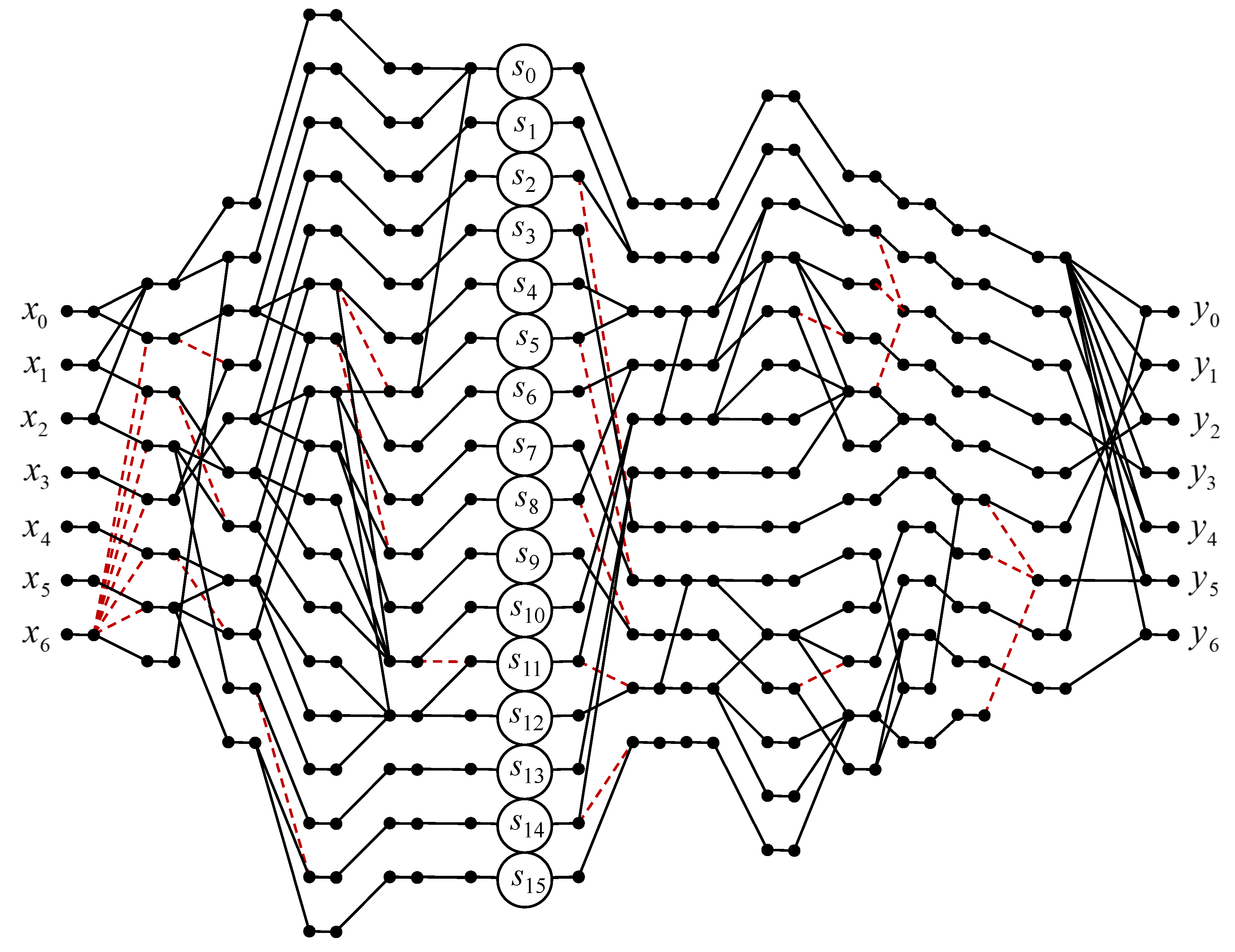
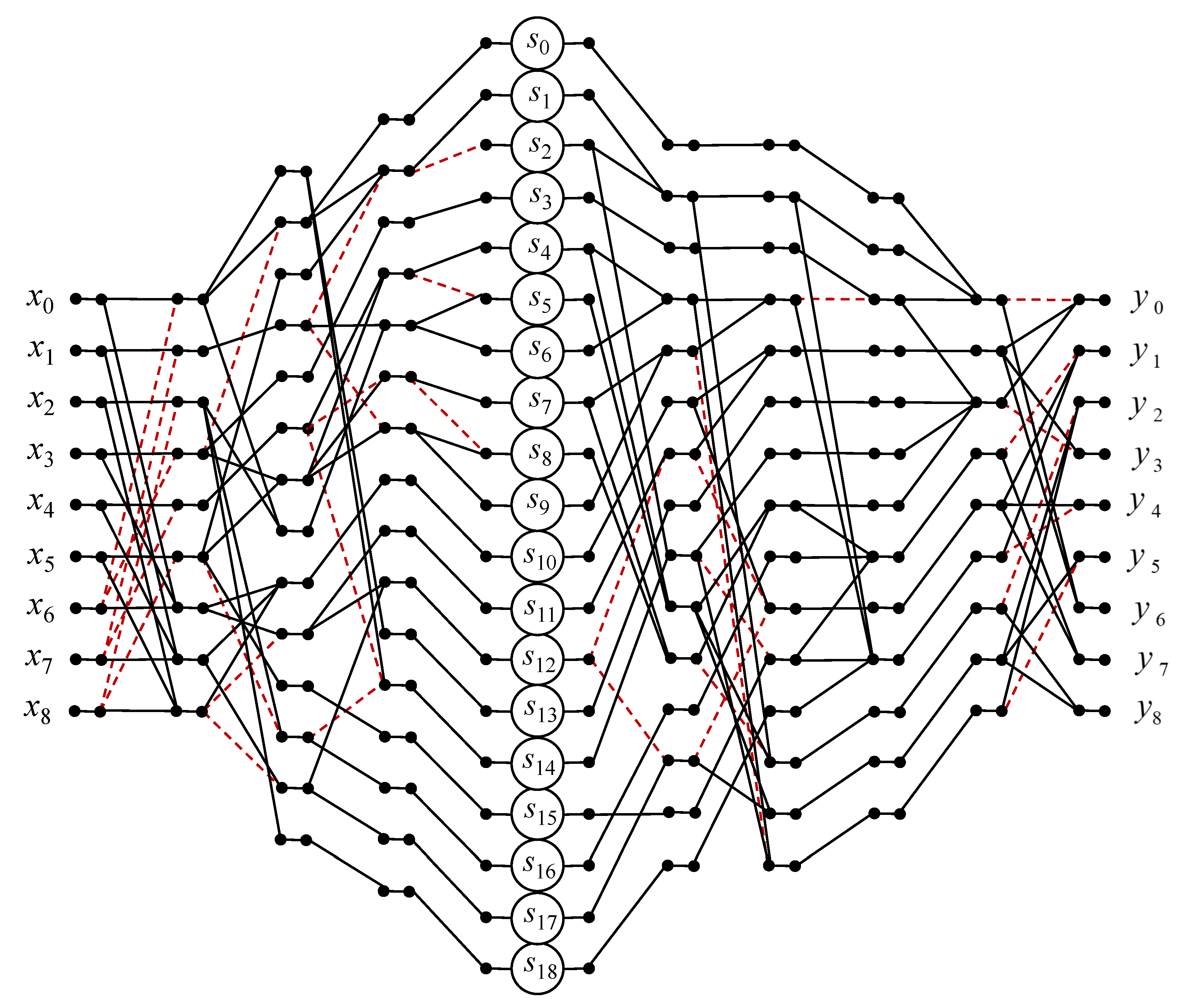
3.8. Circular Convolution for $N=9$

Let ${\mathit{X}}_{9\times 1}={[x_0,x_1,x_2,x_3,x_4,x_5,x_6,x_7,x_8]}^T$ and ${\mathit{H}}_{9\times 1}={[h_0,h_1,h_2,h_3,h_4,h_5,h_6,h_7,h_8]}^T$ be nine-dimensional data vectors being convolved and ${\mathit{Y}}_{9\times 1}={[y_0,y_1,y_2,y_3,y_4,y_5,y_6,y_7,y_8]}^T$ be an output vector representing a circular convolution for N = 9.

The task is reduced to calculating the following product:

$${\mathit{Y}}_{9\times 1}={\mathit{H}}_9{\mathit{X}}_{9\times 1}$$

(18)

$${\mathit{H}}_9=\left[\begin{array}{ccccccccc}{h}_0& h_8& h_7& h_6& h_5& h_4& h_3& h_2& h_1\\ h_1& h_0& h_8& h_7& h_6& h_5& h_4& h_3& h_2\\ h_2& h_1& h_0& h_8& h_7& h_6& h_5& h_4& h_3\\ h_3& h_2& h_1& h_0& h_8& h_7& h_6& h_5& h_4\\ h_4& h_3& h_2& h_1& h_0& h_8& h_7& h_6& h_5\\ h_5& h_4& h_3& h_2& h_1& h_0& h_8& h_7& h_6\\ h_6& h_5& h_4& h_3& h_2& h_1& h_0& h_8& h_7\\ h_7& h_6& h_5& h_4& h_3& h_2& h_1& h_0& h_8\\ y_8& h_7& h_6& h_5& h_4& h_3& h_2& h_1& h_0\end{array}\right].$$

Calculating (18) directly requires 81 multiplications and 72 additions. It is easy to see that the ${\mathit{H}}_9$ matrix has an unusual structure. Taking into account this specificity leads to the fact that the number of multiplications in the calculation of the nine-point circular convolution can be reduced.

Therefore, an efficient algorithm for computing the nine-point circular convolution can be represented using the following matrix–vector procedure:

$${\mathit{Y}}_{9\times 1}={\tilde{\mathit{A}}}_9^{\left(9\right)}{\mathit{A}}_{9\times 13}^{\left(9\right)}{\mathit{A}}_{13\times 15}^{\left(9\right)}{\mathit{A}}_{15}^{\left(9\right)}{\mathit{A}}_{15\times 19}^{\left(9\right)}{\mathit{D}}_{19}^{\left(9\right)}{\mathit{A}}_{19\times 16}^{\left(9\right)}{\mathit{A}}_{16\times 14}^{\left(9\right)}{\mathit{A}}_{14\times 9}^{\left(9\right)}{\mathit{A}}_9^{\left(9\right)}{\mathit{X}}_{9\times 1}$$

(19)

where:

$${\mathit{A}}_9^{\left(9\right)}=\left[\begin{array}{ccccccccc}1& 0& 0& 0& 0& 0& -1& 0& 0\\ 0& 1& 0& 0& 0& 0& 0& -1& 0\\ 0& 0& 1& 0& 0& 0& 0& 0& -1\\ 0& 0& 0& 1& 0& 0& -1& 0& 0\\ 0& 0& 0& 0& 1& 0& 0& -1& 0\\ 0& 0& 0& 0& 0& 1& 0& 0& -1\\ 1& 0& 0& 1& 0& 0& 1& 0& 0\\ 0& 1& 0& 0& 1& 0& 0& 1& 0\\ 0& 0& 1& 0& 0& 1& 0& 0& 1\end{array}\right],$$

$${\mathit{A}}_{14\times 9}^{\left(9\right)}=\left[\begin{array}{ccccccccc}1& 0& 0& 0& 0& 0& 0& 0& 0\\ 1& 0& 0& -1& 0& 0& 0& 0& 0\\ 0& 0& 0& 0& 0& 1& 0& 0& 0\\ 0& 1& 0& 0& 0& 0& 0& 0& 0\\ 0& 0& 0& 1& 0& 0& 0& 0& 0\\ 0& 0& 0& 0& 1& 0& 0& 0& 0\\ 0& 0& 0& 1& 0& 1& 0& 0& 0\\ 1& 0& 1& 0& 0& 0& 0& 0& 0\\ 0& 0& 0& 0& 0& 0& 1& 1& 1\\ 0& 0& 0& 0& 0& 0& 1& 0& -1\\ 0& 0& 0& 0& 0& 1& 0& 0& 0\\ 0& 0& 1& 0& 0& -1& 0& 0& 0\\ 0& 0& 0& 0& 0& 0& 0& 1& -1\\ 0& 0& 1& 0& 0& 0& 0& 0& 0\end{array}\right],$$

$${\mathit{A}}_{16\times 14}^{\left(9\right)}=\left[\begin{array}{cccccccccccccc}0& 1& 0& 0& 0& 0& 0& 0& 0& 0& 0& 0& 0& 0\\ 0& 1& 1& -1& 0& 0& 0& 0& 0& 0& 0& 0& 0& 0\\ 0& 0& 0& 0& 1& 0& 0& 0& 0& 0& 0& 0& 0& 0\\ 0& 0& 0& 0& 0& 1& 1& 0& 0& 0& 0& 0& 0& 0\\ 0& 0& 0& 1& 0& 0& 0& 1& 0& 0& 0& 0& 0& 0\\ 0& 0& 0& 0& 0& -1& 1& 0& 0& 0& 0& 0& 0& 0\\ 0& 0& 0& -1& 0& 0& 1& 0& 0& 0& 0& 0& 0& 0\\ 0& 0& 0& 0& 0& 0& 0& 0& 1& 0& 0& 0& 0& 0\\ 0& 0& 0& 0& 0& 0& 0& 0& 0& 1& 0& 0& 0& 0\\ 0& 0& 0& 0& 0& 0& 0& 0& 0& 1& 0& 0& 1& 0\\ 1& 0& 0& 0& 0& 0& 0& 0& 0& 0& 0& 0& 0& 0\\ 1& 0& 0& 0& 0& -1& 0& 0& 0& 0& 0& -1& 0& 0\\ 0& 0& 0& 0& 0& 0& 0& 0& 0& 0& 1& 0& 0& 0\\ 0& 0& 0& 0& 0& 0& 0& 0& 0& 0& 0& 1& 0& 0\\ 0& 0& 0& 0& 0& 0& 0& 0& 0& 0& 0& 0& 1& 0\\ 0& 0& 0& 0& 0& 0& 0& 0& 0& 0& 0& 0& 0& 1\end{array}\right],$$

$${\mathit{A}}_{19\times 16}^{\left(9\right)}=\left[\begin{array}{cccccccccccccccc}1& 0& 0& 0& 0& 0& 0& 0& 0& 0& 0& 0& 0& 0& 0& 0\\ 0& 1& 0& 0& 0& 0& 0& 0& 0& 0& 0& 0& 0& 0& 0& 0\\ 0& -1& 0& 0& 0& 0& 0& 0& 0& 0& 0& 1& 0& 0& 0& 0\\ 0& 0& 1& 0& 0& 0& 0& 0& 0& 0& 0& 0& 0& 0& 0& 0\\ 0& 0& 0& 1& 0& 0& 0& 0& 0& 0& 0& 0& 0& 0& 0& 0\\ 0& 0& 0& -1& 1& 0& 0& 0& 0& 0& 0& 0& 0& 0& 0& 0\\ 0& 0& 0& 0& 1& 0& 0& 0& 0& 0& 0& 0& 0& 0& 0& 0\\ 0& 0& 0& 0& 0& 1& 0& 0& 0& 0& 0& 0& 0& 0& 0& 0\\ 0& 0& 0& 0& 0& -1& 1& 0& 0& 0& 0& 0& 0& 0& 0& 0\\ 0& 0& 0& 0& 0& 0& 1& 0& 0& 0& 0& 0& 0& 0& 0& 0\\ 0& 0& 0& 0& 0& 0& 0& 1& 0& 0& 0& 0& 0& 0& 0& 0\\ 0& 0& 0& 0& 0& 0& 0& 0& 1& 0& 0& 0& 0& 0& 0& 0\\ 0& 0& 0& 0& 0& 0& 0& 0& 0& 1& 0& 0& 0& 0& 0& 0\\ 0& 0& 0& 0& 0& 0& 0& 0& 0& 0& 1& 0& 0& 0& 0& 0\\ 0& 0& 0& 0& 0& 0& 0& 0& 0& 0& 0& 1& 0& 0& 0& 0\\ 0& 0& 0& 0& 0& 0& 0& 0& 0& 0& 0& 0& 1& 0& 0& 0\\ 0& 0& 0& 0& 0& 0& 0& 0& 0& 0& 0& 0& 0& 1& 0& 0\\ 0& 0& 0& 0& 0& 0& 0& 0& 0& 0& 0& 0& 0& 0& 1& 0\\ 0& 0& 0& 0& 0& 0& 0& 0& 0& 0& 0& 0& 0& 0& 0& 1\end{array}\right]$$

$${\mathit{D}}_{19}^{\left(9\right)}=diag(s_0^{\left(9\right)},s_1^{\left(9\right)},...,s_{18}^{\left(9\right)}),$$

$$s_0^{\left(9\right)}=b_{17}=\frac{1}{3}(2b_0-b_2+b_4),s_1^{\left(9\right)}=b_{23}=\frac{1}{9}(-b_0+b_2-b_3+b_5),$$

$$s_2^{\left(9\right)}=b_{24}=b_{23}-b_{22},s_3^{\left(9\right)}=b_{16}=\frac{1}{3}(2b_0+b_1-b_2-2b_3+b_5),$$

$$s_4^{\left(9\right)}=b_{10}=\frac{1}{18}(b_0+3b_1+2b_2-2b_3-3b_4-b_5),s_5^{\left(9\right)}=b_{12}=b_{10}+b_{11},$$

$$s_6^{\left(9\right)}=b_{11}=\frac{1}{18}(b_0-b_2+b_3+3b_4+2b_5),s_7^{\left(9\right)}=b_{13}=\frac{1}{6}(-b_0+b_1-b_4+b_5),$$

$$s_8^{\left(9\right)}=b_{15}=b_{13}+b_{14},s_9^{\left(9\right)}=b_{14}=\frac{1}{6}(b_0-b_2-b_3+b_4),s_{10}^{\left(9\right)}=b_9=\frac{1}{9}(b_6+b_7+b_8),$$

$$s_{11}^{\left(9\right)}=b_{25}=\frac{1}{3}(b_6-b_8),s_{12}^{\left(9\right)}=b_{27}=\frac{1}{3}(b_{25}+b_{26}),s_{13}^{\left(9\right)}=b_{18}=b_{17}-b_{16},$$

$$s_{14}^{\left(9\right)}=b_{22}=\frac{1}{9}(b_0-b_2-2b_3+2b_5),s_{15}^{\left(9\right)}=b_{19}=\frac{1}{3}(b_0-b_1-2b_2+b_4),$$

$$s_{16}^{\left(9\right)}=b_{20}=\frac{1}{3}(-b_1+b_3-2b_5),s_{17}^{\left(9\right)}=b_{26}=\frac{1}{3}(b_7-b_8),s_{18}^{\left(9\right)}=b_{21}=b_{20}-b_{19},$$

$$b_0=h_0-h_3+2h_6,b_1=h_1-h_4+2h_7,b_2=-h_2-h_5+2h_8,b_3=h_0-2h_3+h_6,$$

$$b_4=h_1-2h_4+h_7,b_5=h_2-2h_5+h_8,b_6=h_0+h_3+h_6,b_7=h_1+h_4+h_7,$$

$$b_8=h_2+h_5+h_8,$$

$${\mathit{A}}_{15\times 19}^{\left(9\right)}=\left[\begin{array}{ccccccccccccccccccc}1& 0& 0& 0& 0& 0& 0& 0& 0& 0& 0& 0& 0& 0& 0& 0& 0& 0& 0\\ 0& 1& 1& 0& 0& 0& 0& 0& 0& 0& 0& 0& 0& 0& 0& 0& 0& 0& 0\\ 0& 0& 0& 1& 0& 0& 0& 0& 0& 0& 0& 0& 0& 0& 0& 0& 0& 0& 0\\ 0& 0& 0& 0& 1& 0& 1& 0& 0& 0& 0& 0& 0& 0& 0& 0& 0& 0& 0\\ 0& 0& 0& 0& 0& 0& 0& 1& 0& 1& 0& 0& 0& 0& 0& 0& 0& 0& 0\\ 0& 0& 0& 0& 0& 0& 0& 0& 0& 0& 1& 0& 0& 0& 0& 0& 0& 0& 0\\ 0& 0& 0& 0& 0& 0& 0& 0& 0& 0& 0& 1& -1& 0& 0& 0& 0& 0& 0\\ 0& 0& 0& 0& 0& 0& 0& 0& 0& 0& 0& 0& 0& 1& 0& 0& 0& 0& 0\\ 0& 0& 1& 0& 0& 0& 0& 0& 0& 0& 0& 0& 0& 0& 1& 0& 0& 0& 0\\ 0& 0& 0& 0& 1& 1& 0& 0& 0& 0& 0& 0& 0& 0& 0& 0& 0& 0& 0\\ 0& 0& 0& 0& 0& 0& 0& 1& 1& 0& 0& 0& 0& 0& 0& 0& 0& 0& 0\\ 0& 0& 0& 0& 0& 0& 0& 0& 0& 0& 0& 0& 0& 0& 0& 0& 1& 0& 0\\ 0& 0& 0& 0& 0& 0& 0& 0& 0& 0& 0& 0& -1& 0& 0& 0& 0& 1& 0\\ 0& 0& 0& 0& 0& 0& 0& 0& 0& 0& 0& 0& 0& 0& 0& 1& 0& 0& 0\\ 0& 0& 0& 0& 0& 0& 0& 0& 0& 0& 0& 0& 0& 0& 0& 0& 0& 0& 1\end{array}\right],$$

$${\mathit{A}}_{15}^{\left(9\right)}=\left[\begin{array}{ccccccccccccccc}1& 0& 0& 0& 0& 0& 0& 0& 0& 0& 0& 0& 0& 0& 0\\ 0& 1& 0& 0& 0& 0& 0& 0& 0& 0& 0& 0& 0& 0& 0\\ 0& 0& 1& 0& 0& 0& 0& 0& 0& 0& 0& 0& 0& 0& 0\\ 0& 0& 0& 1& 1& 0& 0& 0& 0& 0& 0& 0& 0& 0& 0\\ 0& 0& 0& 0& 0& 1& 1& 0& 0& 0& 0& 0& 0& 0& 0\\ 0& 0& 0& 0& 0& 0& 0& 1& 0& 0& 0& 0& 0& 0& 0\\ 0& 0& 0& 0& 0& 0& 0& 0& 1& 0& 0& 0& 0& 0& 0\\ 0& 0& 0& 0& 0& 0& 0& 0& 0& 1& 1& 0& 0& 0& 0\\ 0& 0& 0& 0& 0& 0& 0& 0& 0& 0& 0& 1& 0& 0& 0\\ 0& 0& 0& 0& 0& 1& -1& 0& 0& 0& 0& 0& -1& 0& 0\\ 0& 0& 0& 0& 0& 0& 0& 0& -1& 0& 0& 0& 0& 1& 0\\ 0& 0& 0& 0& 0& 0& 0& 0& 0& 0& 0& 0& 0& 0& 1\\ 0& 1& 0& 0& 0& 0& 0& 0& 0& 1& -1& 0& 0& 0& 0\\ 0& 0& 0& 0& 0& 1& 0& 0& 0& 0& 0& 0& 1& 0& 0\\ 0& 0& 0& 1& -1& 0& 0& 0& 1& 0& 0& 0& 0& 0& 0\end{array}\right],$$

$${\mathit{A}}_{13\times 15}^{\left(9\right)}=\left[\begin{array}{ccccccccccccccc}1& 0& 0& 0& 0& 0& 0& 0& 0& 0& 0& 0& 0& 0& 0\\ 0& 1& 0& 0& 0& 0& 0& 0& 0& 0& 0& 0& 0& 0& 0\\ 0& 0& 1& -1& 0& 0& 0& 0& 0& 0& 0& 0& 0& 0& 0\\ 0& 0& 0& 0& 1& 0& 0& 0& 0& 0& 0& 0& 0& 0& 0\\ 0& 0& 0& 0& 0& 1& 0& 0& 0& 0& 0& 0& 0& 0& 0\\ 0& 0& 0& 0& 0& 0& 1& 0& 0& 0& 0& 0& 0& 0& 0\\ 0& 0& 0& 0& 0& 0& 0& 1& 0& 0& 0& 0& 0& 0& 0\\ 0& 0& 0& 0& 0& 0& 0& 1& 1& 0& 1& 0& 0& 0& 0\\ 0& 0& 0& 0& 0& 0& 0& 0& 0& 1& 0& 0& 0& 0& 0\\ 0& 1& 0& 1& 0& 0& 0& 0& 0& 0& 1& 1& 0& 0& 0\\ 0& 0& 0& 0& 0& 0& 0& 0& 0& 0& 0& 0& 1& 0& 0\\ 0& 0& 0& 0& 0& 0& 0& 0& 0& 0& 0& 0& 0& 1& 0\\ 0& 0& 0& 0& 0& 0& 0& 0& 0& 0& 0& 0& 0& 0& 1\end{array}\right],$$

$${\mathit{A}}_{9\times 13}^{\left(9\right)}=\left[\begin{array}{ccccccccccccc}1& 1& 1& 0& 0& 0& 0& 0& 0& 0& 0& 0& 0\\ 0& 0& 0& 1& 0& 0& 0& 0& 0& 0& 0& 0& 0\\ 0& 0& 1& 0& 1& 1& 1& 0& 0& 0& 0& 0& 0\\ 0& 0& 0& 0& 0& 0& 0& 1& 0& 0& 0& 0& 0\\ 0& 0& 0& 0& 0& 0& 0& 0& 1& 0& 0& 0& 0\\ 0& 0& 0& 0& 0& 0& 0& 0& 0& 1& 0& 0& 0\\ 0& 0& 0& 0& 0& 0& 0& 0& 0& 0& 1& 0& 0\\ 0& 0& 0& 0& 0& 0& 0& 0& 0& 0& 0& 1& 0\\ 0& 0& 0& 0& 0& 0& 0& 0& 0& 0& 0& 0& 1\end{array}\right],$$

$${\tilde{\mathit{A}}}_9^{\left(9\right)}=\left[\begin{array}{ccccccccc}-1& 1& 1& 0& 0& 0& 0& 0& 0\\ 0& 0& 0& -1& 1& 1& 0& 0& 0\\ 0& 0& 0& 0& 0& 0& -1& 1& 1\\ 0& 1& -1& 0& 0& 0& 0& 0& 0\\ 0& 0& 0& 0& 1& -1& 0& 0& 0\\ 0& 0& 0& 0& 0& 0& 0& 1& -1\\ 1& 1& 0& 0& 0& 0& 0& 0& 0\\ 0& 0& 0& 1& 1& 0& 0& 0& 0\\ 0& 0& 0& 0& 0& 0& 1& 1& 0\end{array}\right].$$

Figure 8 shows a data flow graph of the proposed algorithm for the implementation of the nine-point circular convolution.

As far as arithmetic blocks are concerned, nineteen multipliers and seventy-four two-input adders are needed for the completely parallel hardware implementation of the processor core to compute the nine-point convolution (19), instead of eighty-one multipliers and seventy-two two-input adders in the case of a completely parallel implementation (18). The proposed algorithm saves sixty-two multiplications at the cost of the one extra addition compared to the ordinary matrix–vector multiplication method.

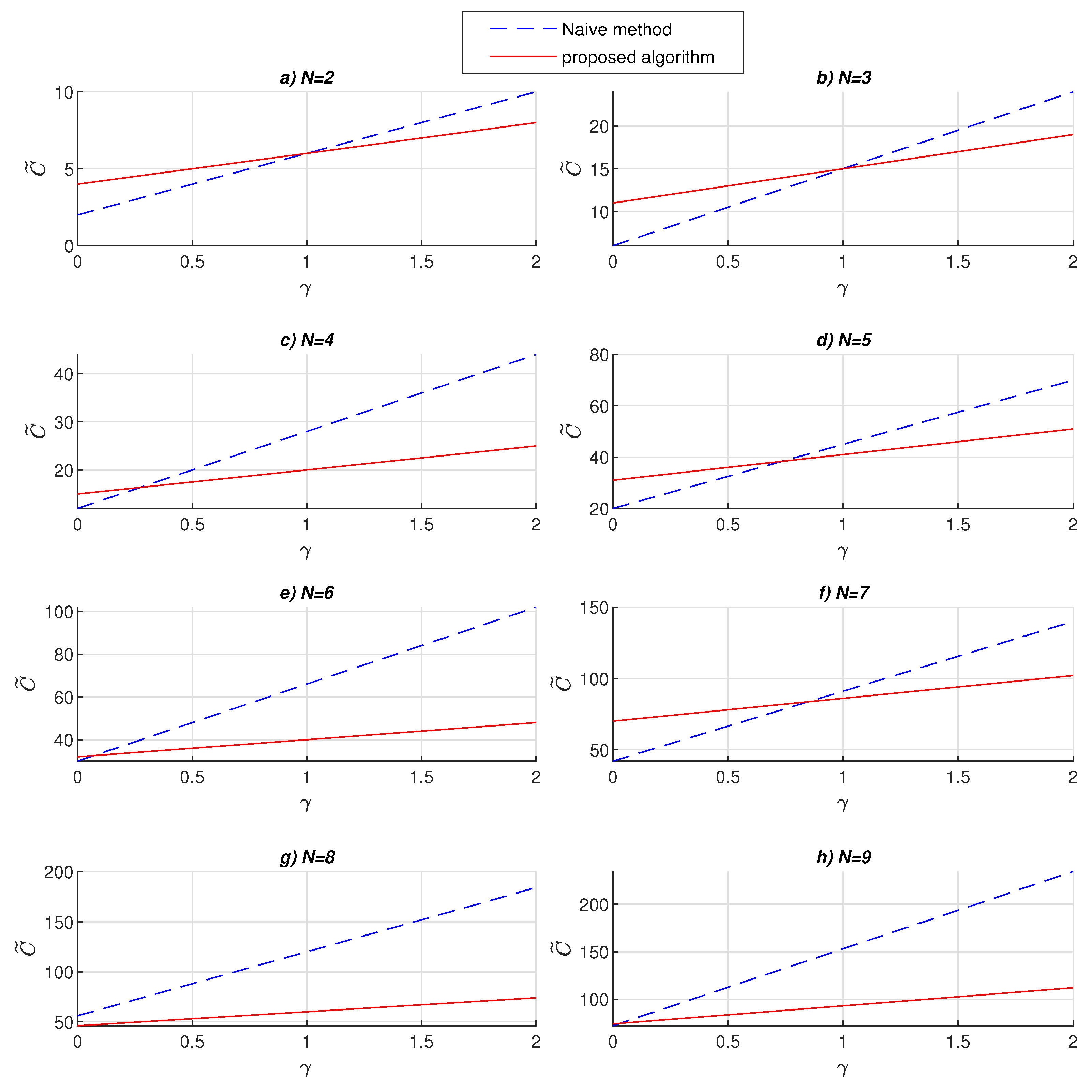
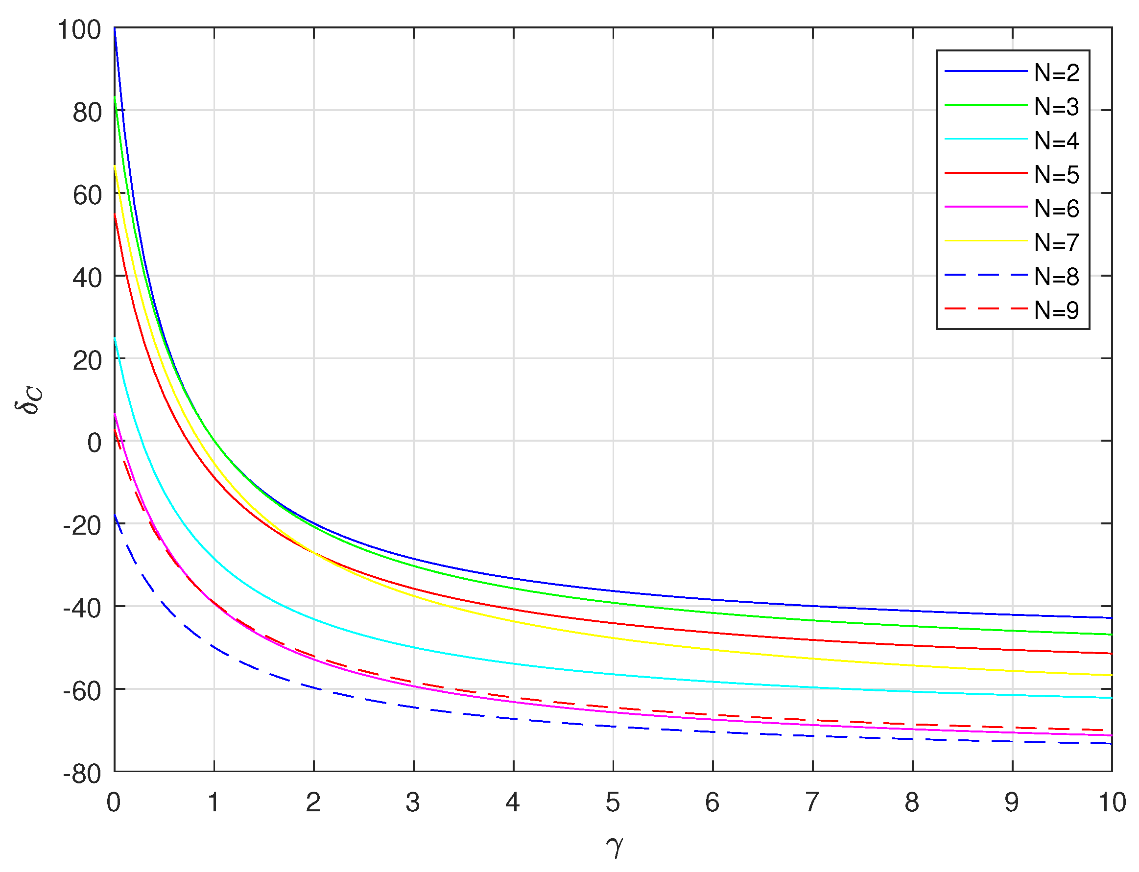
4. Implementation Complexity

We now estimate the hardware implementation costs of each solution. We assumed that the hardware implementation cost of the hardwired multiplier is $\alpha$ and the hardware implementation cost of the two-input adder is $\beta$. By the hardware implementation cost of the estimated solution, we mean a generalized assessment of the hardware complexity of implementing specific solutions, considering the area within the VLSI, the dissipation power, and therefore, the consumed energy. We also took into account that the N-input adder consists of N − 1 two-input adders. In this way, we treated the implementation cost of an N-input adder as the sum of the implementation costs of N − 1 two-input adders. Then, the total hardware implementation cost C of each solution is equal to:

$$C=\alpha M+\beta A$$

where M and A mean, respectively, the number of multipliers and the number of two-input adders required for the fully parallel implementation of a particular solution. We can normalize the above equation regarding the cost of the adder, obtaining the normalized cost:

$$\tilde{C}=\gamma M+A$$

where $\gamma =\alpha /\beta$ is the relative cost coefficient of the multiplier.

Table 1. Comparative estimates of the number of hardwired multipliers and adders for the case of completely parallel implementations of the naive-method-based solutions and of the proposed solutions.

Length N	Number of Arithmetical Blocks (Multipliers—“×” and Adders—“+”)				Implementation Normalized Cost Estimate
	Naive Method		Proposed Solutions		$\tilde{\mathit{C}}$
0	“×”	“+”	“×”	“+”	Naive Method		Proposed Solutions
2	4	2	2	4	$4\gamma +2$		$2\gamma +4$
3	9	6	4	11	$9\gamma +6$		$4\gamma +11$
4	16	12	5	15	$16\gamma +12$		$5\gamma +15$
5	25	20	10	31	$25\gamma +20$		$10\gamma +31$
6	36	30	8	32	$36\gamma +30$		$8\gamma +32$
7	49	42	16	70	$49\gamma +42$		$16\gamma +70$
8	64	56	14	46	$64\gamma +56$		$14\gamma +46$
9	81	72	19	73	$81\gamma +72$		$19\gamma +74$

shows estimates of the number of arithmetic blocks for the fully parallel implementation of the short-length circular convolution algorithms. The last two columns of the table show the unified hardware costs for the implementation of the corresponding solutions, expressed in terms of the implementation cost of one two-input adder. The charts presented in Figure 9 illustrate the normalized hardware implementation costs $\tilde{C}$ of the proposed solution and naive method for various values of $\gamma$ and N.

Cost comparisons can also be made using percentage changes:

$${\delta }_c=\frac{{\tilde{C}}_p-{\tilde{C}}_n}{{\tilde{C}}_n}100\%$$

where ${\tilde{C}}_p$ and ${\tilde{C}}_n$ are the normalized cost of proposed algorithm and naive method, respectively.

Figure 10 shows the value of percentage changes as a function of the relative cost coefficient for various values of N. Assuming that the cost of the multiplier is always at least equal to, and most often greater than, the cost of the adder $\gamma \ge 1$, the cost of the proposed algorithm is never greater than that of the naive method, and in some cases, even cost savings of over 70% are obtained.

5. Conclusions

In this article, we analyzed the possibilities of reducing the multiplicative complexity of computing circular convolutions for input sequences of small lengths. We synthesized new hardware-efficient, fully parallel algorithms to implement these operations for $N=$ 3, 4, 5, 6, 7, 8, and 9. The reduced multiplicative complexity of the proposed algorithms is especially important when developing specialized fully parallel VLSI processors, since it minimizes the number of necessary hardware multipliers and reduces the power dissipation, as well as the total cost of the implementation of the entire system being introduced [30,31,32]. Thus, a decrease in the number of multipliers, even at the expense of a moderate increase in the number of adders, plays an important role in the hardware implementation of the proposed algorithms. Consequently, the use of the proposed solutions makes it possible to reduce the complexity of the hardware implementation of the cyclic convolution kernels. In addition, as can be seen from Figure 1, Figure 2, Figure 3, Figure 4, Figure 5, Figure 6, Figure 7 and Figure 8, the algorithms presented in the article have a pronounced regular and modular structure. This facilitates the mapping of these algorithms to the ASIC structure and unifies their implementation in FPGAs. Thus, the acceleration of computations in the implementation of these algorithms can also be achieved by parallelizing the computations.

References

1. Loulou, A.; Yli-Kaakinen, J.; Renfors, M. Efficient fast-convolution based implementation of 5G waveform processing using circular convolution decomposition. In Proceedings of the 2017 IEEE International Conference on Communications (ICC), Paris, France, 21–25 May 2017; pp. 1–7. [Google Scholar]
2. Loulou, A.; Yli-Kaakinen, J.; Renfors, M. Advanced low-complexity multicarrier schemes using fast-convolution processing and circular convolution decomposition. IEEE Trans. Signal Process. 2019, 67, 2304–2319. [Google Scholar] [CrossRef]
3. Mathieu, M.; Henaff, M.; LeCun, Y. Fast training of convolutional networks through ffts. arXiv 2013, arXiv:1312.5851. [Google Scholar]
4. Lin, S.; Liu, N.; Nazemi, M.; Li, H.; Ding, C.; Wang, Y.; Pedram, M. FFT-based deep learning deployment in embedded systems. In Proceedings of the 2018 Design, Automation & Test in Europe Conference & Exhibition (DATE), Dresden, Germany, 19–23 March 2018; pp. 1045–1050. [Google Scholar]
5. Abtahi, T.; Shea, C.; Kulkarni, A.; Mohsenin, T. Accelerating convolutional neural network with fft on embedded hardware. IEEE Trans. Very Large Scale Integr. (VLSI) Syst. 2018, 26, 1737–1749. [Google Scholar] [CrossRef]
6. Burrus, S.C.; Parks, T.W. DFT/FFT and Convolution Algorithms; John Wiley & Sons: Hoboken, NJ, USA, 1985. [Google Scholar]
7. Blahut, R.E. Fast Algorithms for Signal Processing; Cambridge University Press: Cambridge, UK, 2010. [Google Scholar]
8. McClellen, J.H.; Rader, C.M. Number Theory in Digital Signal Processing; Professional Technical Reference; Prentice Hall: Hoboken, NJ, USA, 1979. [Google Scholar]
9. Tolimieri, R.; An, M.; Lu, C. Algorithms for Discrete Fourier Transform and Convolution; Springer: Berlin/Heidelberg, Germany, 1989. [Google Scholar]
10. Berg, L.; Nussbaumer, H. Fast Fourier Transform and Convolution Algorithms. Z. Angew. Math. Mech. 1982, 62, 282. [Google Scholar] [CrossRef]
11. Garg, H.K. Digital Signal Processing Algorithms: Number Theory, Convolution, Fast Fourier Transforms, and Applications; Routledge: London, UK, 2017. [Google Scholar]
12. Bi, G.; Zeng, Y. Transforms and Fast Algorithms for Signal Analysis and Representations; Springer Science & Business Media: Berlin/Heidelberg, Germany, 2003. [Google Scholar]
13. Selesnick, I.W.; Burrus, C.S. Extending Winograd’s small convolution algorithm to longer lengths. In Proceedings of the IEEE International Symposium on Circuits and Systems-ISCAS’94, London, UK, 30 May–2 June 1994; Volume 2, pp. 449–452. [Google Scholar]
14. Stasinski, R. Extending sizes of effective convolution algorithms. Electron. Lett. 1990, 26, 1602–1604. [Google Scholar] [CrossRef]
15. Karas, P.; Svoboda, D. Algorithms for efficient computation of convolution. In Design and Architectures for Digital Signal Processing; IntechOpen: London, UK, 2013; pp. 179–208. [Google Scholar]
16. Mohammad, K.; Agaian, S. Efficient FPGA implementation of convolution. In Proceedings of the 2009 IEEE International Conference on Systems, Man and Cybernetics, San Antonio, TX, USA, 11–14 October 2009; pp. 3478–3483. [Google Scholar]
17. Duhamel, P.; Vetterli, M. Cyclic convolution of real sequences: Hartley versus fourier and new schemes. In Proceedings of the ICASSP’86. IEEE International Conference on Acoustics, Speech, and Signal Processing, Tokyo, Japan, 7–11 April 1986; Volume 11, pp. 229–232. [Google Scholar]
18. Duhamel, P.; Vetterli, M. Improved Fourier and Hartley transform algorithms: Application to cyclic convolution of real data. IEEE Trans. Acoust. Speech Signal Process. 1987, 35, 818–824. [Google Scholar] [CrossRef] [Green Version]
19. Meher, P.; Panda, G. Fast Computation of Circular Convolution of Real Valued Data using Prime Factor Fast Hartley Transform Algorithm. IEEE J. Res. 1995, 41, 261–264. [Google Scholar] [CrossRef]
20. Reju, V.G.; Koh, S.N.; Soon, Y. Convolution using discrete sine and cosine transforms. IEEE Signal Process. Lett. 2007, 14, 445–448. [Google Scholar] [CrossRef]
21. Cheng, C.; Parhi, K.K. Hardware efficient fast DCT based on novel cyclic convolution structures. IEEE Trans. Signal Process. 2006, 54, 4419–4434. [Google Scholar] [CrossRef]
22. Chan, Y.H.; Siu, W.C. General approach for the realization of DCT/IDCT using convolutions. Signal Process. 1994, 37, 357–363. [Google Scholar] [CrossRef]
23. Hunt, B. A matrix theory proof of the discrete convolution theorem. IEEE Trans. Audio Electroacoust. 1971, 19, 285–288. [Google Scholar] [CrossRef]
24. Cariow, A.; Paplinski, J.P. Some algorithms for computing short-length linear convolution. Electronics 2020, 9, 2115. [Google Scholar] [CrossRef]
25. Adámek, K.; Dimoudi, S.; Giles, M.; Armour, W. GPU fast convolution via the overlap-and-save method in shared memory. ACM Trans. Archit. Code Optim. (TACO) 2020, 17, 1–20. [Google Scholar] [CrossRef]
26. Narasimha, M.J. Modified overlap-add and overlap-save convolution algorithms for real signals. IEEE Signal Process. Lett. 2006, 13, 669–671. [Google Scholar] [CrossRef]
27. Huang, T.S. Two-dimensional digital signal processing II. Transforms and median filters. In Two-Dimensional Digital Signal Processing II. Transforms and Median Filters; Topics in Applied Physics; Springer: Berlin/Heidelberg, Germany, 1981; Volume 43. [Google Scholar]
28. Parhi, K.K. VLSI Digital Signal Processing Systems: Design and Implementation; John Wiley & Sons: Hoboken, NJ, USA, 2007. [Google Scholar]
29. Ju, C.; Solomonik, E. Derivation and Analysis of Fast Bilinear Algorithms for Convolution. arXiv 2019, arXiv:1910.13367. [Google Scholar] [CrossRef]
30. Regalia, P.A.; Sanjit, M.K. Kronecker products, unitary matrices and signal processing applications. SIAM Rev. 1989, 31, 586–613. [Google Scholar] [CrossRef]
31. Granata, J.; Conner, M.; Tolimieri, R. The tensor product: A mathematical programming language for FFTs and other fast DSP operations. IEEE Signal Process. Mag. 1992, 9, 40–48. [Google Scholar] [CrossRef]
32. Saha, P.; Banerjee, A.; Dandapat, A.; Bhattacharyya, P. ASIC implementation of high speed processor for calculating discrete fourier transformation using circular convolution technique. WSEAS Trans. Circuits Syst. 2011, 10, 278–288. [Google Scholar]
Figure 1. Algorithmic structure of the processing core for the computation of the 2-point circular convolution.
Electronics 10 02800 g001
Figure 2. Algorithmic structure of the processing core for the computation of the 3-point circular convolution.
Electronics 10 02800 g002
Figure 3. Algorithmic structure of the processing core for the computation of the 4-point circular convolution.
Electronics 10 02800 g003
Figure 4. Algorithmic structure of the processing core for the computation of the 5-point circular convolution.
Electronics 10 02800 g004
Figure 5. Algorithmic structure of the processing core for the computation of the 6-point circular convolution.
Electronics 10 02800 g005
Figure 6. Algorithmic structure of the processing core for the computation of the 7-point circular convolution.
Electronics 10 02800 g006
Figure 7. Algorithmic structure of the processing core for the computation of the 8-point circular convolution.
Electronics 10 02800 g007
Figure 8. Algorithmic structure of the processing core for the computation of the 9-point circular convolution.
Electronics 10 02800 g008
Figure 9. The normalized hardware implementation costs C ˜ of the proposed solution and naive method, as a function of the relative cost coefficient γ of the multiplier, for various N.
Electronics 10 02800 g009
Figure 10. The value of percentage changes δ c as a function of the relative cost coefficient γ for various values of N.
Electronics 10 02800 g010