Article

No-Reference Video Quality Assessment Based on Benford’s Law and Perceptual Features

Ronin Institute, Montclair, NJ 07043, USA
Electronics 2021, 10(22), 2768; https://doi.org/10.3390/electronics10222768
Submission received: 26 October 2021 / Revised: 6 November 2021 / Accepted: 10 November 2021 / Published: 12 November 2021

Abstract

:
No-reference video quality assessment (NR-VQA) has piqued the scientific community’s interest throughout the last few decades, owing to its importance in human-centered interfaces. The goal of NR-VQA is to predict the perceptual quality of digital videos without any information about their distortion-free counterparts. Over the past few decades, NR-VQA has become a very popular research topic due to the spread of multimedia content and video databases. For successful video quality evaluation, creating an effective video representation from the original video is a crucial step. In this paper, we propose a powerful feature vector for NR-VQA inspired by Benford’s law. Specifically, it is demonstrated that first-digit distributions extracted from different transform domains of the video volume data are quality-aware features and can be effectively mapped onto perceptual quality scores. Extensive experiments were carried out on two large, authentically distorted VQA benchmark databases.

1. Introduction

As digital media takes a more central part in our daily lives, research on video quality assessment (VQA) becomes more and more important. For instance, about 70% of the overall Internet bandwidth is occupied by digital video streaming [1]. Moreover, it is predicted that the occupied bandwidth will increase to between 80% and 90% by 2022 [2]. As a consequence, the precise estimation of video quality is of vital importance for video streaming and sharing. In addition, VQA is also crucial in video restoration, reproduction, enhancement, and compression. Hence, the scientific community has devoted much attention and effort to this research field, continuously developing and devising algorithms, methods, and metrics that are able to estimate digital videos’ perceptual quality.
The most accurate way to assess video quality is to collect subjective opinions from human observers in a laboratory environment involving experts. This process is called subjective video quality assessment, which is rather time consuming and expensive. However, the scores collected in subjective user studies can be applied as ground-truth data for objective video quality assessment. Namely, objective video quality assessment deals with the construction of algorithms that accurately estimate the perceptual quality of a given video sequence. Depending on the availability of the reference, distortion-free videos, objective VQA methods can be grouped into three classes: full-reference (FR), reduced-reference (RR), and no-reference (NR) ones. As the names indicate, FR-VQA algorithms have full information about the reference videos, while NR-VQA ones do not have access to the reference videos. Moreover, RR-VQA methods can be considered as a transition between FR-VQA and NR-VQA algorithms. Namely, they have partial information about the reference videos, for example in the form of sets of extracted features.
In this paper, we propose a novel NR-VQA algorithm utilizing Benford’s law. Frank Benford, a physicist with General Electric, collected over 20,000 numbers in 1938 from extremely various sources, such as Readers’ Digest articles, atomic weights, population sizes, drainage rates of rivers, and physical constants [3,4]. It was demonstrated that the distribution of the first digits follows an algorithmic rule. Moreover, the observation works on a distribution of numbers if that distribution spans over a few orders of magnitude. Benford’s law states that the leading d ( d { 1 , . . . , 9 } ) in a natural dataset occurs with probability:
P ( d ) = log 10 ( d + 1 ) log 10 ( d ) = log 10 d + 1 d = log 10 1 + 1 d .
Figure 1 depicts the distribution of leading digits in natural datasets predicted by Benford’s law. Benford’s law has been proven as an efficient tool in digital analysis technology [5,6]. Namely, the first-digit distribution (FDD) in accounting data of companies and unmanipulated macroeconomic data are expected to follow Benford’s law [7,8,9]. First, Jolion [10] investigated Benford’s law in the context of digital images. The FDD pixel values do not follow Benford’s law, since pixel values are in the interval of [ 0 , 255 ] and do not span over a few magnitudes. However, the FDD of gradient magnitudes matches well with Benford’s law prediction. Similarly, Perez-Gonzalez et al. [11,12] pointed out that the discrete cosine transform (DCT) coefficients of a digital image follow Benford’s law. Fu et al. [13] demonstrated that the FDD of DCT coefficients can be used for the detection of distorted JPEG images. Similarly, Andriotis et al. [14] utilized the FDD of DCT coefficients, but they used it for image steganalysis to ascertain whether a digital image contains a hidden message or not. In our previous study [15], we demonstrated that FDDs extracted from different domains (wavelet, DCT, shearlet, singular values) are quality-aware features and they can be used for no-reference image quality assessment.

1.1. Contributions

The main contributions of this paper are the following. In our previous works [15,16], the usage of FDD feature vectors was thoroughly investigated in the context of no-reference image quality assessment. Specifically, it was proven that FDDs of different 2D transform domains are quality-aware features and can be mapped effectively onto image quality scores. In contrast, we explored the applicability of video-level FDD-based feature vectors for NR-VQA in this study. We demonstrate that quality-aware FDD feature vectors can be extracted from the video volume data considering different 3D transform domains (spatial, wavelet, discrete cosine transform, discrete Fourier transform, higher-order singular-values). It is demonstrated that fusing FDD-based and perceptual features results in a powerful video representation for NR-VQA.

1.2. Structure

The rest of the paper is organized as follows. An overview is provided about NR-VQA in Section 2. Subsequently, Section 3 contains a detailed description of the proposed method based on Benford’s law. Section 4 presents the experimental results and analysis on publicly available VQA databases. Finally, this study is concluded in Section 5.

2. Related Work

As already mentioned, VQA can be classified into two groups: subjective and objective. Specifically, subjective VQA deals with measuring perceptual video quality involving human observers either in a laboratory environment or in a crowdsourcing experiment [17,18], while objective VQA attempts to devise mathematical algorithms that are able to estimate video signals’ human perceptual quality. In the literature, one can find many recommendations for choosing video sequences, system settings, and test methodologies for subjective VQA. These are defined in the documents of the International Telecommunication Union, such as ITU-R BT.500 [19], ITU-T P.913 [20], or ITU-T P.910 [21]. The average judgment of the human observers is expressed as the mean opinion score (MOS), which can range from 1–5 or 0–100, for example. Moreover, a higher MOS indicates higher visual quality. As a result of subjective VQA experiments, many VQA databases are publicly available for researchers, such as KoNViD-1k [22] or the LIVE Video Quality Challenge (VQC) [23] database. An overview of publicly available benchmark VQA databases can be found in [24,25,26].
In the literature, objective NR-VQA algorithms are classified into bitstream-based, pixel-based, and hybrid models [27]. Bitstream-based algorithms extract features directly from encoded video sequences to predict perceptual video quality. For example, Argyropoulos et al. [28] presented an algorithm for the prediction of continuous estimates of the visibility of packet losses. Moreover, the authors demonstrated that visible losses have a significant impact on video quality degradation. Keimel et al. [29] devised a H.264/AVC bitstream algorithm. Namely, multiple features were extracted from the encoded video sequences, such as slice type, bits per slice, average quantization parameter per slice, average, minimum and maximum motion vector length per slice, and average and maximum motion vector error per slice. These features were mapped onto perceptual quality scores using partial least squares regression. Similarly, Chen and Wu [30] identified a set of features, such as concealment error, motion vector concealment error, pixel-level transmission distortion, etc., and conclude from them the perceptual video quality. The approach of Pandremmenou et al. [31] is also similar to the method of Argyropoulos et al. [28], but they defined a wider range of features. Specifically, a feature vector of length 46 was mapped onto perceptual quality scores using the least absolute shrinkage and selection operator regression. In contrast to bitstream-based methods, pixel-based algorithms utilize the raw video signal solely as the input. For example, Saad et al. [32] extracted features using the 3D-DCT. Then, a linear kernel support vector regressor (SVR) was trained to predict the visual quality of videos. Similarly, Zhu et al. [33] presented a DCT-based NR-VQA model. Specifically, frame-level DCT coefficient-based features (peakiness, smoothness, sharpness, etc.) were temporally pooled to compile video-level feature vectors. Next, the video-level feature vectors were mapped onto perceptual quality scores using a shallow neural network. In contrast, Dendi et al. [34] constructed a video representation using the mean subtracted and contrast normalized (MSCN) coefficients of certain spatiotemporal statistics of a natural video. More specifically, an asymmetric generalized Gaussian distribution was fit onto the MSCN coefficients of a natural video and its Gabor bandpass filtered counterpart. The parameters of asymmetric generalized Gaussian distributions were considered as quality-aware features and mapped onto perceptual quality scores with the help of an SVR. Ebenezer et al. [35] proposed a video representation that contains information about both the spatial and temporal information. Namely, the authors defined space–time chips as quality-aware features, which are cuts from the original video data in specific directions obtained from local motion flow. Subsequently, asymmetric generalized Gaussian distributions were fit to the bandpass histograms of space–time chips. Finally, the parameters of asymmetric generalized Gaussian distributions were mapped onto perceptual quality scores by a trained SVR.
Recently, deep-learning techniques have been proven very successful in image-based object detection [36], semantic segmentation [37], image generation [38], etc. Researchers also have introduced deep-learning-based NR-VQA methods. For instance, Li et al. [39] extracted quality-aware visual features from video blocks using a 3D shearlet transform. These features were fed into convolutional neural networks to predict perceptual video quality. Ahn and Lee [40] combined deep and hand-crafted features for NR-VQA. Specifically, a pretrained convolutional neural network was applied to extract features from video frames, while temporal features were modeled by hand-crafted features. Li et al. [41] introduced a mixed dataset training strategy. Namely, the authors’ network was trained on mixed data and addressed by two different loss functions, i.e., monotonicity-induced and linearity-induced losses.

3. Proposed Method

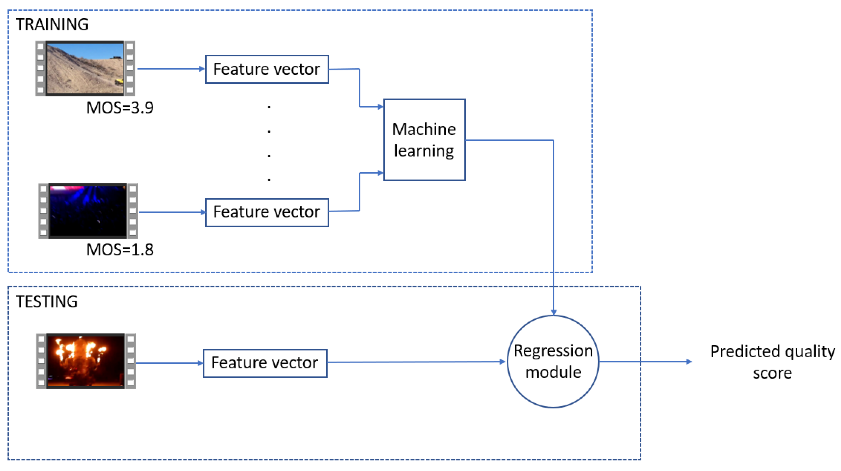
The high-level overview of the introduced NR-VQA algorithm is depicted in Figure 2. As can be seen from this figure, video-level feature vectors are extracted from the training video sequences to train a machine-learning model, which is later utilized in the testing stage to estimate the perceptual quality of unseen videos. In this paper, a novel set of FDD and perceptual quality-aware features are presented for NR-VQA. Section 3.1 describes the proposed FDD-based features, while the applied perceptual features are described in Section 3.2.

3.1. FDD-Based Features

FDD features are extracted from the spatial, 3D wavelet, 3D Fourier, and 3D discrete cosine transform domains of a video sequence. Moreover, the FDD of higher-order singular-values of a video sequence is also considered as a quality-aware feature.
FDDs are extracted in the spatial domain of video sequences using 3D directional gradients. To find the directional gradients of a 3D grayscale video sequence of size N 1 × N 2 × N 3 , the 3D extension of the Sobel edge detector [42] (illustrated in Figure 3) was applied in this paper. Moreover, the size of the applied 3D Sobel operator for each direction was 3 × 3 × 3 . The convolution operators in the x, y, and z directions are given as:
S x ( : , : , 1 ) = 1 0 1 3 0 3 1 0 1 , S x ( : , : , 0 ) = 3 0 3 6 0 6 3 0 3 , S x ( : , : , 1 ) = 1 0 1 3 0 3 1 0 1 ,
S y ( : , : , 1 ) = 1 3 1 0 0 0 1 3 1 , S y ( : , : , 0 ) = 3 6 3 0 0 0 3 6 3 , S y ( : , : , 1 ) = 1 3 1 0 0 0 1 3 1 ,
S z ( : , : , 1 ) = 1 3 1 3 6 3 1 3 1 , S z ( : , : , 0 ) = 0 0 0 0 0 0 0 0 0 , S z ( : , : , 1 ) = 1 3 1 3 6 3 1 3 1 .
If we define V as the grayscale video sequence of size N 1 × N 2 × N 3 , and G x , G y , and G z are three arrays, which at each point consist of the x, y, and z directional derivative approximations, the computations are as follows:
G x = S x V , G y = S y V , and G z = S z V ,
where * stands for the 3D convolution operator. In Figure 3, the 3D Sobel operators and filtering are depicted where the x, y, and z axes correspond to the crossline, inline, and time axes of a grayscale video sequence, respectively. In the spatial domain, three FDDs are obtained from G x , G y , and G z .
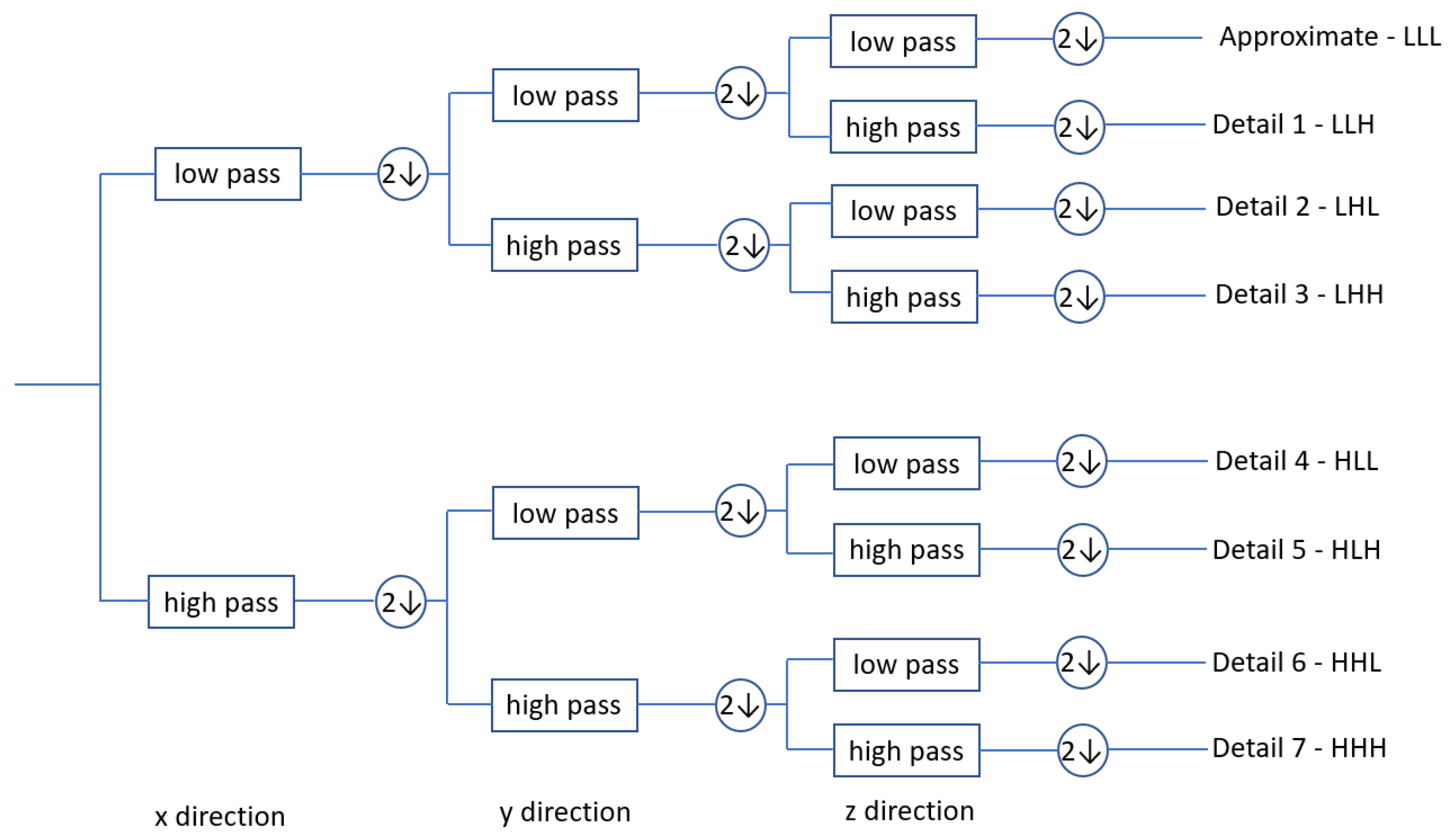
Discrete wavelet transform (DWT) was devised to correct the resolution problems of the short-time discrete Fourier transform [43]. It has a huge number of applications in engineering and computer science, since it is able to represent signals in a redundant form. The 3D DWT is depicted in Figure 4. As one can see from this figure, the volume data (in our case, a grayscale video sequence) are decomposed into eight sub-bands in the case of single-level processing. These can be grouped into three distinct classes: an approximation sub-band ( L L L ) , spectral variation sub-bands ( L L H , L H H , H L H ) , and spatial variation sub-bands ( L H L , H L L , H H L ) . Moreover, Daubechies mother wavelets were utilized in our implementation. Quality-aware FDD features were extracted from the spectral variation and the spatial variation sub-bands.
The 3D DCT is an extension of the DCT to the three-dimensional space and defined as:
X k 1 , k 2 , k 3 = n 1 = 0 N 1 1 n 2 = 0 N 2 1 n 3 = 0 N 3 1 V n 1 , n 2 , n 3 cos π N 1 n 1 + 1 2 k 1 cos π N 2 n 2 + 1 2 k 2 cos π N 3 n 3 + 1 2 k 3 , for k i = 0 , 1 , 2 , , N i 1 , i = 1 , 2 , 3
where X k 1 , k 2 , k 3 are the 3D DCT coefficients and V n 1 , n 2 , n 3 denote the n 1 th, n 2 th, and n 3 th pixel value of the grayscale video sequence V . The FDDs of 3D DCT coefficients are considered as quality-aware features.
Besides 3D DCT coefficients, 3D discrete Fourier transform (DFT) coefficients of grayscale video sequences were also used to extract an FDD feature vector for video representation. The DFT of a grayscale video sequence V (three-dimensional array of size N 1 × N 2 × N 3 ) is defined as:
Y k 1 , k 2 , k 3 = n 1 = 0 N 1 1 ω m 1 k 1 , n 1 n 2 = 0 N 2 1 ω m 2 k 2 , n 2 n 3 = 0 N 3 1 ω m 3 k 3 , n 3 V n 1 , n 2 , n 3 ,
where Y k 1 , k 2 , k 3 stand for the DFT coefficients, V n 1 , n 2 , n 3 denote the n 1 th, n 2 th, and n 3 th pixel value of the grayscale video sequence V , ω m k = e 2 π i m k ( m k = 1 , 2 , 3 ) are the complex roots of unity, and i is the imaginary unit. In our implementation, DFT coefficients were determined by the fast Fourier transform [44]. In our study, the FFD of DFT coefficients were used as quality-aware features.
Higher-order singular-value decomposition (HOSVD) can be considered as one generalization of matrix singular-value decomposition [45]. Namely, a tensor’s HOSVD corresponds to a specific orthogonal Tucker decomposition [46,47]. Every tensor V of size N 1 × N 2 × N 3 can be written as:
V = n 1 = 1 N 1 n 2 = 1 N 2 n 3 = 1 N 3 σ n 1 , n 2 , n 3 ( u n 1 ( 1 ) u n 2 ( 2 ) u n 3 ( 3 ) ) ,
where ∘ stands for the outer product operation and:
U ( 1 ) = [ u 1 ( 1 ) , u 2 ( 1 ) , . . . , u N 1 ( 1 ) ] ,
U ( 2 ) = [ u 1 ( 2 ) , u 2 ( 2 ) , . . . , u N 2 ( 2 ) ] ,
U ( 3 ) = [ u 1 ( 3 ) , u 2 ( 3 ) , . . . , u N 3 ( 3 ) ] ,
are three unitary matrices of sizes N 1 × N 1 , N 2 × N 2 , N 3 × N 3 , respectively. The FDD of singular values ( σ n 1 , n 2 , n 3 ’s) was used as the quality-aware feature.
In Table 1, Table 2, Table 3, Table 4, Table 5, Table 6 and Table 7, the mean FDDs of X directional gradient magnitudes, Y directional gradient magnitudes, HLL wavelet coefficients, HHL wavelet coefficients, 3D DFT coefficients, 3D DCT coefficients, and higher-order singular-values are summarized with respect to five equal MOS intervals of KoNViD-1k [22]. In KoNViD-1k [22], the lowest possible video quality is represented by M O S = 1.0 , while M O S = 5.0 stands for the highest possible video quality. It can be observed that the FDDs of videos with a higher quality fit better the prediction of Benford’s law. Moreover, the distance between the actual FDD and the Benford law prediction is also lower in the case of high-quality videos. The distance is given using the symmetric Kullback–Leibler (sKL) divergence.

3.2. Perceptual Features

In our model, several perceptual features were also incorporated, which are consistent with human quality judgments [48]. Moreover, a subset of the presented perceptual features was also applied for no-reference image quality assessment in our previous work [16]:
1.
Blur: This is the shape and area in an image that cannot be seen clearly because no distinct outline is present or an object is moving fast. Artifacts generated by blur usually result in the loss of details. Hereby, the amount of blur in an image heavily influences humans’ quality perception. Due its low computational costs, we adopted the approach of Crété-Roffet et al. [49] to quantify the amount of blur in an image, which is based on the comparison between variations of adjacent pixels after low-pass filtering;
2.
Colorfulness: There are more studies that suggest colorfulness as an important factor for human visual quality perception [48,50,51]. In our study, Hasler and Suesstrunk’s model [52] was applied to measure colorfulness. Let’ us denote with R, G, and B the red, green, and blue channels of an RGB image, respectively. Two matrices are derived for the color channels: r g = R G and y b = 1 2 ( R + G ) B . Next, colorfulness ( C F ) is defined as:
C F = σ r g 2 + σ y b 2 + 3 10 μ r g 2 + μ y b 2 ,
where σ 2 and μ stand for the variance and mean of their respective matrices. A video sequence’s colorfulness is considered as the average value of individual frames’ colorfulness;
3.
Contrast: Perceptual image quality is strongly influenced by contrast, since humans’ ability to distinguish objects from each other in an image heavily depends on it [53]. In [16], Matkovic et al.’s [54] global contrast factor (GCF) model was applied to quantify image contrast. However, GCF’s computational cost is large, which makes it not feasible to measure a video sequence’s contrast. That is why we adopted here the root-mean-squared (RMS) contrast for measuring the contrast of a video frame. RMS contrast is defined as the standard deviation of the pixel intensities [55]:
C R M S = 1 M · N i = 0 N 1 j = 0 M 1 ( I i , j I ¯ ) 2 ,
where I i , j stands for the ith, jth pixel intensity of a 2D grayscale image I with size M × N . A video sequence’s contrast is considered as the average value of the video frames’ contrast;
4.
Dark channel feature: He et al. [56] investigated the properties of fog-free natural images. It was found that dark pixels are those pixels whose intensity values are close to zero at least in one color channel within an image patch [57]. Based on this, a dark channel is defined as:
I d a r k ( x ) = min y Ω ( x ) ( min c { R , G , B } I c ( y ) ) ,
where I c ( y ) denotes the intensity of a color channel (R, G, or B) and Ω ( x ) is an image patch centered on x. Based on the above definition, the dark channel feature ( D C F ) of an image is given as:
D C F = 1 | | S | | i S I d a r k ( i ) c { R , G , B } I c ( i ) ,
where S stands for the area of the input image. A video sequence’s D C F is considered as the average value of the individual video frames’ D C F ;
5.
Entropy: The entropy of a digital image is a feature that gives information about the average content in an image. The concept of the entropy of a signal in general is very old. Namely, it comes from Shannon’s theory of communication [58]. The entropy of a 2D grayscale image is given as:
E I = n p ( n ) · log 2 p ( n ) ,
where p ( n ) stands for the empirical distribution of grayscale values in image I. The entropy of a video sequence is defined as the average of the video frames’ entropy;
6.
Mean of phase congruency: Phase congruency (PC) characterizes a digital image in the frequency domain. Phase congruency is given by the following equation:
P C 1 ( x ) = | E ( x ) | n A n ( x ) ,
where E ( x ) corresponds to the energy of signal x and can be given as:
E ( x ) = | X ( j ω ) | 2
where X ( j ω ) is the Fourier transform of signal x and A n ( x ) denotes the nth Fourier amplitude of signal x. To incorporate noise compensation, Kovesi [59] modified the above definition of PC by adding weights for the frequency spread:
P C 2 ( x ) = n W ( x ) A n ( x ) Δ ϕ n ( x ) T n A n ( x ) + ϵ ,
where W ( x ) is the weight function of the frequency spread, · stands for the floor function, T is an estimation of the noise level, and ϵ is a small constant to avoid division by zero. Moreover, ϕ n ( x ) denotes the nth Fourier component at x and can be expressed as:
Δ ϕ n ( x ) = c o s ( ϕ n ( x ) ϕ n ( x ) ¯ ) | s i n ( ϕ n ( x ) ϕ n ( x ) ¯ ) | ,
where ϕ n ( x ) ¯ is the average phase at x. For a video sequence, the video frames’ mean PC values are averaged to obtain a perceptual feature;
7.
Spatial information: The gradient magnitude maps of each video frame were determined with the help of a Sobel filter, and the standard deviations of each Sobel map were taken. The spatial information ( S I ) of a video sequence is the average of the Sobel maps’ standard deviations;
8.
Temporal information: This characterizes the amount of temporal changes in a given video sequence [21]. In this study, the temporal information ( T I ) of a video sequence was considered as the mean of the pixelwise frame differences’ standard deviations;
9.
Natural image quality evaluator (NIQE): The NIQE [60] measures the distance between the natural scene statistics-based features extracted from an image and certain ideal features. In the case of the NIQE, the features are modeled as multidimensional Gaussian distributions. Specifically, the value given by the NIQE can be considered as the degree of deviation from naturalness of a digital image. In this study, the naturalness of a video sequence is characterized by the average of the video frames’ NIQE values.
The average values of the above-described perceptual features with respect to five equal MOS intervals of KoNViD-1k [22] are given in Table 8. It can be observed that they are roughly proportional to the quality classes. With a properly chosen regression module, they can be good predictors of perceptual video quality.

4. Experimental Results and Analysis

In this section, our experimental results and analysis are presented. First, the applied benchmark VQA database is described in Section 4.1. Second, the evaluation metrics are given in Section 4.2. Third, the evaluation environment and implementation details are specified in Section 4.3. Fourth, a parameter study related to the proposed method is presented in Section 4.4 to reason about the design choices. Finally, a comparison to other state-of-the-art methods is presented in Section 4.5.

4.1. Databases

In our study, the KoNViD-1k [22] and LIVE VQC [23] benchmark VQA databases were used to carry out experiments and compare the proposed method to the state-of-the-art.
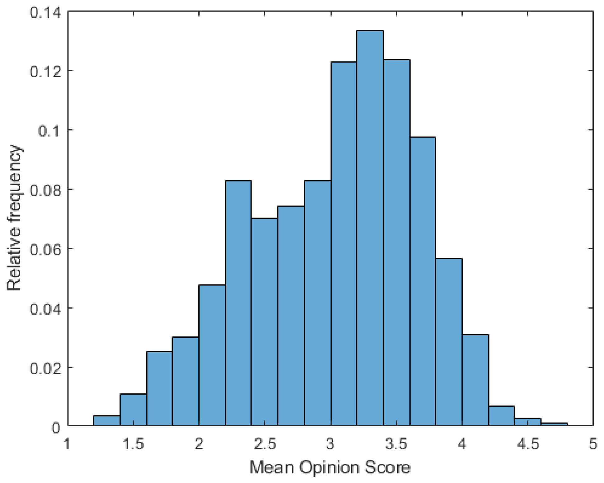
The videos of KoNViD-1k [22] were collected from the YFCC100M [61] database with respect to six predefined attributes: blur amount, colorfulness, contrast, spatial information, temporal information, and the natural image quality evaluator [60]. MOS values for each video were collected through a crowdsourcing process [62]. In this crowdsourcing process, 642 crowd workers from 64 countries participated, and they produced at least 50 judgments per video. In KoNViD-1k [22], M O S = 1.0 represents the lowest possible perceptual video quality, while M O S = 5.0 stands for the highest possible quality. The main characteristics of KoNViD-1k [22] are summarized in Table 9. The empirical distribution of the MOS values in KoNViD-1k [22] is depicted in Figure 5.
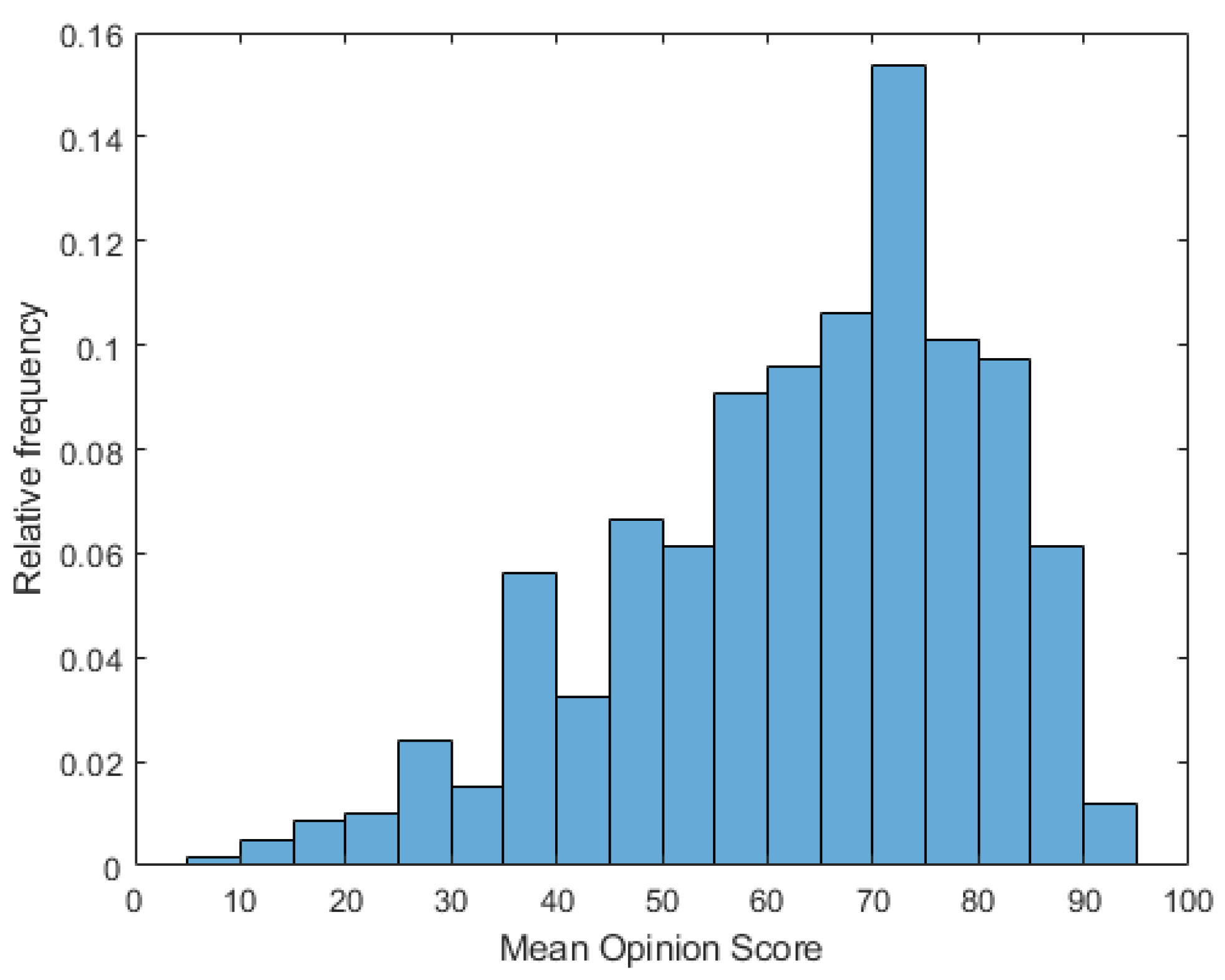
Similar to KoNViD-1k [22], LIVE VQC [23] contains authentically distorted video sequences with their corresponding perceptual quality scores. Specifically, it consists of 585 unique videos captured by 101 different video devices (mainly by smartphones). Moreover, the average length of the videos is 10 s. Similar to KoNViD-1k [22], the subjective quality scores were obtained in a crowdsourcing experiment where 4776 unique observers produced more than 205,000 opinion scores. The main characteristics of LIVE VQC [23] are summarized in Table 9. The empirical distribution of the MOS values in LIVE VQC [23] is depicted in Figure 6.

4.2. Evaluation Metrics

Similar to image quality assessment, the evaluation and performance ranking of NR-VQA algorithms rely on the measurement of the correlation between predicted and ground-truth perceptual quality scores. To this end, Pearson’s linear correlation coefficient (PLCC) and Spearman’s rank-order correlation coefficient (SROCC) are widely applied in the literature [26]. The PLCC between the ground-truth and predicted quality scores can be defined as:
P L C C ( x , y ) = i = 1 N ( x i x ¯ ) ( y i y ¯ ) i = 1 N ( x i x ¯ ) 2 i = 1 N ( y i y ¯ ) 2 ,
where N is the length of vectors x and y , x i and y i are the ith elements of vectors x and y , and finally, x ¯ and y ¯ stand for the mean of vectors x and y . According to the recommendations of the Video Quality Expert Group [63], we adjusted the scaling and nonlinearity effect between the predicted and ground-truth scores by an f ( x ) nonlinear transform, which is given by:
f ( x ) = τ 1 τ 2 1 + e x τ 3 | τ 4 | + τ 2 ,
where τ 1 , τ 2 , τ 3 , and τ 4 are the fitting parameters. In contrast to the PLCC, the SROCC characterizes the monotonic relationship between the predicted and ground-truth quality scores and can be defined as:
S R O C C ( x , y ) = 1 6 i = 1 N d i 2 N ( N 2 1 ) ,
where:
d i = r a n k ( x i ) r a n k ( y i ) .
In this study, we report on the median values of the PLCC and SROCC after 1000 random training–testing splits.

4.3. Evaluation Environment and Implementation Details

To evaluate the proposed and the other state-of-the-art methods, KoNViD-1k [22] and LIVE VQC [23] were divided randomly into a training ( 80 % ) and a test set ( 20 % ) . As already mentioned, the median PLCC and SROCC values are reported in this study, which were measured over 1000 random train–test splits. The computer configuration applied in our experiments is summarized in Table 10. Moreover, the proposed methods were implemented in MATLAB R2021a.

4.4. Parameter Study

In this subsection, a parameter study is presented. Specifically, the performance of different FDD and perceptual features was examined with different regression modules, such as the SVR with linear and radial basis functions (RBFs), Gaussian process regression (GPR) with a rational quadratic kernel function, binary tree regression (BTR), and random forest regression (RFR). The results are summarized in Table 11. From these results, it can be clearly observed that the FDD features exhibited a rather weak or mediocre correlation with the ground-truth quality scores on KoNViD-1k [22], while considering all FDDs showed a rather strong correlation. In addition to this, the perceptual features also exhibited a strong correlation with the ground-truth quality scores on KoNViD-1k [22]. By fusing the FDDs and perceptual features together, a powerful feature vector can be obtained, which outperformed both the FDDs and perceptual features. Furthermore, GPR with a rational quadratic kernel function was the best-performing regression module, since it provided the highest correlation values almost in all cases. Based on these observations, we propose two NR-VQA methods, i.e., FDD-VQA and FDD + Perceptual-VQA, which are compared to the state-of-the-art in the next subsection. FDD-VQA considers only the FDD-based feature vectors, while FDD + Perceptual-VQA fuses FDDs and perceptual features together. Both proposed methods rely on GPRs with rational quadratic kernel functions as the regression modules.

4.5. Comparison to the State-of-the-Art

In this subsection, several NR-VQA methods, such as NVIE [64], V.BLIINDS [32], VIIDEO [65], 3D-MSCN [34], ST-Gabor [34], and 3D-MSCN + ST-Gabor [34], whose original source codes were made publicly available by the authors, are compared to the proposed FDD-VQA and FDD + Perceptual-VQA methods. These methods were evaluated exactly the same way as the proposed methods (described in Section 4.2). Moreover, the performance metrics of other state-of-the-art algorithms (FC model [66], STFC model [66], STS-SVR [67], STS-MLP [67], ChipQA [35]) were collected from the corresponding research studies.
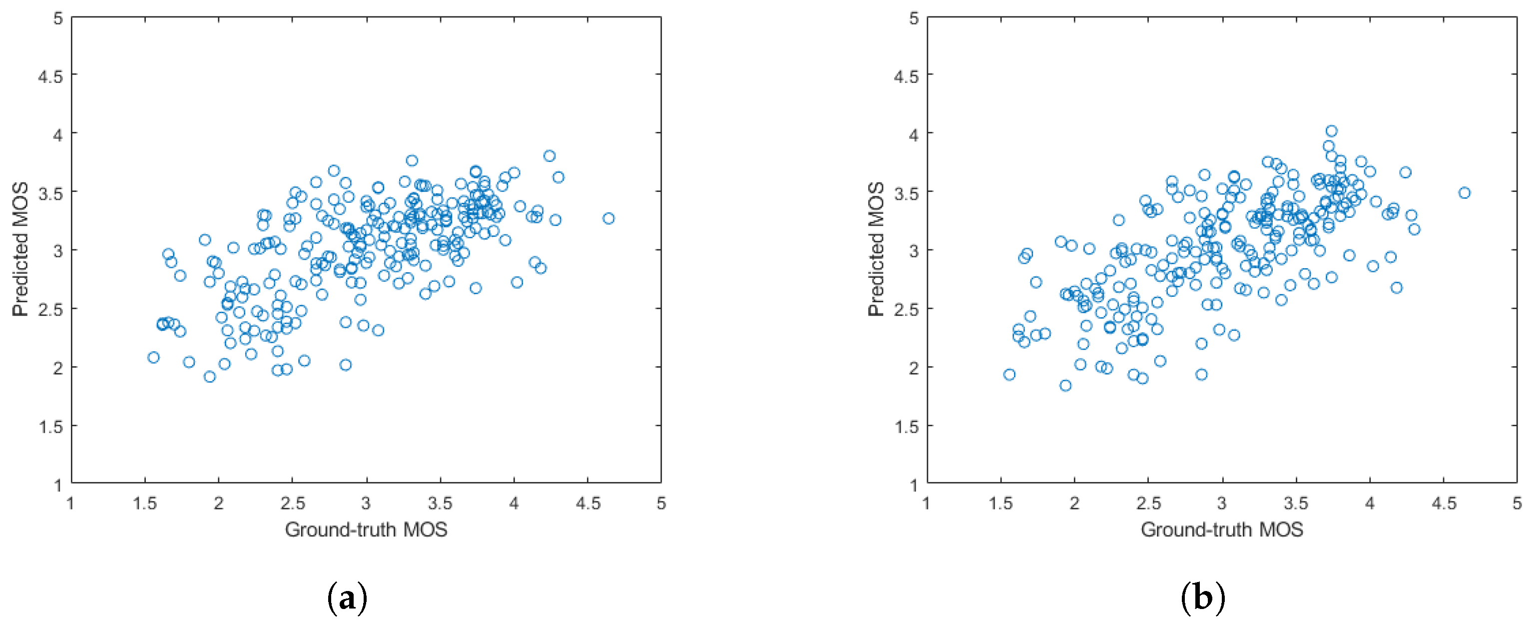
The results for KoNViD-1k [22] are summarized in Table 12. It is clear from this table that the proposed NR-VQA approaches were able to provide competitive performance on a large, challenging VQA database both in terms of the PLCC and SROCC. Specifically, FDD-VQA, which solely relies on FDD feature vectors extracted from different domains (spatial, wavelet, Fourier, DCT, HOSVD), was able to outperform nine methods out of the examined eleven ones, while FDD + Perceptual-VQA outperformed all the considered state-of-the-art algorithms by a large margin. Figure 7 illustrates the scatter plots of the ground-truth MOS values against the predicted MOS values on the KoNViD-1k [22] test set.
The results for LIVE VQC [23] are summarized in Table 13. It can be seen that the proposed FDD-VQA and FDD + Perceptual-VQA methods were able to reach or outperform the state-of-the-art on LIVE VQC [23]. Specifically, FDD + Perceptual-VQA outperformed all the other examined NR-VQA algorithms, while FDD-VQA was able to reach the performance of the state-of-the-art.
To prove the significance of the presented results, one-sided t-tests were carried out on the 1000 SROCC values using a 95 % confidence level. The results measured on KoNViD-1k are summarized in Table 14. From these results, it can be seen that the performance of FDD + Perceptual-VQA was statistically significantly better than those of the other examined state-of-the-art methods. Similarly, the results for LIVE VQC [23] are summed up in Table 15. It can be observed that the proposed FDD + Perceptual-VQA was statistically better than the other considered state-of-the-art methods except for V.BLIINDS [32], where no difference is exhibited.

5. Conclusions

In this paper, we proposed a novel NR-VQA algorithm based on a set of novel quality-aware features, which relies on the FDDs of different domains (spatial, wavelet, DCT, DFT, HOSVD) and perceptual features. Specifically, we analyzed different FDD-based feature vectors in detail for NR-VQA. To this end, a detailed parameter study was established with respect to different domains and regression modules. It was demonstrated that state-of-the-art performance can be achieved in NR-VQA by considering only FDDs from different domains. Moreover, it was pointed out that fusing FDD and perceptual feature vectors together resulted in a powerful video representation for NR-VQA, which was able to outperform the state-of-the-art on two large authentically distorted VQA benchmark databases. Finally, the significance of the presented results was statistically proven with one-sided t-tests. Future work involves a real-time implementation of FDD feature extraction for NR-VQA on graphical processing units since many transformations and histogram calculations can be accelerated with them.
To facilitate the reproducibility of the presented results, the source code of the proposed method written in MATLAB R2021a is available at: https://github.com/Skythianos/Benford-VQA, accessed on 11 November 2021.

Funding

This research received no external funding.

Institutional Review Board Statement

Not applicable.

Informed Consent Statement

Not applicable.

Data Availability Statement

The datasets used were obtained from public open-source datasets from: 1. KoNViD-1k: http://database.mmsp-kn.de/konvid-1k-database.html (accessed on 11 November 2021); 2. LIVE VQC: https://live.ece.utexas.edu/research/LIVEVQC/index.html (accessed on 11 November 2021).

Acknowledgments

We thank the anonymous reviewers for their careful reading of our manuscript and their many insightful comments and suggestions.

Conflicts of Interest

The author declares no conflict of interest.

Abbreviations

The following abbreviations are used in this manuscript:
3Dthree-dimensional
BTRbinary tree regression
Ccontrast
CFcolorfulness
DCFdark channel feature
DCTdiscrete cosine transform
DFTdiscrete Fourier transform
DSLRdigital single-lens reflex
DWTdiscrete wavelet transform
FDDfirst-digit distribution
FRfull-reference
FR-VQAfull-reference video quality assessment
GCFglobal contrast factor
GPRGaussian process regression
HOSVDhigher-order singular-value decomposition
JPEGJoint Photographic Experts Group
LIVELaboratory for Image and Video Engineering
MOSmean opinion score
MPEGMoving Picture Experts Group
MSCNmean subtracted and contrast normalized
NIQEnatural image quality evaluator
NRno-reference
NR-VQAno-reference video quality assessment
PCphase congruency
PLCCPearson’s linear correlation coefficient
RBFradial basis function
RFRrandom forest regression
RMSroot mean square
RRreduced-reference
RR-VQAreduced-reference video quality assessment
SIspatial information
SROCCSpearman’s rank-order correlation coefficient
SVRsupport vector regressor
TItemporal information
VQAvideo quality assessment
VQCvideo quality challenge
YFCC100MYahoo Flickr Creative Commons 100 Million

References

  1. Index, C.V.N. Cisco visual networking index: Forecast and methodology 2015–2020. In White Paper; CISCO: San Jose, CA, USA, 2015. [Google Scholar]
  2. Forecast, G. Cisco visual networking index: Global mobile data traffic forecast update, 2017–2022. Update 2019, 2017, 2022. [Google Scholar]
  3. Benford, F. The law of anomalous numbers. Proc. Am. Philos. Soc. 1938, 78, 551–572. [Google Scholar]
  4. Fewster, R.M. A simple explanation of Benford’s Law. Am. Stat. 2009, 63, 26–32. [Google Scholar] [CrossRef] [Green Version]
  5. Özer, G.; Babacan, B. Benford’s Law and Digital Analysis: Application on Turkish Banking Sector. Bus. Econ. Res. J. 2013, 4, 29–41. [Google Scholar] [CrossRef] [Green Version]
  6. Hüllemann, S.; Schüpfer, G.; Mauch, J. Application of Benford’s law: A valuable tool for detecting scientific papers with fabricated data? Der Anaesthesist 2017, 66, 795–802. [Google Scholar] [CrossRef] [PubMed]
  7. Nye, J.; Moul, C. The political economy of numbers: On the application of Benford’s law to international macroeconomic statistics. BE J. Macroecon. 2007, 7, 1–14. [Google Scholar] [CrossRef]
  8. Gonzalez-Garcia, M.J.; Pastor, M.G.C. Benford’s Law and Macroeconomic Data Quality; International Monetary Fund: Washington, DC, USA, 2009. [Google Scholar]
  9. Rauch, B.; Göttsche, M.; Brähler, G.; Kronfeld, T. Deficit versus social statistics: Empirical evidence for the effectiveness of Benford’s law. Appl. Econ. Lett. 2014, 21, 147–151. [Google Scholar] [CrossRef]
  10. Jolion, J.M. Images and Benford’s law. J. Math. Imaging Vis. 2001, 14, 73–81. [Google Scholar]
  11. Pérez-González, F.; Heileman, G.L.; Abdallah, C.T. A generalization of Benford’s law and its application to images. In Proceedings of the 2007 European Control Conference (ECC), Kos, Greece, 2–5 July 2007; pp. 3613–3619. [Google Scholar]
  12. Pérez-González, F.; Heileman, G.L.; Abdallah, C.T. Benford’s law in image processing. In Proceedings of the 2007 IEEE International Conference on Image Processing, San Antonio, TX, USA, 16–19 September 2007; Volume 1, pp. 405–408. [Google Scholar]
  13. Fu, D.; Shi, Y.Q.; Su, W. A generalized Benford’s law for JPEG coefficients and its applications in image forensics. In Security, Steganography, and Watermarking of Multimedia Contents IX; International Society for Optics and Photonics: Bellingham, WA, USA, 2007; Volume 6505, p. 65051L. [Google Scholar]
  14. Andriotis, P.; Oikonomou, G.; Tryfonas, T. JPEG steganography detection with Benford’s Law. Digit. Investig. 2013, 9, 246–257. [Google Scholar] [CrossRef]
  15. Varga, D. Analysis of Benford’s Law for No-Reference Quality Assessment of Natural, Screen-Content, and Synthetic Images. Electronics 2021, 10, 2378. [Google Scholar] [CrossRef]
  16. Varga, D. No-reference image quality assessment based on the fusion of statistical and perceptual features. J. Imaging 2020, 6, 75. [Google Scholar] [CrossRef]
  17. Hosu, V.; Lin, H.; Saupe, D. Expertise screening in crowdsourcing image quality. In Proceedings of the 2018 Tenth International Conference on Quality of Multimedia Experience (QoMEX), Sardinia, Italy, 29–31 May 2018; pp. 1–6. [Google Scholar]
  18. Hoßfeld, T.; Keimel, C.; Hirth, M.; Gardlo, B.; Habigt, J.; Diepold, K.; Tran-Gia, P. Best practices for QoE crowdtesting: QoE assessment with crowdsourcing. IEEE Trans. Multimed. 2013, 16, 541–558. [Google Scholar] [CrossRef]
  19. ITU-R. Methodology for the Subjective Assessment of the Quality of Television Pictures; Recommendation ITU-R BT; International Telecommunication Union: Geneva, Switzerland, 2012; pp. 500–513. [Google Scholar]
  20. International Telecommunication Union. Methods for the Subjective Assessment of Video Quality Audio Quality and Audiovisual Quality of Internet Video and Distribution Quality Television in Any Environment; Series P: Terminals And Subjective and Objective Assessment Methods; International Telecommunication Union: Geneva, Switzerland, 2016. [Google Scholar]
  21. ITU-T RECOMMENDATION. Subjective Video Quality Assessment Methods for Multimedia Applications; International Telecommunication Union: Geneva, Switzerland, 1999. [Google Scholar]
  22. Hosu, V.; Hahn, F.; Jenadeleh, M.; Lin, H.; Men, H.; Szirányi, T.; Li, S.; Saupe, D. The Konstanz natural video database (KoNViD-1k). In Proceedings of the 2017 Ninth International Conference on Quality of Multimedia Experience (QoMEX), Erfurt, Germany, 29 May–2 June 2017; pp. 1–6. [Google Scholar]
  23. Sinno, Z.; Bovik, A.C. Large-scale study of perceptual video quality. IEEE Trans. Image Process. 2018, 28, 612–627. [Google Scholar] [CrossRef] [Green Version]
  24. Winkler, S. Analysis of public image and video databases for quality assessment. IEEE J. Sel. Top. Signal Process. 2012, 6, 616–625. [Google Scholar] [CrossRef]
  25. Okarma, K. Image and video quality assessment with the use of various verification databases. In Proceedings of the New Electrical and Electronic Technologies and their Industrial Implementation, Zakopane, Poland, 18–21 June 2013; Volume 142. [Google Scholar]
  26. Xu, L.; Lin, W.; Kuo, C.C.J. Visual Quality Assessment by Machine Learning; Springer: Berlin/Heidelberg, Germany, 2015. [Google Scholar]
  27. Winkler, S.; Mohandas, P. The evolution of video quality measurement: From PSNR to hybrid metrics. IEEE Trans. Broadcast. 2008, 54, 660–668. [Google Scholar] [CrossRef]
  28. Argyropoulos, S.; Raake, A.; Garcia, M.N.; List, P. No-reference video quality assessment for SD and HD H. 264/AVC sequences based on continuous estimates of packet loss visibility. In Proceedings of the 2011 Third International Workshop on Quality of Multimedia Experience, Mechelen, Belgium, 7–9 September 2011; pp. 31–36. [Google Scholar]
  29. Keimel, C.; Habigt, J.; Klimpke, M.; Diepold, K. Design of no-reference video quality metrics with multiway partial least squares regression. In Proceedings of the 2011 Third International Workshop on Quality of Multimedia Experience, Mechelen, Belgium, 7–9 September 2011; pp. 49–54. [Google Scholar]
  30. Chen, Z.; Wu, D. Prediction of transmission distortion for wireless video communication: Analysis. IEEE Trans. Image Process. 2011, 21, 1123–1137. [Google Scholar] [CrossRef]
  31. Pandremmenou, K.; Shahid, M.; Kondi, L.P.; Lövström, B. A no-reference bitstream-based perceptual model for video quality estimation of videos affected by coding artifacts and packet losses. In Human Vision and Electronic Imaging XX; International Society for Optics and Photonics: Bellingham, WA, USA, 2015; Volume 9394, p. 93941F. [Google Scholar]
  32. Saad, M.A.; Bovik, A.C.; Charrier, C. Blind prediction of natural video quality. IEEE Trans. Image Process. 2014, 23, 1352–1365. [Google Scholar] [CrossRef] [PubMed] [Green Version]
  33. Zhu, K.; Li, C.; Asari, V.; Saupe, D. No-reference video quality assessment based on artifact measurement and statistical analysis. IEEE Trans. Circuits Syst. Video Technol. 2014, 25, 533–546. [Google Scholar] [CrossRef] [Green Version]
  34. Dendi, S.V.R.; Channappayya, S.S. No-reference video quality assessment using natural spatiotemporal scene statistics. IEEE Trans. Image Process. 2020, 29, 5612–5624. [Google Scholar] [CrossRef]
  35. Ebenezer, J.P.; Shang, Z.; Wu, Y.; Wei, H.; Bovik, A.C. No-reference video quality assessment using space-time chips. In Proceedings of the 2020 IEEE 22nd International Workshop on Multimedia Signal Processing (MMSP), Tampere, Finland, 21–24 September 2020; pp. 1–6. [Google Scholar]
  36. Girshick, R. Fast r-cnn. In Proceedings of the IEEE International Conference on Computer Vision, Santiago, Chile, 11–18 December 2015; pp. 1440–1448. [Google Scholar]
  37. Long, J.; Shelhamer, E.; Darrell, T. Fully convolutional networks for semantic segmentation. In Proceedings of the IEEE Conference on Computer Vision and Pattern Recognition, Boston, MA, USA, 7–12 June 2015; pp. 3431–3440. [Google Scholar]
  38. Ren, Y.; Yu, X.; Chen, J.; Li, T.H.; Li, G. Deep image spatial transformation for person image generation. In Proceedings of the IEEE/CVF Conference on Computer Vision and Pattern Recognition, Seattle, WA, USA, 13–19 June 2020; pp. 7690–7699. [Google Scholar]
  39. Li, Y.; Po, L.M.; Cheung, C.H.; Xu, X.; Feng, L.; Yuan, F.; Cheung, K.W. No-reference video quality assessment with 3D shearlet transform and convolutional neural networks. IEEE Trans. Circuits Syst. Video Technol. 2015, 26, 1044–1057. [Google Scholar] [CrossRef]
  40. Ahn, S.; Lee, S. Deep blind video quality assessment based on temporal human perception. In Proceedings of the 2018 25th IEEE International Conference on Image Processing (ICIP), Athens, Greece, 7–10 October 2018; pp. 619–623. [Google Scholar]
  41. Li, D.; Jiang, T.; Jiang, M. Unified quality assessment of in-the-wild videos with mixed datasets training. Int. J. Comput. Vis. 2021, 129, 1238–1257. [Google Scholar] [CrossRef]
  42. Aqrawi, A.A.; Boe, T.H.; Barros, S. Detecting salt domes using a dip guided 3D Sobel seismic attribute. In SEG Technical Program Expanded Abstracts 2011; Society of Exploration Geophysicists: Tulsa, OK, USA, 2011; pp. 1014–1018. [Google Scholar]
  43. Weeks, M.; Bayoumi, M. 3D discrete wavelet transform architectures. In Proceedings of the 1998 IEEE International Symposium on Circuits and Systems (Cat. No. 98CH36187), ISCAS’98, Monterey, CA, USA, 31 May–3 June 1998; Volume 4, pp. 57–60. [Google Scholar]
  44. Heideman, M.T.; Johnson, D.H.; Burrus, C.S. Gauss and the history of the fast Fourier transform. Arch. Hist. Exact Sci. 1985, 34, 265–277. [Google Scholar] [CrossRef] [Green Version]
  45. Baranyi, P.; Varlaki, P.; Szeidl, L.; Yam, Y. Definition of the HOSVD based canonical form of polytopic dynamic models. In Proceedings of the 2006 IEEE International Conference on Mechatronics, Budapest, Hungary, 3–5 July 2006; pp. 660–665. [Google Scholar]
  46. Tucker, L.R. The extension of factor analysis to three-dimensional matrices. Contrib. Math. Psychol. 1964, 110119. [Google Scholar]
  47. De Lathauwer, L.; De Moor, B.; Vandewalle, J. A multilinear singular value decomposition. SIAM J. Matrix Anal. Appl. 2000, 21, 1253–1278. [Google Scholar] [CrossRef] [Green Version]
  48. Jenadeleh, M. Blind Image and Video Quality Assessment. Ph.D. Thesis, University of Konstanz, Konstanz, Germany, 2018. [Google Scholar]
  49. Crete, F.; Dolmiere, T.; Ladret, P.; Nicolas, M. The blur effect: Perception and estimation with a new no-reference perceptual blur metric. In Human Vision and Electronic Imaging XII; International Society for Optics and Photonics: Bellingham, WA, USA, 2007; Volume 6492, p. 64920I. [Google Scholar]
  50. de Ridder, H. Naturalness and image quality: Saturation and lightness variation in color images of natural scenes. J. Imaging Sci. Technol. 1996, 40, 487–493. [Google Scholar]
  51. Palus, H. Colorfulness of the image: Definition, computation, and properties. In Lightmetry and Light and Optics in Biomedicine 2004; International Society for Optics and Photonics: Bellingham, WA, USA, 2006; Volume 6158, p. 615805. [Google Scholar]
  52. Hasler, D.; Suesstrunk, S.E. Measuring colorfulness in natural images. In Human Vision and Electronic Imaging VIII; International Society for Optics and Photonics: Bellingham, WA, USA, 2003; Volume 5007, pp. 87–95. [Google Scholar]
  53. Segler, D.; Pettitt, G.; van Kessel, P. The importance of contrast and its effect on image quality. SMPTE Motion Imaging J. 2002, 111, 533–540. [Google Scholar] [CrossRef]
  54. Matkovic, K.; Neumann, L.; Neumann, A.; Psik, T.; Purgathofer, W. Global Contrast Factor-a New Approach to Image Contrast; The Eurographics Association: Geneve, Switzerland, 2005; pp. 159–167. [Google Scholar]
  55. Peli, E. Contrast in complex images. JOSA A 1990, 7, 2032–2040. [Google Scholar] [CrossRef]
  56. He, K.; Sun, J.; Tang, X. Single image haze removal using dark channel prior. IEEE Trans. Pattern Anal. Mach. Intell. 2010, 33, 2341–2353. [Google Scholar]
  57. Lee, S.; Yun, S.; Nam, J.H.; Won, C.S.; Jung, S.W. A review on dark channel prior based image dehazing algorithms. EURASIP J. Image Video Process. 2016, 2016, 1–23. [Google Scholar] [CrossRef] [Green Version]
  58. Shannon, C.E. A mathematical theory of communication. Bell Syst. Tech. J. 1948, 27, 379–423. [Google Scholar] [CrossRef] [Green Version]
  59. Kovesi, P. Phase congruency detects corners and edges. In Proceedings of the Australian Pattern Recognition Society Conference, DICTA, Sydney, Australia, 10–12 December 2003; Volume 2003. [Google Scholar]
  60. Mittal, A.; Soundararajan, R.; Bovik, A.C. Making a “completely blind” image quality analyzer. IEEE Signal Process. Lett. 2012, 20, 209–212. [Google Scholar] [CrossRef]
  61. Thomee, B.; Shamma, D.A.; Friedland, G.; Elizalde, B.; Ni, K.; Poland, D.; Borth, D.; Li, L.J. YFCC100M: The new data in multimedia research. Commun. ACM 2016, 59, 64–73. [Google Scholar] [CrossRef]
  62. Saupe, D.; Hahn, F.; Hosu, V.; Zingman, I.; Rana, M.; Li, S. Crowd workers proven useful: A comparative study of subjective video quality assessment. In Proceedings of the 8th International Conference on Quality of Multimedia Experience, QoMEX 2016, Lisbon, Portugal, 6–8 June 2016. [Google Scholar]
  63. Rohaly, A.M.; Corriveau, P.J.; Libert, J.M.; Webster, A.A.; Baroncini, V.; Beerends, J.; Blin, J.L.; Contin, L.; Hamada, T.; Harrison, D.; et al. Video quality experts group: Current results and future directions. In Visual Communications and Image Processing 2000; International Society for Optics and Photonics: Bellingham, WA, USA, 2000; Volume 4067, pp. 742–753. [Google Scholar]
  64. Mittal, A. Natural Scene Statistics-Based Blind Visual Quality Assessment in the Spatial Domain. Ph.D. Thesis, The University of Texas at Austin, Austin, TX, USA, 2013. [Google Scholar]
  65. Mittal, A.; Saad, M.A.; Bovik, A.C. A completely blind video integrity oracle. IEEE Trans. Image Process. 2015, 25, 289–300. [Google Scholar] [CrossRef] [PubMed]
  66. Men, H.; Lin, H.; Saupe, D. Spatiotemporal feature combination model for no-reference video quality assessment. In Proceedings of the 2018 Tenth international conference on quality of multimedia experience (QoMEX), Sardinia, Italy, 29–31 May 2018; pp. 1–3. [Google Scholar]
  67. Yan, P.; Mou, X. No-reference video quality assessment based on perceptual features extracted from multi-directional video spatiotemporal slices images. In Optoelectronic Imaging and Multimedia Technology V; International Society for Optics and Photonics: Bellingham, WA, USA, 2018; Volume 10817, p. 108171D. [Google Scholar]
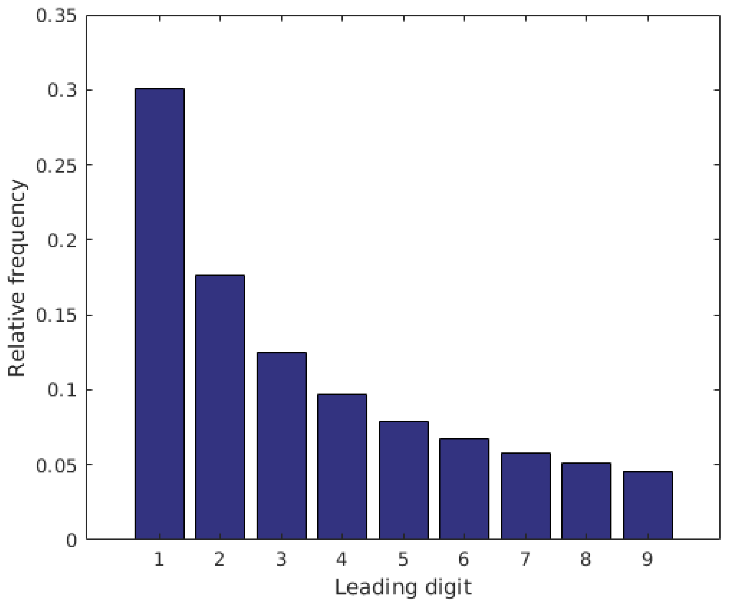
Figure 1. Illustration of Benford’s law.
Electronics 10 02768 g001
Figure 2. High-level overview of the proposed method. Video-level feature vectors are extracted from the training videos to train a machine-learning model, which is later utilized in the testing phase to predict the quality of previously unseen videos. In this study, we propose the fusion of the Benford-law-inspired first-digit distribution and perceptual features.
Electronics 10 02768 g002
Figure 3. Illustration of 3D Sobel filtering. The x, y, and z axes correspond to the crossline, inline, and time axes of a grayscale video sequence, respectively.
Electronics 10 02768 g003
Figure 4. Illustration of the 3D DWT.
Electronics 10 02768 g004
Figure 5. MOS distribution in KoNViD-1k [22].
Electronics 10 02768 g005
Figure 6. MOS distribution in LIVE VQC [23].
Electronics 10 02768 g006
Figure 7. Scatter plots of the ground-truth MOS against the predicted MOS of the proposed methods on the KoNViD-1k [22] test set. (a) FDD-VQA. (b) FDD + Perceptual-VQA.
Electronics 10 02768 g007
Table 1. Mean FDD of X directional gradient magnitudes in KoNViD-1k [22] with respect to different MOS intervals. In KoNViD-1k [22], the lowest possible video quality is represented by M O S = 1.0 , while M O S = 5.0 stands for the highest possible video quality. In the last column, the symmetric Kullback–Leibler ( s K L ) divergences between the actual FDD and the Benford law distribution are given.
123456789 s K L
4.2 M O S 5 0.3090.1830.1210.0960.0930.0590.0520.0460.0410.004
3.4 M O S < 4.2 0.3130.1800.1210.0990.0890.0590.0500.0460.0430.004
2.6 M O S < 3.4 0.3160.1800.1210.0990.0900.0580.0490.0450.0430.004
1.8 M O S < 2.6 0.3220.1770.1180.0980.0960.0560.0460.0430.0430.008
1 M O S < 1.8 0.3310.1730.1140.0980.1020.0540.0430.0420.0440.014
Benford’s law0.3010.1760.1250.0970.0790.0670.0580.0510.0460
Table 2. Mean FDD of Y directional gradient magnitudes in KoNViD-1k [22] with respect to different MOS intervals. In KoNViD-1k [22], the lowest possible video quality is represented by M O S = 1.0 , while M O S = 5.0 stands for the highest possible video quality. In the last column, the symmetric Kullback–Leibler ( s K L ) divergences between the actual FDD and the Benford law distribution are given.
123456789 s K L
4.2 M O S 5 0.3080.1840.1190.0960.0960.0590.0520.0460.0410.005
3.4 M O S < 4.2 0.3080.1860.1200.0980.0920.0590.0500.0450.0420.005
2.6 M O S < 3.4 0.3130.1830.1200.0980.0930.0580.0480.0440.0420.006
1.8 M O S < 2.6 0.3220.1780.1160.0970.1010.0550.0460.0420.0420.011
1 M O S < 1.8 0.3280.1730.1130.0980.1080.0530.0440.0410.0430.016
Benford’s law0.3010.1760.1250.0970.0790.0670.0580.0510.0460
Table 3. Mean FDD of HLL wavelet coefficients in KoNViD-1k [22] with respect to different MOS intervals. In KoNViD-1k [22], the lowest possible video quality is represented by M O S = 1.0 , while M O S = 5.0 stands for the highest possible video quality. In the last column, the symmetric Kullback–Leibler ( s K L ) divergences between the actual FDD and the Benford law distribution are given.
123456789 s K L
4.2 M O S 5 0.2940.1870.1520.0770.0400.0440.1420.0330.0320.097
3.4 M O S < 4.2 0.3060.1560.1860.0680.0450.0460.1390.0290.0260.114
2.6 M O S < 3.4 0.3060.1540.1930.0660.0390.0450.1460.0270.0240.139
1.8 M O S < 2.6 0.2890.1570.1980.0700.0380.0530.1500.0250.0200.148
1 M O S < 1.8 0.2800.1580.2000.0770.0360.0590.1490.0230.0160.156
Benford’s law0.3010.1760.1250.0970.0790.0670.0580.0510.0460
Table 4. Mean FDD of HHL wavelet coefficients in KoNViD-1k [22] with respect to different MOS intervals. In KoNViD-1k [22], the lowest possible video quality is represented by M O S = 1.0 , while M O S = 5.0 stands for the highest possible video quality. In the last column, the symmetric Kullback–Leibler ( s K L ) divergences between the actual FDD and the Benford law distribution are given.
123456789 s K L
4.2 M O S 5 0.2660.1440.1960.0670.0560.0330.1840.0390.0170.191
3.4 M O S < 4.2 0.2570.1340.2590.0660.0520.0300.1580.0320.0120.233
2.6 M O S < 3.4 0.2430.1270.2880.0650.0480.0300.1610.0320.0110.281
1.8 M O S < 2.6 0.2440.1120.3120.0510.0480.0270.1570.0400.0090.327
1 M O S < 1.8 0.2350.0990.3370.0460.0480.0280.1540.0440.0090.370
Benford’s law0.3010.1760.1250.0970.0790.0670.0580.0510.0460
Table 5. Mean FDD of 3D DFT coefficients in KoNViD-1k [22] with respect to different MOS intervals. In KoNViD-1k [22], the lowest possible video quality is represented by M O S = 1.0 , while M O S = 5.0 stands for the highest possible video quality. In the last column, the symmetric Kullback–Leibler ( s K L ) divergences between the actual FDD and the Benford law distribution are given.
123456789 s K L
4.2 M O S 5 0.3060.1700.1200.0950.0790.0690.0600.0530.048 6.18 × 10 4
3.4 M O S < 4.2 0.3020.1730.1230.0970.0800.0680.0590.0520.047 9.88 × 10 5
2.6 M O S < 3.4 0.2940.1720.1250.1000.0820.0690.0600.0520.046 4.45 × 10 4
1.8 M O S < 2.6 0.2880.1720.1280.1020.0840.0700.0600.0520.0450.001
1 M O S < 1.8 0.2870.1770.1310.1020.0830.0680.0580.0500.0440.0011
Benford’s law0.3010.1760.1250.0970.0790.0670.0580.0510.0460
Table 6. Mean FDD of 3D DCT coefficients in KoNViD-1k [22] with respect to different MOS intervals. In KoNViD-1k [22], the lowest possible video quality is represented by M O S = 1.0 , while M O S = 5.0 stands for the highest possible video quality. In the last column, the symmetric Kullback–Leibler ( s K L ) divergences between the actual FDD and the Benford law distribution are given.
123456789 s K L
4.2 M O S 5 0.3050.1740.1230.0960.0790.0670.0590.0520.047 1.41 × 10 4
3.4 M O S < 4.2 0.3020.1750.1240.0970.0790.0670.0590.0520.046 2.92 × 10 5
2.6 M O S < 3.4 0.2980.1740.1250.0980.0810.0680.0590.0520.046 1.03 × 10 4
1.8 M O S < 2.6 0.2950.1740.1260.0990.0810.0690.0590.0520.046 2.42 × 10 4
1 M O S < 1.8 0.2940.1760.1280.1000.0810.0680.0580.0510.045 2.77 × 10 4
Benford’s law0.3010.1760.1250.0970.0790.0670.0580.0510.0460
Table 7. Mean FDD of higher-order singular values in KoNViD-1k [22] with respect to different MOS intervals. In KoNViD-1k [22], the lowest possible video quality is represented by M O S = 1.0 , while M O S = 5.0 stands for the highest possible video quality. In the last column, the symmetric Kullback–Leibler ( s K L ) divergences between the actual FDD and the Benford law distribution are given.
123456789 s K L
4.2 M O S 5 0.3030.1750.1240.0960.0790.0670.0580.0520.046 2.75 × 10 5
3.4 M O S < 4.2 0.3000.1740.1250.0970.0800.0680.0590.0520.046 3.76 × 10 5
2.6 M O S < 3.4 0.2970.1740.1250.0980.0810.0680.0590.0520.046 1.02 × 10 4
1.8 M O S < 2.6 0.2950.1750.1250.0980.0810.0680.0580.0510.045 2.07 × 10 4
1 M O S < 1.8 0.2950.1770.1280.0990.0810.0680.0580.0510.045 2.05 × 10 4
Benford’s law0.3010.1760.1250.0970.0790.0670.0580.0510.0460
Table 8. Mean of the perceptual features in KoNViD-1k [22] with respect to different MOS intervals. In KoNViD-1k [22], the lowest possible video quality is represented by M O S = 1.0 , while M O S = 5.0 stands for the highest possible video quality.
BlurCFContrastDCFEntropyPCSITINIQE
4.2 M O S 5 0.3090.2290.2110.1977.0270.01983.4780.0343.745
3.4 M O S < 4.2 0.3710.1960.2230.2447.1030.01770.8500.0673.802
2.6 M O S < 3.4 0.4230.1930.2260.2236.8000.01359.3060.0814.163
1.8 M O S < 2.6 0.4580.1980.1880.1536.2600.00742.0720.0774.888
1 M O S < 1.8 0.4510.2130.1580.0985.5770.00734.0560.0815.356
Table 9. Overview of the KoNViD-1k [22] and LIVE VQC [23] publicly available VQA databases.
AttributeKoNViD-1k [22]LIVE VQC [23]
Year20172018
No. of sequences1200585
No. of scenes1200585
No. of devicesN/A101
Device typesDSLRsmartphone
Distortion typeauthenticauthentic
Duration∼8 s∼10 s
Resolution 960 × 540 320 × 240 1920 × 1080
Frame rate30N/A
FormatMPEG-4N/A
Rating per video50200
MOS range1.0–5.00.0–100.0
Table 10. Computer configuration applied in our experiments.
Computer modelSTRIX Z270H Gaming
CPUIntel(R) Core(TM) i7-7700K CPU 4.20 GHz (8 cores)
Memory15 GB
GPUNvidia GeForce GTX 1080
Table 11. Performance comparison of the FDD and perceptual feature vectors on KoNViD-1k [22]. Median SROCC values were measured over 1000 random train–test splits on KoNViD-1k [22].
Feature VectorLinear SVRRBF-SVRGPRBTRRFR
FDD of X directional gradient magnitudes0.4020.4190.4320.2230.218
FDD of Y directional gradient magnitudes0.4360.4090.4860.2130.238
FDD of Z directional gradient magnitudes0.3940.3590.3860.2060.183
FDD of HLL wavelet coefficients0.3200.3020.3470.1520.171
FDD of LHL wavelet coefficients0.2790.3820.4120.2010.202
FDD of HHL wavelet coefficients0.4250.4930.5030.3230.328
FDD of LLH wavelet coefficients0.3380.3870.4140.2200.237
FDD of HLH wavelet coefficients0.3470.3940.4210.2370.250
FDD of LHH wavelet coefficients0.3160.4120.4280.2290.246
FDD of HHH wavelet coefficients0.4490.4790.4980.3230.304
FDD of 3D DFT coefficients0.1360.2180.2030.0920.090
FDD of 3D DCT coefficients0.1350.1900.2070.1320.092
FDD of higher-order singular values0.1560.1170.1440.0970.091
Perceptual features0.6260.6750.6860.4880.502
All FDDs0.6170.5880.6400.3630.401
All FDDs + Perceptual0.6760.6610.7110.4720.52
Table 12. Comparison of FDD-VQA and FDD + Perceptual-VQA to the state-of-the-art on KoNViD-1k [22]. Median PLCC and SROCC values were measured over 1000 random train–test splits. The best results are in bold, while the second best results are underlined.
MethodPLCCSROCC
NVIE [64]0.4040.333
V.BLIINDS [32]0.6610.694
VIIDEO [65]0.3010.299
3D-MSCN [34]0.4010.370
ST-Gabor [34]0.6390.628
3D-MSCN + ST-Gabor [34]0.6530.640
FC Model [66]0.4920.472
STFC Model [66]0.6390.606
STS-SVR [67]0.6800.673
STS-MLP [67]0.4070.420
ChipQA [35]0.6970.694
FDD-VQA0.6540.640
FDD + Perceptual-VQA0.7160.711
Table 13. Comparison of FDD-VQA and FDD + Perceptual-VQA to the state-of-the-art on LIVE VQC [23]. Median PLCC and SROCC values were measured over 1000 random train–test splits. The best results are in bold, while the second best results are underlined. We denote by “-” when the data are not available.
MethodPLCCSROCC
NVIE [64]0.4470.459
V.BLIINDS [32]0.6900.703
VIIDEO [65]−0.006−0.034
3D-MSCN [34]0.5020.510
ST-Gabor [34]0.5910.599
3D-MSCN + ST-Gabor [34]0.6750.677
FC Model [66]--
STFC Model [66]--
STS-SVR [67]--
STS-MLP [67]--
ChipQA [35]0.6690.697
FDD-VQA0.6230.630
FDD + Perceptual-VQA0.6940.705
Table 14. A one-sided t-test was carried among 1000 SROCC values measured on KoNViD-1k [22] using a 95 % confidence level. In this table, “1” (“−1”) denotes that the row algorithm is statistically better (worse) than the column algorithm.
NVIEV.BLIINDSVIIDEO3D-MSCNST-Gabor3D-MSCN + ST-GaborFDD + Perceptual-VQA
NVIE- 1 1 1 1 1 1
V.BLIINDS1-1111 1
VIIDEO 1 1 - 1 1 1 1
3D-MSCN1 1 1- 1 1 1
ST-Gabor1 1 11- 1 1
3D-MSCN + ST-Gabor1 1 111- 1
FDD + Perceptual-VQA111111-
Table 15. A one-sided t-test was carried among 1000 SROCC values measured on LIVE VQC [23] using a 95 % confidence level. In this table, “1” (“−1”) denotes that the row algorithm is statistically better (worse) than the column algorithm, and “0” stands for no statistical difference between the algorithms.
NVIEV.BLIINDSVIIDEO3D-MSCNST-Gabor3D-MSCN + ST-GaborFDD + Perceptual-VQA
NVIE- 1 1 1 1 1 1
V.BLIINDS1-11110
VIIDEO 1 1 - 1 1 1 1
3D-MSCN111- 1 1 1
ST-Gabor1 1 11- 1 1
3D-MSCN + ST-Gabor1 1 111- 1
FDD + Perceptual-VQA101111-
Publisher’s Note: MDPI stays neutral with regard to jurisdictional claims in published maps and institutional affiliations.