Abstract
For the battery pack’s limited remaining power, two energy-aware ecological driving problems are discussed. A real-time energy-aware ecological driving control strategy is proposed to optimize energy consumption and meet the ECO driving demand. First, the vehicle longitudinal driving dynamics model and energy consumption model are established. Then, the optimal control problem is constructed with the maximum driving distance and the shortest driving time as the objective functions, respectively. With the multinomial Radau pseudo-spectral method, the optimization results of residual power, vehicle speed, and acceleration are obtained. The results show that in the case of in-vehicle driving the remaining power of the battery pack can be sensed in real-time, and the driving of intelligent electric vehicles can be planned in real-time to realize the most ecological driving with the largest driving distance and shortest driving time. The energy consumptions of vehicles, traveling at the same distance, are compared. The consumption obtained through optimization, is 26% less than the consumption of the vehicle that has not been optimized. The results show that the optimization process has certain advantages. In the future, as one of intelligent vehicles’ autonomous driving control strategies, the results have guiding and practical significance.
1. Introduction
Intelligent vehicles can provide safer, more energy-efficient, more environmentally friendly, and convenient travel modes and comprehensive solutions for common problems. Advancing intelligent vehicles has become an internationally recognized direction and focuses on future development [1]. In recent years, it is focused on the eco-driving strategy of intelligent electric vehicles [2]. For example, Fredette D et al. studied the influence of road conditions and vehicle driving parameters on eco-driving strategies and presented dynamic eco-driving’s fuel saving potential [3]. J. Wang, et al. presented the fuel consumption model for conventional diesel buses [4]. Shankar R et al. proposed an optimal energy control strategy for plug-in hybrid electric vehicles [5]. Barth M et al. proposed a dynamic ecological driving speed planning algorithm, and they found that vehicle energy consumption was the lowest when the vehicle controlled the speed with the maximum acceleration within the restricted range through the simulation analysis [6]. The applied Legendre pseudo-spectral method aims to solve engine torque and gear’s optimal control during vehicle running and applies its method to the intersection scene [7]. For the optimal control of intelligent energy-saving vehicles, L Guo et al. applied Pontriagin’s minimum value theorem combined with model predictive control, and proposed a predictive economic cruise that applied to the intersection scene. It integrated the dynamics of surrounding vehicles and the road’s information ahead for the optimal control of intelligent energy-saving vehicles [8].
With the number of hybrid electric and pure electric vehicles increasing in recent years, research has been carried out on the onboard battery group’s limited energy. Many achievements were presented on energy management and optimization of hybrid electric or pure electric vehicles [9,10,11]. To reduce the charging waiting time of pure electric vehicles, L. Gan et al. studied the speed and acceleration controller of two-wheeled electric vehicles based on energy perception [12]. On the other hand, Qin H. and Zhang W. studied the distribution of charging time between electric vehicle networks and charging stations [13].
Although much research has been conducted on the energy perception of hybrid electric vehicles (HEVs) and pure electric vehicles (EVs), there are few studies on driving control for energy management due to the complexity between vehicle dynamic characteristics and energy consumption. Based on the condition of departure, destination and travel time, and traction, Sun B et al. presented an eco-driving dynamic planning method to find an optimal speed track to reduce energy consumption [14]. Based on the dynamic planning method, Dib W et al. obtained the optimal speed tracks of pure electric vehicles to minimize the energy consumption problem [15]. The literature translates the minimization of energy consumption into optimal control. The two-point boundary value problem is obtained by Hamiltonian analysis, and the closed-loop solution is obtained based on the inverse method. Assuming that the road slope is constant and ignoring the effects of air resistance, the closed-loop solution of the two-point boundary value problem is obtained through Hamiltonian analysis.
For transforming the problem of minimizing energy consumption into an optimal control problem, Petit N et al. obtained the two-point boundary value by Hamiltonian analysis, and the closed-loop solution is obtained based on the inverse method [16]. A similar problem is studied in the literature [17]. Assuming that the road slope is constant and the influence of air resistance is ignored, the closed-loop solution of the two-point boundary value problem is obtained through Hamiltonian analysis. The literature’s mathematical model of pure electric vehicle energy consumption established the complex relationship among speed, acceleration, and energy consumption rate [18].
The analysis shows that the above achievements are obtained assuming that the battery pack has sufficient charge or that the remaining charge is not known. The battery pack’s storage power is limited and lessens with the vehicle running on the road. It is crucial to obtain the amount of charge (or remaining charge) stored in the battery pack. The remaining charge in the battery pack may or may not be sufficient for the travel task. Additionally, there is little research on intelligent electric vehicles’ ecological driving when the remaining charge of the battery pack is known. The strong constraint conditions and intelligent planning algorithms under a complex environment are of great significance and interest to research.
The proposed model [18] responds to the relationship between electric energy consumption and vehicles’ index. How to optimize energy consumption through traffic control research provides a train of thought. Based on the above methods, the optimal driving control pattern is pro-posed through efficient using of the battery’s remaining power, achieving energy awareness, the significant ecological driving control and the shortest driving time. The Radau pseudo-spectral method is used to solve the energy awareness ecological optimal control problem using the theoretical analysis for the electric vehicle longitudinal motion dynamics model. It also uses the consumed power model, the corresponding boundary constraints analysis, and the tectonic energy awareness ecological model of the optimal control problem.
The contributions of this paper are: (1) The problem of real-time energy aware ecological driving control of intelligent electric vehicles is introduced. (2) The problem of realizing the maximum driving distance and the shortest time ecological driving control of energy perception is proposed. (3) The power consumption model of the intelligent electric vehicle is established. (4) The optimal control problem model of energy perception ecological driving control is established. (5) The optimal control problem of the energy aware ecological driving is solved based on Radau pseudo-spectral method.
This paper is settled as follows: the energy-awareness ecological driving control problem is explained in Section 2, and the intelligent electric vehicle platforms is introduced in Section 3. The primary model and concept of vehicle longitudinal motion and the energy consumption model are explained in Section 4, and the energy-awareness ecological driving control is established in Section 5. In Section 6, the solution of energy awareness for the ecological control problem is presented, and a numerical solution of optimization results is obtained. Finally, in Section 7, the conclusion and prospects are discussed.
2. Problem of Energy-Awareness Ecological Driving Control
Energy awareness of the ecological control diagram, as shown in Figure 1., is part of the digital map in Beijing. The paths of starting points and destinations are settled as the S and P1 to P6. Vehicles may be from the starting point S and drive to the P1~P6 points. An onboard battery group is the electric vehicle power supply, so the battery capacity is limited. This battery energy limits electric vehicles’ travel to ensure the vehicle arrives at the destination in the case of the known remaining power.
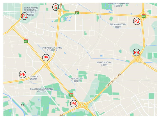
Figure 1.
Schematic diagram of the path with energy-aware ecological driving control.
If P3 is the destination, starting from S, and the maximum vehicle range is greater than or equal to path S with control vehicle traveling, it can be ensured that the vehicle will arrive at P3. If the vehicle travels from S to P2, the question will be how to make the shortest travel time to arrive, using the known starting point S and the distance between point S and point P2. Therefore, energy awareness and ecological driving control mainly solve the optimal control problem to ensure vehicles running between starting points and destinations when the battery power is known.
The main problems of energy sensing ecological driving control are as follows: realizing the maximum cruising distance is solved when the electric vehicle’s electric battery power is known. The other ecological driving control problem is the shortest travel time of the electric vehicle to the destination when given the distance and the onboard battery group’s quantity. The flow chart of solving the problem of real-time energy-sensing ecological driving control of the intelligent electric vehicle is shown in Figure 2.
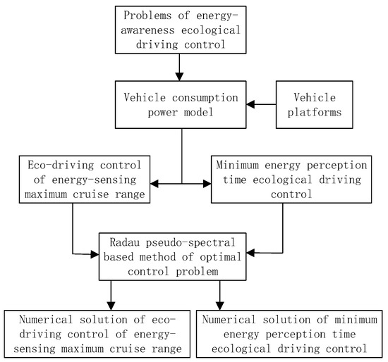
Figure 2.
The flow chart of solving the problem of real-time energy-sensing ecological driving control of the intelligent electric vehicle.
Based on Figure 2, the method is to establish the optimal control problem of economic driving. Firstly, the energy consumption model of the vehicle is established according to the vehicle platform, and then the maximum driving distance problem and the minimum energy consumption problem are established, respectively. Finally, the optimal control problem is solved based on the Radau pseudo-spectral method, and the numerical results are given.
3. Intelligent Electric Vehicle Platforms
3.1. Vehicle Platforms
The paper’s intelligent electric vehicle is modified from a Dongfeng electric sightseeing vehicle, as shown in Figure 3. The car’s original throttle, brake, and steering parts have been modified to achieve automatic driving. It is equipped with GPS/INS, four-wire laser radar, cameras, and other essential environmental perception equipment. We developed the vehicle’s low-level control module and designed a layered vehicle control computer system as the core of the planning and decision-making layer.
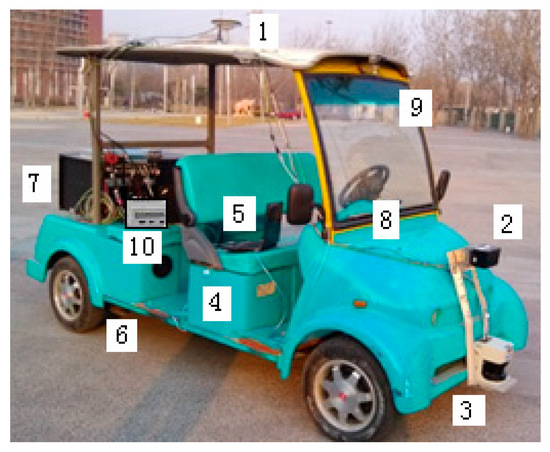
Figure 3.
Real car camera and configuration picture. (1) GPS/INS module. (2) IBEO LUX 2010. (3) LMS291. Four-battery group. (5) Planning decision computer. (6) Inverter and motor drive module. (7) Underlying control module. (8) Steering, throttle, and brake modules. (9) Camera. (10) DC energy meter.
In Figure 3, a DC electricity meter is used to measure the amount of battery energy consumed. In this way, the battery group’s remaining energy could be obtained, with the vehicle battery group’s total capacity minus the energy consumed.
3.2. Power System Structure and Working Principle
The vehicle uses a permanent magnet synchronous motor as the power drive unit, and the rear wheel drives the transmission system through a single gear drive. The DC battery bank provides power through a DC/AC inverter. In this way, the vehicle model is comprised of four parts: standard driveline, auxiliary load, DC/AC inverter, and motor, as shown in Figure 4.
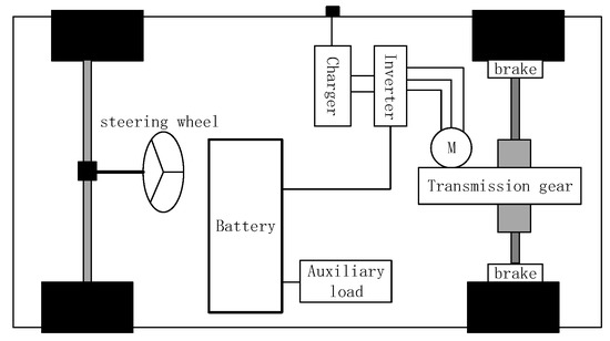
Figure 4.
Power system structure diagram.
4. Intelligent Electric Vehicle Platforms
4.1. Longitudinal Motion Model
The vehicle longitudinal motion model is the basic model, and the model covers the inertial vehicle dynamics and the efficiency of the powertrains used to predict the vehicle’s energy consumption [13]. For speed and acceleration of driving in electric vehicles, the force has the following relationship:
where is the force for the vehicle traction motor, is the acceleration resistance of the vehicle, is the vehicle’s wheels rolling resistance, is air resistance, is road slope resistance, and is vehicle quality. Additionally, is acceleration, is the rolling resistance constant, is the air resistance constant, is road slope, and is the acceleration of gravity. The parameter values are shown in Table 1.

Table 1.
Vehicle model parameters.
Representing the speed and distance as state variables, the vehicle longitudinal dynamics model for movement is:
4.2. Vehicle Consumption Power Model
An electric vehicle’s power consumption model reflects the relationship between vehicle energy consumption and vehicle motion index [18,19,20]. The vehicle power consumption model includes two parts: one part is used for the power consumption of the traction vehicle, and the other is used for the heat loss of the motor. It is:
where is the consumed power for the traction vehicle, and is the heat loss for motor power.
The driving speed of vehicles, shows as:
Assumptions is the motor current, the motor traction force is:
where is the motor’s armature constant, is the armature flux of the motor, is the gear reduction ratio, and is vehicle tire radius.
Assume that the motor armature winding resistance is , then the motor power for heat loss is:
Equations (4) and (5) are substituted into Equation (6). It will be as follows:
Thus, the total power consumption of the electric vehicle is:
In other words, Equation (8) shows the instantaneous output power for the car battery. In practice, when is negative, the value of Equation (8) may be negative. The reason is that the vehicle is in a state of brake energy regeneration at the time. Assuming that the vehicle travels on flat roads and road slope resistance is zero, Equation (8) does not consider road slope resistance.
Considering the influence of road slope resistance, the total power consumption of the electric vehicle is:
If the vehicle’s road slope can be measured, then the slope resistance can be obtained, the Equation (9) can be implemented online. In some papers, the road slope resistance is calculated as a vehicle distance function. It will make Equation (8) as the function of vehicle distance traveled, which increases the difficulty of processing Equation (9).
5. Intelligent Electric Vehicle Problems of Energy Sensing Ecological Driving Control
5.1. Eco-Driving Control of Energy-Sensing Maximum Cruise Range
Usually, the continuous range of electric vehicles on a single charge is lower than the fuel vehicle’s biggest distance. To ensure the electric vehicle arrives at the terminus or charging station, it needs to increase the electric vehicle’s longest continuous range. It can increase the electric vehicle’s maximum continuous range by extending the electric vehicle battery power capacity, but its weight and size limit this method. To this end, the known electric vehicle battery capacity, or the residual capacity of the current conditions, using other ways to solve the above problem, has become one area in the research content.
From Equation (1), it can be seen that overcoming various resistances during vehicle running becomes the main factor of power consumption. Moreover, Equation (8) or (9) reflect the relationship between electric vehicle power consumption and vehicle motion index. Vehicle acceleration and air resistance are closely related to vehicle motion indicators except for wheel rolling and road slope resistance.
According to Equation (8) or (9), the power consumed by electric vehicles can be changed by changing vehicle acceleration and speed. Therefore, based on the total power consumed by the electric vehicle in Equation (8) or (9), the electric vehicle’s maximum endurance distance can be increased by optimizing the vehicle acceleration under the condition of known residual power of the onboard battery. In this way, the ecological driving control problem of energy perception maximizing cruise distance is transformed into an optimal driving control problem.
Therefore, the eco-driving control of maximizing cruise distance with energy perception is expressed as:
s.t.
The equations shown in (10) are eco-driving performance indicators of electric energy maximum distance perception. Equation (11) is the vehicle longitudinal motion dynamics model. Furthermore, Equation (12) is the relationship between consumed electric energy and power. The combination of Equations (11) and (12) are state–space model constraint conditions, as performance indexes of Equation (10). Distance is , speed is , and vehicle power are state variables, and the vehicle acceleration is a control variable. Equations (13)~(15) are boundary constraints conditions.
is the maximum distance of running time, that was not specified in advance. is the maximum endurance distance to be solved. is the remaining vehicle battery power. Equations (13)~(15) show that the initial speed of the vehicle is 0, the starting distance of 0, the starting battery power as , and the terminus speed is 0, the destination distance is , and battery’s remaining power is (usually is not 0, here it can take 0).
Equation (10) also shows that when the vehicle battery remaining power as , the vehicle can run the maximum distance. Equation (16) is the battery power constraints condition, Equation (17) is the speed constraints condition, and Equation (18) is the vehicle acceleration constraints. These constraints conditions depend on physical vehicle parameters. Under the initial vehicle movement indicators, the remaining power consumption makes the vehicle’s distance the largest through optimal driving control when the vehicle arrives at the finish line motion index.
5.2. Minimum Energy Perception Time Ecological Driving Control
The main problem is the vehicle’s optimal driving control to reach the destination in the shortest driving time. Given the remaining electric quantity (initial electric quantity) and driving distance of the onboard battery pack, the vehicle can complete the known distance driving in the shortest time through the optimal driving control. That is the ecological driving control problem with the shortest energy perception time.
Minimum energy perception time ecological driving control shows:
s.t.
Equation (19) is the shortest ecological driving control performance index for energy awareness. is time to stay, as the performance index of Equation (19). The Equations (20) and (21) are similar to Equations (11) and (12). Equation (22) is the battery power constraints condition, and Equation (23) is the road boundary constraints known to vehicles running in advance. Equation (24) is for the speed boundary constraints, and the initial speed of 0 does not specify the end speed. Equation (25) is the battery power constraint. Equations (26) and (27) are the same as (17) and (18). In this way, Equations (22) and (23) shows that the initial energy is the battery group’s power in the vehicle, the distance is .
6. The Solution of Energy-Aware Ecological Driving Control
6.1. Solving Method of Optimal Control
Equations (10) and (19) are the typical optimal control problems with boundary constraints. There are many methods for solving these optimal control questions, such as the direct method, the indirect method [21], and the dynamic programming method (DPM) [22]. The indirect method is based on Pontriagin’s minimum principle to deduce the first-order necessary conditions of the optimal control. The optimal control is transformed into the Hamilton boundary value problem and then solved using numerical methods such as the shooting method. In recent years, the direct method has gradually become the mainstream method to solve optimal control, especially the pseudo-spectral method, which can obtain the optimal control problem’s numerical solution and provide accurate castrate variables. The pseudo-spectral method is used to solve the problem.
The problem is first transformed into a nonlinear programming problem (NLP) by pseudo-spectral discretization. It can be verified that the first-order necessary conditions of this nonlinear programming problem are equivalent to the conditions induced by the optimal control after pseudo-spectral dispersion. According to the pseudo-spectral method, the different standard pseudo-spectral method formats for selecting discrete grid points are Legendre–Gauss (LG), Legendre Gauss–Lobatto (LGL), Legendre–Gauss-Radau (LGR), and Chebyshev–Gauss–Lobatto (CGL), etc.
6.2. Radau Pseudo-Spectral Method (RPM)
The basic principle of RPM is as follows: the unknown state variables and control variables are discretized on a series of Legendre–Gauss–Radau (LGR) points, the global interpolation polynomial is constructed to approximate the state variables and control variables, and then the dynamic differential equation is replaced by the derivative of the state variables. In this way, a continuous system’s optimal control problem is transformed into an NLP problem subject to a series of algebraic constraints, which can be solved by the numerical method [22,23,24].
The Gauss pseudo-spectral optimization software (GPOPS) was used to solve the problem [25], and sequential quadratic programming (SQP) is for solving nonlinear programming. Take the maximum cruising distance perception of ecological energy control as an example, the state vector , vector control , take for Equation (10), for Equations (11) and (12), for (13) ~ (15).
6.3. Numerical Solution
Numerical solutions verify the validity and feasibility of the proposed method. Numerical simulation parameters are shown in Table 2.
Table 2.
Numerical simulation parameters.
6.4. Simulation Optimized Result of Energy-Aware Ecological Driving Control
Take the parameters listed in Table 1. One of the optimization problems of energy-sensing ecological driving control is shown in Figure 5. That shows the optimization results of vehicle driving distance, vehicle speed, acceleration, and battery quantity change. The initial battery capacity is 25,000 kJ. The driving distance of the vehicles is increasing continuously, with the maximum distance being 51.68 km. The traveling time is 4774 s. The battery is running low. In the beginning, the acceleration gradually decreased from the maximum (0.24512 m/s2).
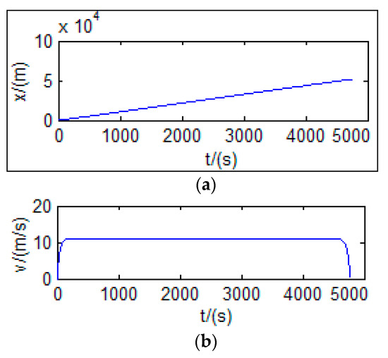
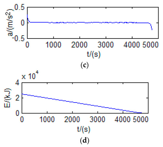
Figure 5.
Problem one optimization result: (a) the distance; (b) the speed; (c) the acceleration; (d) the power.
As can be seen from Figure 5a–d, the speed gradually increased (11.017 m/s). At about 113 s, the acceleration decreases to zero, and the velocity does not change anymore. At 4676 s, the acceleration starts to increase negatively (the maximum is −0.24525 m/s2), and the speed gradually decreases to 0. At this point, the vehicle has reached its maximum range, and the remaining battery capacity is also at a minimum.
According to Equation (8), the vehicle energy consumed is calculated. Compared with the results of Figure 5, the energy consumption without optimization is shown in Figure 6. In Figure 6, the vehicle’s driving distance is 51.68 km, which is the result of the previous optimization, and the vehicle’s energy consumption is more than the optimization result. ‘O’ in Figure 6 represents the optimization result when E is 25,000 kJ. Data of the maximum cruising distance of constant energy is shown in Table 3.
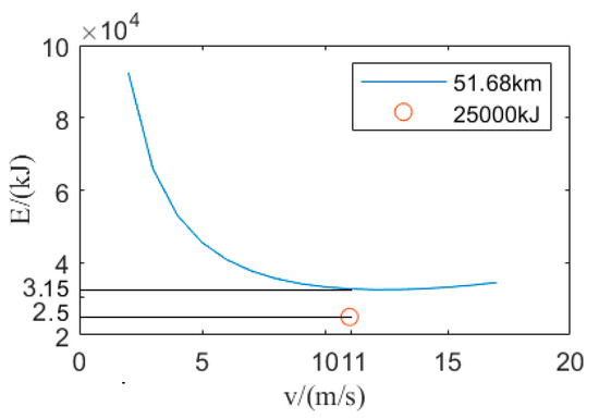
Figure 6.
Energy consumption compared with optimization and non-optimization.
Table 3.
Data of the maximum cruising distance of constant energy.
As shown in Figure 6, The energy consumptions of vehicles, traveling at the same distance, is compared. The results show that the optimization process has certain advantages. The energy consumption value obtained through optimization is less than 26% without optimization.
Without optimization, the vehicle driving distance calculated according to the battery power may not be in line with reality. Even if the driving distance is calculated, the battery’s remaining energy is insufficient to ensure the vehicle completes the driving distance.
Again, take the parameters listed in Table 2. The optimization results of the problem are shown in Figure 7. This chart shows that the optimization time conditions consist of battery energy, acceleration, velocity, and distance. Although the minimum travel time is obtained in Figure 7, the obtained optimization result cannot meet the speed constraints of the vehicle.
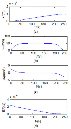
Figure 7.
Energy-aware ecological driving control optimization results: (a) the distance; (b) the speed; (c) the acceleration; (d) the power.
In Figure 7a–d, the initial battery power is 25,000 kJ, and the agreed driving distance is 10 km. Under the initial conditions, the shortest time to complete the distance is 232 s. The maximum acceleration is 4 m/s2, and the driving distance is completed at the maximum speed. Here, we remove the maximum speed constraint. The optimization results of the energy-sensing ecological driving control for other initial battery charges are shown in Table 4.
Table 4.
Minimum travel time data.
In Figure 7a–d, the speed trajectory optimization results can be seen, and that it cannot meet the Equation (26) constraints condition. According to Equation (18), the maximum acceleration is . Thus, the speed reaches the maximum value of time . After reaching maximum speed , the vehicle is running at the maximum speed uniformly. Similarly, the maximum time back from the vehicle is at a particular hour and can make the car’s speed from the maximum reduce to zero. In this way, the entire vehicle acceleration is divided into three sections as follows:
where , and are the unknown variables to be optimized and satisfy the constraints of the following conditions:
Equation (29) is the driving distance constraint condition, and Equation (30) is the power consumption constraint condition.
The initial conditions of the results shown in Figure 7 are taken, and the optimization results are obtained based on the conclusion of Equations (28)~(30) with the multiphase pseudo-spectral method, as shown in Figure 8. Each result in Figure 8 is divided into three periods corresponding to the three periods in Equation (28). The optimization speed result in Figure 8 satisfies the constraint condition of Equation (26). In Figure 7, the shortest time is about 232 s, while in Figure 8, the shortest time is 500 s. Although the shortest time in Figure 7 is less than that in Figure 8, with the condition that the driving distance has been 10.0 km meters, the known curves of driving distance, vehicle speed, vehicle acceleration, and energy consumption. The speed in Figure 6 does not meet the equation’s constraint condition (26). Therefore, under the constraint condition of Equation (26), the shortest time in Figure 8 is more practical.
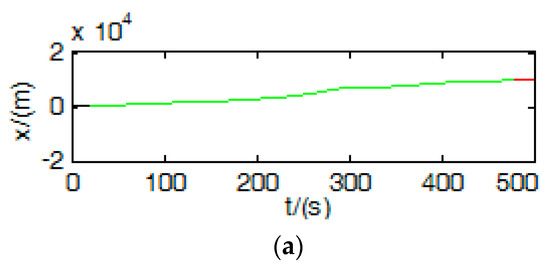
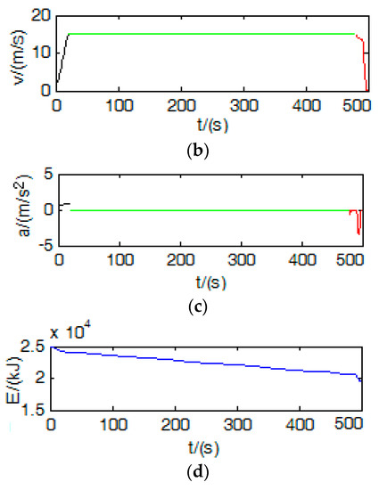
Figure 8.
Optimization results of the multiphase pseudo-spectral method for energy-aware ecological driving control: (a) the distance; (b) the speed; (c) the acceleration; (d) the power.
Compared with Figure 8, the vehicle travel time at different average speeds is shown in Figure 9. In Figure 9, the vehicle’s driving distance is 10 km, and the shorter the vehicle speed, the more travel time; The higher the vehicle speed, the less time will travel. In Figure 9, the vehicle travel time (625 s) is greater than 25% of the optimized travel time (500 s) in Figure 8. The results show that the vehicle travel time is the shortest after the optimization process when the vehicle travel distance is the same. ‘O’ in Figure 9 represents the optimization result when the driving distance is 10 km.
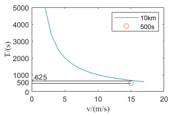
Figure 9.
Driving time compares with optimization and non-optimization.
7. Discussion
The two ECO problems of maximum travel distance and minimum energy consumption are studied, as shown in Figure 5 and Figure 6. It is shown that the obtained energy consumption value through optimization is less than that without optimization when the energy consumptions of vehicles, traveling at the same distance, is compared. In Figure 9, the results show that the vehicle travel time is the shortest after the optimization process when the vehicle travel distance is the same. The results also show that the optimization process has certain advantages. In the future, these results can be used as one of the strategies of vehicle battery management systems.
Through many simulation experiments, other critical data of optimization results in the initial battery quantity are shown in Table 3. The data in Table 3 are plotted as shown in Figure 10.
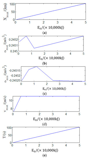
Figure 10.
Wiring diagram of energy consumption measurement. (a) The distance; (b) the max acceleration; (c) the min acceleration; (d) the speed; (e) the travel time.
As shown in Figure 10, the optimization results under the conditions of 50,000 kJ, 25,000 kJ, 12,000 kJ, 6000 kJ, and 600 kJ show that the method has wide application. Next, we will carry out the actual measurement. For the remaining power of the battery pack strategy in this paper, a DC energy meter will be used to measure the consumed DC energy. The remaining power of the battery pack can be obtained by subtracting the consumed power from the total power of the battery pack. The DC energy meter is installed at both ends of the battery pack of the experimental vehicle and can measure the voltage, output current, and DC energy at both ends of the battery pack. The electric energy meter has RS485 communication interface of the Modbus communication protocol. The DC electric energy measurement wiring diagram is shown in Figure 11.
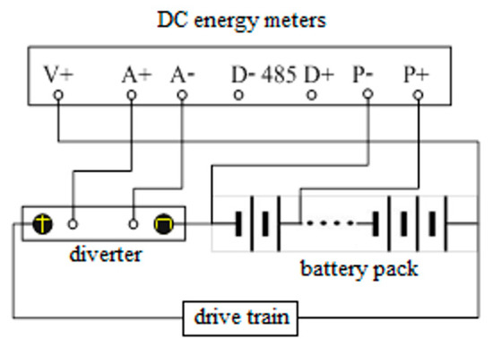
Figure 11.
Wiring diagram of energy consumption measurement.
8. Conclusions
The real-time energy-sensing ecological driving control problem of the pure electric vehicle is studied. In order to obtain the result of less energy for the same distance, the relationship between vehicle longitudinal motion dynamics and the electric vehicle energy consumption is analyzed, and the optimal control problem of maximum cruise distance and shortest cruise time is established. The optimized results of each performance index were obtained based on the Radau pseudo-spectral method. The shortest traveling time problem’s speed optimization results were based on the single-phase pseudo-spectral method and could not meet the speed constraint conditions. Under specific battery energy, the optimization problem of maximum driving distance is realized, and the energy of the battery consumed by the vehicle is the least. The residual energy of the vehicle battery pack is considered in the maximum driving distance problem. In addition, the residual energy of the battery pack is rarely considered in the maximum vehicle driving distance. In fact, according to Figure 6, if the residual energy of the vehicle battery pack is not considered, the result of the maximum driving distance is not realistic. Even if the driving distance is calculated, the battery’s remaining energy is not enough to ensure the vehicle completes the driving distance. The energy consumptions of vehicles, traveling at the same distance, are compared. The consumption obtained through optimization, is 26% less than the consumption of the vehicle that has not been optimized. Compared with the existing literature, for the application of intelligent vehicles, in the future, the acceleration trajectory in the optimization results can be used as the vehicle driving controller’s input, which can realize the vehicle is driving within its performance indicators. For the intelligent vehicle, the autonomous driving controller senses the remaining battery power in real-time and automatically realizes the intelligent vehicle’s ecological driving. Therefore, real-time energy-sensing ecological driving control has been added to the intelligent vehicle.
Author Contributions
H.H., D.L., X.L. and J.X. designed the analysis, developed the software, wrote the original and revised manuscript, and conducted data analysis and details of the work. H.H., X.L. and J.X. designed the research experiment, verified data, and conducted statistical analysis. H.H. and D.L. collected the data and conducted the analysis. J.X., X.L. and H.H. conceptualized and designed the research experiment, wrote the original/revised drafts, designed, re-designed, and verified image data analysis, and guided direction of the work. All authors have read and agreed to the published version of the manuscript.
Funding
This research was supported in part by the National Natural Science Foundation of China under Grants 61772576, 61975015, and 61379113, Henan Science and Technology Innovation Team under Grant CXTD2017091, Science and Technology Innovation Team of Colleges and Universities in Henan Province under Grant 18IRTSTHN013.
Data Availability Statement
No new data were created or analyzed in this study. Data sharing is not applicable to this article.
Acknowledgments
The authors would like to thank Bernard Jim and Joseph Spieles from Case Western Reserve University for their insightful comments, which have substantially improved the quality of this paper. We are also grateful to two anonymous reviewers for their constructive comments.
Conflicts of Interest
The authors declare no conflict of interest.
References
- Yang, D.; Jiang, K.; Zhao, D.; Yu, C.; Cao, Z.; Xie, S.; Xiao, Z.; Jiao, X.; Wang, S.; Zhang, K. Intelligent and connected vehicles: Current status and future perspectives. Sci. China Technol. Sci. 2018, 61, 1446–1471. [Google Scholar] [CrossRef]
- Neumann, I.; Franke, T.; Cocron, P.; Bühler, F.; Krems, J.F. Eco-driving strategies in battery electric vehicle use–how do drivers adapt over time? IET Intell. Transp. Syst. 2015, 9, 746–753. [Google Scholar] [CrossRef] [Green Version]
- Fredette, D.; Ozguner, U. Dynamic eco-driving’s fuel saving potential in traffic: Multi-vehicle simulation study comparing three representative methods. IEEE Trans. Intell. Transp. Syst. 2017, 19, 2871–2879. [Google Scholar] [CrossRef]
- Wang, J.; Rakha, H.A. Fuel consumption model for conventional diesel buses. Appl. Energy 2016, 170, 394–402. [Google Scholar] [CrossRef]
- Shankar, R.; Marco, J. Method for estimating the energy consumption of electric vehicles and plug-in hybrid electric vehicles under real-world driving conditions. IET Intell. Transp. Syst. 2013, 7, 138–150. [Google Scholar] [CrossRef]
- Barth, M.; Mandava, S.; Boriboonsomsin, K.; Xia, H. Dynamic ECO-driving for arterial corridors. In Proceedings of the 2011 IEEE Forum on Integrated and Sustainable Transportation Systems, Vienna, Austria, 29 June–1 July 2011; pp. 182–188. [Google Scholar]
- Li, S.E.; Xu, S.; Huang, X.; Cheng, B.; Peng, H. Eco-departure of connected vehicles with V2X communication at signalized intersections. IEEE Trans. Veh. Technol. 2015, 64, 5439–5449. [Google Scholar] [CrossRef]
- Schwickart, T.; Voos, H.; Hadji-Minaglou, J.-R.; Darouach, M.; Rosich, A. Design and simulation of a real-time implementable energy-efficient model-predictive cruise controller for electric vehicles. J. Frankl. Inst. 2015, 352, 603–625. [Google Scholar] [CrossRef]
- Wang, S.; Lin, X. Eco-driving control of connected and automated hybrid vehicles in mixed driving scenarios. Appl. Energy 2020, 271, 115233. [Google Scholar] [CrossRef]
- Dogan, D.; Boyraz, P. Smart traction control systems for electric vehicles using acoustic road-type estimation. IEEE Trans. Intell. Veh. 2019, 28, 486–496. [Google Scholar] [CrossRef]
- Guo, Q.; Angah, O.; Liu, Z.; Ban, X.J. Hybrid deep reinforcement learning based eco-driving for low-level connected and automated vehicles along signalized corridors. Transp. Res. Part C Emerg. Technol. 2021, 124, 102980. [Google Scholar] [CrossRef]
- Gan, L.; Topcu, U.; Low, S.H. Optimal decentralized protocol for electric vehicle charging. IEEE Trans. Power Syst. 2012, 28, 940–951. [Google Scholar] [CrossRef] [Green Version]
- Qin, H.; Zhang, W. Charging scheduling with minimal waiting in a network of electric vehicles and charging stations. In Proceedings of the Eighth ACM International Workshop on Vehicular Inter-Networking, New York, NY, USA, 23 September 2011; pp. 51–60. [Google Scholar]
- Sun, B.; Deng, W.; He, R.; Wu, J.; Li, Y. Personalized Eco-Driving for Intelligent Electric Vehicles; 0148-7191; SAE Technical Paper; SAE International: Kunshan, China, 7 August 2018. [Google Scholar]
- Dib, W.; Serrao, L.; Sciarretta, A. Optimal control to minimize trip time and energy consumption in electric vehicles. In Proceedings of the 2011 IEEE Vehicle Power and Propulsion Conference, Chicago, IL, USA, 5–8 September 2011; pp. 1–8. [Google Scholar]
- Petit, N.; Sciarretta, A. Optimal drive of electric vehicles using an inversion-based trajectory generation approach. IFAC Proc. Vol. 2011, 44, 14519–14526. [Google Scholar] [CrossRef]
- Wissam, D.; Chasse, A.; Sciarretta, A.; Moulin, P. Optimal energy management compliant with online requirements for an electric vehicle in eco-driving applications. IFAC Proc. Vol. 2012, 45, 334–340. [Google Scholar]
- Xie, Y.; Li, Y.; Zhao, Z.; Dong, H.; Wang, S.; Liu, J.; Guan, J.; Duan, X. Microsimulation of electric vehicle energy consumption and driving range. Appl. Energy 2020, 267, 115081. [Google Scholar] [CrossRef]
- Dib, W.; Chasse, A.; Moulin, P.; Sciarretta, A.; Corde, G. Optimal energy management for an electric vehicle in eco-driving applications. Control. Eng. Pract. 2014, 29, 299–307. [Google Scholar] [CrossRef]
- Wang, T.; Cassandras, C.G.; Pourazarm, S. Optimal motion control for energy-aware electric vehicles. Control. Eng. Pract. 2015, 38, 37–45. [Google Scholar] [CrossRef]
- Huntington, G.; Benson, D.; Rao, A. A comparison of accuracy and computational efficiency of three pseudospectral methods. In Proceedings of the AIAA Guidance, Navigation and Control Conference and Exhibit, Hilton Head, SC, USA, 20–23 August 2007; p. 6405. [Google Scholar]
- Ozatay, E.; Onori, S.; Wollaeger, J.; Ozguner, U.; Rizzoni, G.; Filev, D.; Michelini, J.; Di Cairano, S. Cloud-based velocity profile optimization for everyday driving: A dynamic-programming-based solution. IEEE Trans. Intell. Transp. Syst. 2014, 15, 2491–2505. [Google Scholar] [CrossRef]
- Zhang, W.; Zhao, Y.; Zhang, X.; Lin, F. Shared control for lane keeping assistance system based on multiple-phase handling inverse dynamics. Control. Eng. Pract. 2019, 93, 104182. [Google Scholar] [CrossRef]
- Wei, S.; Zou, Y.; Sun, F.; Christopher, O. A pseudospectral method for solving optimal control problem of a hybrid tracked vehicle. Appl. Energy 2017, 194, 588–595. [Google Scholar] [CrossRef]
- Wu, X.; He, X.; Yu, G.; Harmandayan, A.; Wang, Y. Energy-optimal speed control for electric vehicles on signalized arterials. IEEE Trans. Intell. Transp. Syst. 2015, 16, 2786–2796. [Google Scholar] [CrossRef]
Publisher’s Note: MDPI stays neutral with regard to jurisdictional claims in published maps and institutional affiliations. |
© 2021 by the authors. Licensee MDPI, Basel, Switzerland. This article is an open access article distributed under the terms and conditions of the Creative Commons Attribution (CC BY) license (https://creativecommons.org/licenses/by/4.0/).