Article

A Comparative Study on Power Flow Methods Applied to AC Distribution Networks with Single-Phase Representation

by
Oscar Danilo Montoya
1,2,*,
Alexander Molina-Cabrera
3 and
Jesus C. Hernández
4,*
1
Facultad de Ingeniería, Universidad Distrital Francisco José de Caldas, Bogotá 110231, Colombia
2
Laboratorio Inteligente de Energía, Universidad Tecnológica de Bolívar, Cartagena 131001, Colombia
3
Facultad de Ingeniería, Universidad Tecnológica de Pereira, Pereira 660003, Colombia
4
Department of Electrical Engineering, University of Jaén, Campus Lagunillas s/n, Edificio A3, 23071 Jaén, Spain
*
Authors to whom correspondence should be addressed.
Electronics 2021, 10(21), 2573; https://doi.org/10.3390/electronics10212573
Submission received: 19 September 2021 / Revised: 14 October 2021 / Accepted: 19 October 2021 / Published: 21 October 2021

Abstract

:
This paper presents a comparative analysis of six different iterative power flow methods applied to AC distribution networks, which have been recently reported in the scientific literature. These power flow methods are (i) successive approximations, (ii) matricial backward/forward method, (iii) triangular-based approach, (iv) product linearization method, (v) hyperbolic linearization method, and (vi) diagonal approximation method. The first three methods and the last one are formulated without recurring derivatives, and they can be directly formulated in the complex domain; the fourth and fifth methods are based on the linear approximation of the power balance equations that are also formulated in the complex domain. The numerical comparison involves three main aspects: the convergence rate, processing time, and the number of iterations calculated using the classical Newton–Raphson method as the reference case. Numerical results from two test feeders composed of 34 and 85 nodes demonstrate that the derivative-free methods have linear convergence, and the methods that use derivatives in their formulation have quadratic convergence.

1. Introduction

The estimation of the state variables in electrical systems corresponds to an essential study in electrical engineering [1], since the variables, i.e., the magnitudes and angles of the voltages in all the nodes of the network, allow us to determine the operative conditions of the grid [2], such as active and reactive power losses, grid efficiency, conductors’ chargeability, etc. The determination of these variables is widely-known in the literature as the power flow problem [3]. The mathematical representation and the solution of the power flow problem in power systems are typically developed using the Newton–Raphson method or its derived methods due to its efficiency and robustness regarding the number of iterations and the quadratic convergence rate [4]. In the case of electrical distribution grids, because of their configurations (radial or weakly meshed), power flow approaches that exploit the grid configuration to reduce the processing time required in the power solution are recommended [5]. For distribution systems, multiple power flow reformulations based on the graph structure of the grid can be found in the literature [6]. The most classical methods correspond to the backward/forward method and its derivations. Table 1 summarizes some references concerning power flow solutions in distribution grids in the last decades.
The power approaches listed in Table 1 can be classified in two main groups. The first group includes the power flow approaches that incorporate the distribution system graph by proposing recursive solutions without having recurring derivatives in their formulations [21,30], implying that these formulations only rearrange the power flow equations to obtain a recursive formula [23]. The second group of methodologies are based on Taylor’s series expansion of the power flow equations in real and complex domains that generate iterative solution methods based on linear approximations [24]. In the case of derivative-free methods, their convergence rate is typically linear, while the derivative-based methods have a quadratic convergence rate [31,32].
Based on the aforementioned revision of the state of the art regarding power flow methods applied to electrical AC distribution networks, in this research, we present a comparative study of the recently developed methodologies (from 2018 to 2021) that include four derivative methods and two derivative-based methods. To evaluate the effectiveness of these methods, the conventional Newton–Raphson method is considered the reference approach in two IEEE test feeders composed of 34 and 85 nodes, respectively, both with radial structure [33]. The numerical assessment considers the average processing time, the number of iterations, and the convergence rate analysis. The main contribution of this research is the summarization of the main recently developed power flow methods for AC distribution networks in a unique work, whereby researchers (also readers) can have multiple options to solve the power flow problem by selecting either derivative-free or derivative-based methods.
The main contributions of this research are as follows:
A complete comparison between recently developed power flow methods comprising four derivative-free and two derivative-based methods. These comparisons present convergence properties that are linear for derivative-free methods and quadratic for derivative-based approaches.
A new iterative method for power flow solution from the family of non-derivative approaches that present linear convergence and use the information of the nodal admittance matrix to obtain its recursive formula.
It is worth mentioning that, in the current literature, there exist some additional power flow approaches based on convex reformulations [34,35], such as semidefinite programming [36,37] and second-order cone programming [38,39]; however, these convex reformulations are typically solved with interior point methods since they are used in optimal power flow analyses, i.e., optimization problems wherein an objective performance (technical, economical, or environmental performance, or a combination of them) is considered. In this regard, these methods are outside the scope of this study since the main objective is to provide a comparison of the numerical methods for power flow solution.
This paper is structured as follows: Section 2 describes the general formulation of the power flow problem, and its subsections present each one of the studied methodologies, with all of them formulated in the complex domain. Section 3 mentions the main characteristics of the test feeders, which include two IEEE radial test feeders having 34 and 85 nodes and all the electrical information to implement the studied power flow methods. Section 4 presents the numerical validation of the studied methods using multiple consecutive evaluations that help determine the average processing time, number of iterations, and convergence rate properties. Section 5 discusses the main conclusions drawn from this research as well as possible future works.

2. Power Flow Formulations

This section presents the mathematical derivation of six power flow methodologies, which are applicable to single-phase distribution networks with radial structure. The methods under study are (i) successive approximations [23], (ii) matricial backward/forward method [21], (iii) triangular-based approach [22], (iv) product linearization method [24], (v) hyperbolic linearization method [28], and (vi) diagonal approximation approach. The main advantage of these power flow approaches is that they are formulated in the complex domain, thereby making their implementation simple in programming environments such as MATLAB or Python.

2.1. Formulation of the General Power Flow Problem

The power flow problem arises due to constant power loads in electrical power systems, which cause a hyperbolic relation between voltages and currents [19]. Let us define the net injected current in an arbitrary node as a function of the nodal admittance matrix and the voltage profile in all nodes of the network [1]:
I k = m N Y k m V m , k N I = Y bus V ,
where I k is the complex current injected at node k, Y k m is the complex component of the nodal admittance matrix that connects nodes k and m, V m is the complex value of the voltage at node m, I is the vector that contains all the nodal currents, Y bus is the square complex nodal admittance matrix, and V is the vector that contains all the nodal voltages. Note that N is the set that includes all the nodes of the network.
Now, if we refer to the definition of the average complex power, i.e., Tellegen’s theorem [40], we find the general definition of the power flow problem as follows:
S k = V k m = 1 n Y k m V m ,
where S k represents the conjugate of the net injected complex power at node k. Note that Equation (2) can be expressed in a compacted form as follows [19]:
S = diag ( V ) Y bus V .

2.2. Successive Approximation Power Flow Method

The successive approximation power flow method is a recursive power flow formulation of AC distribution networks initially proposed in [23], which deals with radial and meshed distribution networks. The main characteristic of this power flow method is its derivative-free formulation, which does not require the inverse of non-diagonal matrices at each iteration [6]. To express this power flow method, let us rearrange the power flow formula (3) as follows:
S s S d = diag V s 0 0 diag V d Y s s Y s d Y d s Y d d V s V d .
where S s and S d represent the complex conjugate injected power in the slack node and the complex conjugate demanded power in the load nodes, respectively; V s and V s are the complex conjugate voltages in the slack and demand nodes, respectively; Y s s , Y s d , Y d s , and Y d d are the sub-components of the admittance matrix that connect the slack and demand nodes among them.
Note that the first row in (4) is linear since the voltage in the slack node is perfectly known; this implies that if we know all the voltage values in the demand nodes, the power generation in the slack can be determined without performing any iterative process. In addition, note that the vector that contains all values of constant power consumption is preceded by a minus sign, which indicates that the demands in the nodes leave the distribution system.
From considering the second row of (4), one can observe a nonlinear relation among voltage demands, which implies that it is necessary to solve this formula using a numerical method. For doing so, let us obtain a recursive formula for solving V d from the second row of (4), which produces the following result.
V d = Y d d 1 Y d s V s + diag 1 V d S d .
To solve the recursive formula (5), it is necessary to add an iterative counter t to determine the final voltage value by starting from an initial point, which is typically assigned as the slack voltage, i.e., V d t = 1 V s , with 1 a vector constituting by ones with appropriate dimensions. For simplicity, we reassign the inverse of the admittance matrix Y d d 1 as Z d d , which is calculated once and stored for speeding up the iterative process, computationally speaking. The final recursive formula for the successive approximation method is the following.
V d t + 1 = Z d d Y d s V s + diag 1 V d t , S d .
The iterative process presented in (6) ends when the convergence criteria are met, which is selected as the difference of the voltage magnitudes between two consecutive iterations [23], i.e.,
max V d t + 1 V d t ε ,
which is tested at each iteration. Note that ε is the tolerance error, assigned as 1 × 10 10 [6].
Remark 1.
The convergence test for the successive approximation power flow method was provided in [23] using the Banach fixed-point theorem. This proves that the voltage profile always converges to the final solution independent of the starting point if and only if the operative point of the system is located far away from the voltage collapse point.

2.3. Matricial Backward/Forward Power Flow Method

The matricial backward/forward power flow method involves the generalization of the iterative sweep method for distribution grids using a nodal incidence matrix [21]. This reformulation method was initially proposed by the authors of [21,25]. To formulate this power flow method, let us define the branch-to-node incidence matrix as follows:
Branch-to-node incidence matrix: The matrix A R b × n is the branch-to-node incidence matrix that represents an electrical distribution network composed of b branches and n nodes if their currents are selected with arbitrary senses, and
A j k = 1 , if the current of the line j is leaving from the node k.
A j k = 1 , if the current of the line j is arriving at the node k.
A j k = 0 , if the line j is not connected to the node k.
With the incidence matrix, it is possible to link the voltages in all the branches, i.e., E b , with the voltage nodes by applying Kirchhoff’s Second Law to each branch, as follows:
E b = A s V s + A d V d ,
where A s is a column vector of the incidence matrix associated with the slack node, and A d is the remainder columns of the incidence matrix associated with the demand nodes.
Now, when Kirchhoff’s First Law is applied to each node of the network, assuming that all the demanded currents are leaving the system, i.e., they are negative, the following relation between the branch currents I b and the demanded currents is the following:
I s I d = A s A d I b .
An additional important relation between the branch voltages and currents are defined by Ohm’s law, i.e., I b = Y b b E b , where Y b b is the primitive admittance matrix that contains in its diagonal the inverse of the line impedance of each line. Using this relation in (8) and considering the second row of (9), the following formula is obtained.
I d = A d Y b b A s V s + A d V d .
In (10), it is possible to replace the nonlinear relation between demand voltages and powers, i.e., I d = diag 1 V d S d , and obtain a formula to solve V d as follows:
V d = A d Y b b A d 1 A d Y b b A s V s + diag 1 V d S d .
It is worth mentioning that if we redefine Y d d as A d Y b b A d and Y d s as A d Y b b A s , the recursive formula (10) associated with the matricial backward/forward is equivalent to the successive approximation power flow method as demonstrated by Briñez et al. in [6]. Finally, the iterative formula to solve the power flow problem using the matricial backward/forward approach takes the following form.
V d t + 1 = A d Y b b A d 1 A d Y b b A s V s + diag 1 V d t , S d .
Remark 2.
In the case of the matricial backward/forward power flow method as demonstrated in [21,41] and [25], its convergence independent of the starting voltage point through the application of the Banach-fixed point theorem.

2.4. Triangular-Based Power Flow Method

The triangular-based power flow method is a graph-based method incorporating an upper-triangular matrix that connects the demand and the branches’ currents. This method was initially proposed by [22]. To formulate the triangular-based power flow method, let us define the general structure of the upper-triangular matrix.
Upper-triangular matrix [42]: The matrix T R b × ( n 1 ) is an upper-triangular matrix that represents an electrical distribution network composed of b branches and n nodes, which has the following structure:
T j k = 1 , if the current of the line j support the current consumption at node k.
T j k = 0 , if the current of the line j does not support the current consumption at node k.
Now, if we apply Kirchhoff’s First Law at each node and rewrite the current consumption at each line as a function of the demanded currents, the following relation is obtained.
I b = T I d .
Note that in (13), Kirchhoff’s First Law was only applied to the demand nodes, and the slack nodes were not analyzed.
On the other hand, applying Kirchhoff’s Second Law to the closed-loop trajectory containing each demand node and the slack node yields the following results [27].
V d = 1 V s T E b .
In Equation (14), if we apply the Ohm’s law to each line voltage drop, i.e., E b = Z b b I b , and also it is considered (13) and the hyperbolic relation between voltages and powers, we get the following result.
V d = 1 V s T Z b b T diag 1 V d S d .
Once again, to determine the voltage profile at the demand nodes, we add an iterative counter t into the recursive formula (15), which produces the following iterative equation.
V d t + 1 = 1 V s T Z b b T diag 1 V d t , S d .
Remark 3.
To complete the iterative evaluation, the same detention criterion defined in (7) is applied. In addition, like the previously mentioned power flow methods, the triangular-based approach ensures convergence to the solution by applying the Banach fixed-point theorem [26].

2.5. Power Flow Approach Based on Voltage Product Linearization

The main characteristic of this power flow approach is that the Taylor series expansion is applied to obtain the equivalent linearized function that defines the product of two continuous variables around a desired operative point. This approach was recently proposed by Montoya et al. in [28]. This method linearizes the product among voltages in the second row of (5), i.e.,
diag V d Y d s V s + diag V d Y d d V d + S d = 0 ,
where the main interest of linearization is regarding the product diag V d Y d d V d , which can be represented mathematically as follows [28]:
diag V d Y d d V d = diag V d 0 , Y d d V d + diag V d Y d d V d 0 diag V d 0 , Y d d V d 0 ,
Now, if we substitute (18) in (17) and rearrange some terms, we get the following result:
diag V d Y d s V s + Y d d V d 0 + diag V d 0 , Y d d V d + S d diag V d 0 , Y d d V d 0 = 0 .
In Equation (19), it is possible to use the properties of diagonal matrices, which allows rewriting the product diag V d Y d s V s + Y d d V d 0 as diag Y d s V s + diag Y d d V d 0 V d ; this implies that Equation (19) takes the following form:
A V d + B V d = C ,
where
A = diag Y d s V s + diag Y d d V d 0 , B = diag V d 0 , Y d d , C = diag V d 0 , Y d d V d 0 S d .
Note that the solution of (20) requires to write it, into its real and imaginary components, i.e., V d = V d r + j V d i , A = A r + j A i , B = B r + j B i , and C = C r + j C i , which produce the following matricial relation:
A r + B r A i B i A i + B i B r A r V r V i = C r C i .
Note that the solution of Equation (21) is found by inverting the matrix that depends on the real and imaginary parts of the matrices B and B , which are also dependent on the linearizing point, i.e., V d 0 , in general, V d t , implying that the general solution of (21) takes the following form:
V r t + 1 V i t + 1 = A r t + B r t A i t B i t A i t + B i t B r t A r t 1 C r t C i t .
Remark 4.
The iterative process in (22) ends when the tolerance criterion is met as defined in Equation (7). In addition, note that the convergence criteria of the power flow method associated with the linearization of the voltage product has not yet been addressed in the scientific literature, which can be considered as a research opportunity in future works.

2.6. Power Flow Approach Based on Hyperbolic Voltage Relation Linearization

This power flow methodology is based on the linearization of the hyperbolic relation between voltages and powers in the power balance equation. This approach was initially proposed by Garces et. al in [19] and subsequently improved by Bocanegra et. al in [24]. This power formulation rewrites the power flow equation in the demand nodes, i.e., (17), as follows:
Y d s V s + Y d d V d + diag 1 V d S d = 0 ,
where the main idea is to linearize the third component of the left-hand side, i.e., diag 1 V d S d . This linearization is achieved through the application of Taylor series expansion, which produces, as presented in [24], the following result:
diag 1 V d S d = 2 diag 1 V d 0 , S d diag 2 V d 0 , diag V d S d .
Now, if we substitute (24) in (23) and use the properties of the diagonal matrices, the following result is reached.
diag 2 V d 0 , diag S d V d Y d d V d 2 diag 1 V d 0 , S d Y d s V s = 0 .
Note that the solution of (25) can be reached with the same representation of (20) if the matrices A and B and the vector C take the following structure:
A = diag 2 V d 0 , diag S d , B = Y d d , C = 2 diag 1 V d 0 , S d + Y d s V s .
Remark 5.
The iterative solution of (25) is reached with the recursive formula (22) using the aforementioned matrices A and B and the vector C . Its iterative search ends when the stopping criterion is met as defined in (7). Note that this method has not been reported in the literature regarding the convergence test, which offers another research opportunity to be addressed in future works.

2.7. Diagonal Approximation Power Flow Approach

A new iterative approach for solving power flow problem in electrical distribution networks is proposed in this section. This power flow formulation is a derivative-free approach that is created by rearranging Equation (17). Let us organize Equation (17) as follows:
V d = diag V d Y d d 1 S d + diag Y d s V s V d ,
Note that Equation (26) is recursive, which implies that it is necessary to add an iterative counter to solve it. The iterative formula for the diagonal approximation power flow approach takes the following form:
V d t + 1 = diag V d t , Y d d 1 S d + diag Y d s V s V d t , .
As observed in the previous cases, the detention criterion applicable to the recursive formula corresponds to the difference between both consecutive iterations. However, it is important to mention that the inverse of diag V d t , Y d d exists as Y d d is a dominant diagonal and diag V d t , is a diagonal whose component is always non-zero.
Remark 6.
The main characteristic of the diagonal approximation method is its similarity to the successive approximation power flow method (see Equation (6)) since both includes the inverse of the demand-to-demand admittance matrix; however, the diagonal approximation method considers the variations of voltage profiles in its numerical performance, which can affect the total processing time as well as the number of iterations.

3. Test Feeders

The assessment of each aforementioned power flow approach is carried out in two test feeders composed of 34 and 85 nodes, respectively. The main characteristics of the test feeders are mentioned below.

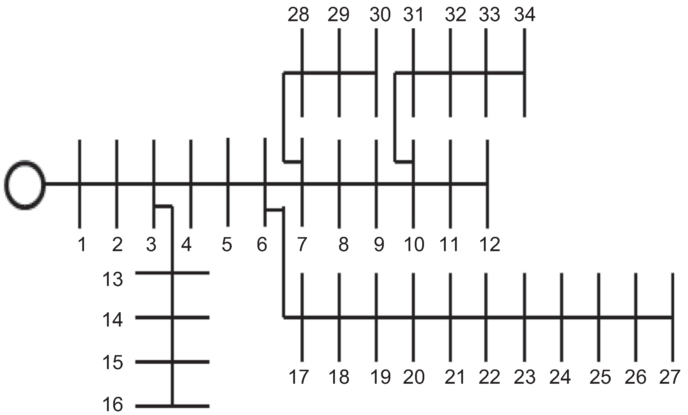
3.1. IEEE 34-Bus System

The IEEE 34-bus system is a radial distribution network comprising 34 nodes and 33 lines, which is operated at the substation bus in medium voltage levels with a nominal voltage rate of 11 kV. The electrical configuration of this test feeder is depicted in Figure 1. This test feeder has a total power consumption of 4636.50 + j 2873.50 kVA, which produces a total active and reactive power loss of 221.75 kW and 65.12 kvar, respectively.
The parametric information concerning this test system is reported in Table 2. Note that for all numerical simulations, we consider the voltage and power bases for this test system as 11 kV and 1000 kVA, respectively.

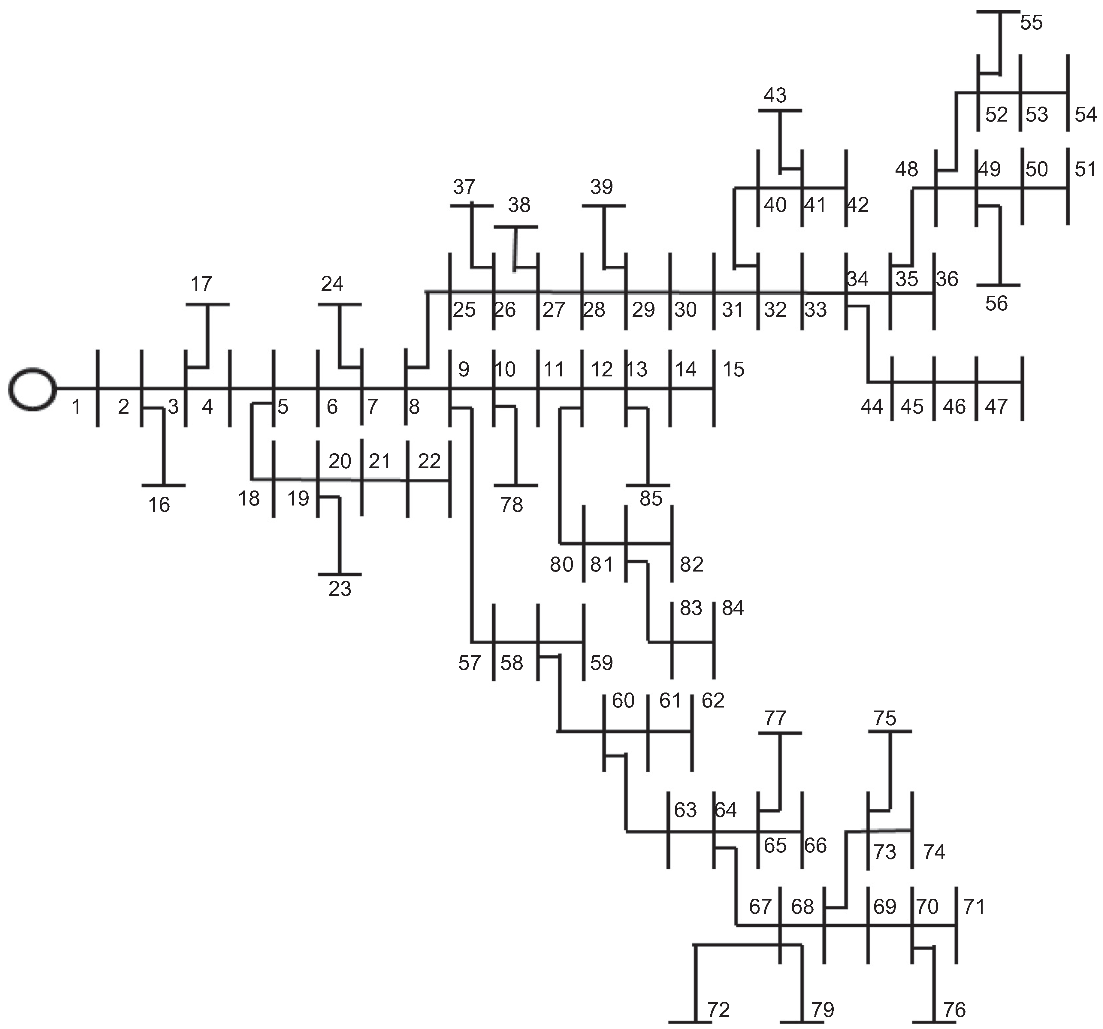
3.2. IEEE 85-Bus System

The IEEE 85-bus system has a radial medium-voltage distribution network composed of 85 nodes and 85 lines, operated with 11 kV. The total active and reactive power demand for this system is 2570.28 + j 2622.20 kVA. The electrical configuration of this system is provided in Figure 2, and all its parametric information has been taken from [43], which is given in Table 3.
For all numerical simulations, we consider the voltage and power bases for this test system as 11 kV and 1000 kVA, respectively. In reference, [33] reported the amount of active and reactive power losses for this test system: 316.12 kW and 198.60 kvar, respectively. These data are important since they form the losses reference for all the power flow methods studied.

4. Computational Implementation

To solve the power flow problem in the IEEE 34- and IEEE 85-bus systems, all the studied methods as well as the classical Newton–Raphson approach are considered [23]. All the numerical implementations are made in the MATLAB programming environment on a desk computer with INTEL(R) Core(TM) i5-3550, 3.50 GHz, and 8 GB RAM with 64-bit Windows 7 Professional.
To determine the average processing time of each power flow method as well as that of the Newton–Raphson approach, we evaluate each method 100,000 consecutive times. In addition, to determine the total power losses of the network, the following formula is used.
P loss = real V Y bus V .

4.1. Power Flow Results in the IEEE 34-Bus System

The power flow solution for the IEEE 34-bus system is provided in Table 4. Numerical results given in this table indicate that (i) all numerical methods lead to the same power losses value for the IEEE 34-bus system with the first six decimals being equal, i.e., 221.752357 kW; this confirms that all these methods are adequate to solve the power flow problem in radial distribution systems; (ii) the triangular-based power flow approach is the faster method to solve the power flow problem, taking about 0.1662 ms, which is followed by the successive approximation method with 0.1893 ms, while the slowest method is the classical Newton–Raphson method that takes almost 3 ms to solve the power flow problem; and (iii) the number of iterations of the derivative-free methods is higher than that of the methods using derivatives in their formulation; this is associated with the convergence rate, as will be discussed in the explanation of Figure 3.
Figure 3 presents the convergence rate of each power flow method studied and its comparison with the classical Newton–Raphson method. It is possible to observe from the figure that the derivative methods have a quadratic convergence, since the logarithm of the error log ( ϵ ) decreases with the square of the number of iterations, i.e., log ( ϵ ) = α t 2 , where α is a positive constant, while all the derivative-free methods converge linearly, i.e., log ( ϵ ) = α t , which implies that the number of iterations will be higher when compared with the derivative-based methods.
On the other hand, Figure 4 presents the percentages of the processing time of each studied power flow method when the Newton–Raphson is considered the reference method.
Three main results can be observed in this graphic: (i) even if the matricial backward/forward method and the successive approximation power flow method are mathematically equivalent, the former method takes additional processing time to solve the optimization problem, which is attributed to the need to construct an incidence matrix to generate the Y bus components; in contrast, the latter method constructs this matrix directly, avoiding additional matricial calculations that help reduce the time required to solve the power flow problem; (ii) the proposed diagonal approximation power flow method, even though similar to the successive approximation approach, takes about 4.6 times more time to solve the power flow problem, attributable to the fact that the diagonal method requires the calculation of the inverse matrix diag V d t , Y d d at each iteration, which extends the total processing time required to solve the problem; and (iii) the second slowest method is the product linearization method since it takes about 30.26 % of the time required in the Newton–Raphson method, followed by the diagonal approximation approach with 29.06 % ; however, numerical results concerning the IEEE 34-bus system show that all the methods improve the Newton–Raphson time by more than 69 % , which confirm their effectiveness in solving the studied problem.

4.2. Power Flow Results in the IEEE 85-Bus System

The power flow solution for the IEEE 85-bus system is given in Table 5, wherein the numerical results suggest that: (i) all methods calculate the total grid power losses with the same level of efficiency, i.e., up to six decimals, with the value being 316.117496 kW; (ii) the Newton–Raphson method takes more than 20 ms to solve the power flow problem, being the slowest method, while the triangular-based approach requires a total processing time of less than 0.6 ms, followed only by the successive approximation method with less than 1.1 ms; and (iii) the number of iterations for the Newton–Raphson method and the product linearization method increases to five iterations in comparison with the IEEE 34-bus system, while for the hyperbolic linearization approach, it remains at four iterations, and for the derivative-free methods number of iterations increase from 8 to 11 for this test feeder. These increments are mainly associated with the increment in the number of nodes of the system; however, in the case of the hyperbolic approximation, the rate of convergence is better, which demonstrates that it is possible to reach the desired convergence error with fewer iterations.
On the other hand, the results in Figure 5 confirm that the convergence rate of the derivative-based methods is quadratic, while that of the derivative-free approaches is linear, with the hyperbolic linearization approach showing the most efficient convergence rate with a slope higher than the Newton–Raphson method and the product linearization approach.
Finally, Figure 6 shows the comparison in percentage of the processing times of all the studied methods compared with the Newton–Raphson approach.
These processing times confirm that in the case of radial grids, the best power flow approach is the triangular-based power flow method, followed by the successive approximation method, with less than 2.7 % and 5.2 %, respectively, of the total processing time taken by the Newton–Raphson approach. In addition, all the methods, when compared with the Newton–Raphson approach, are possibly at least 74 % faster in the IEEE 85-bus system.

4.3. Additional Comments

Some important facts were generally observed with the power flow solutions for the IEEE 34- and IEEE 85-bus system when all the four derivative-free methods and the two derivative-based approaches are analyzed.
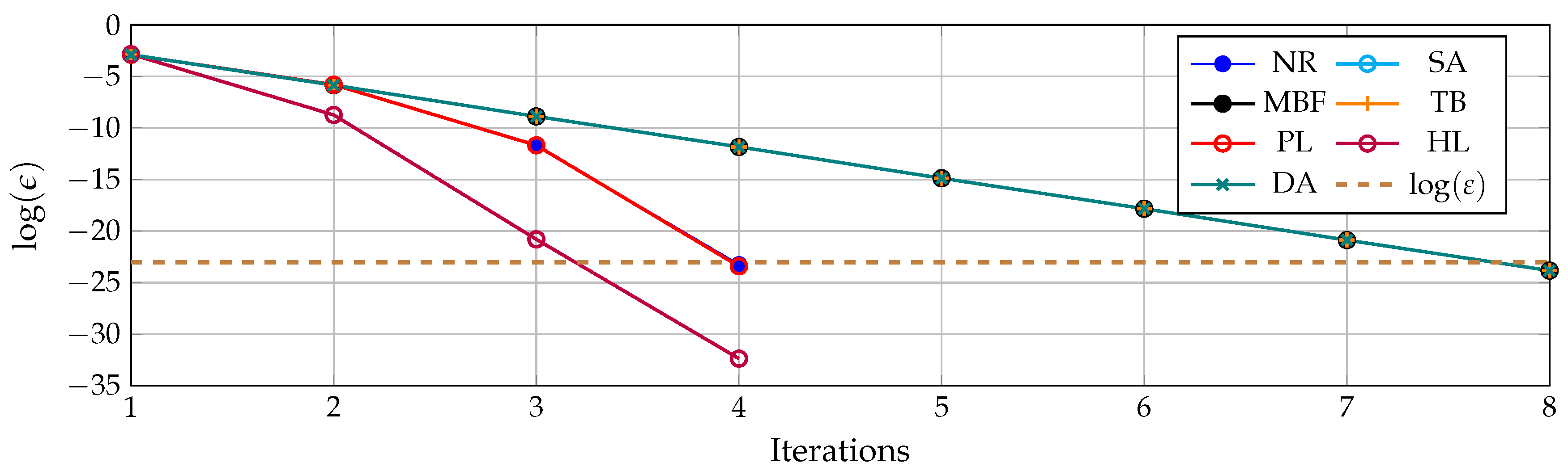
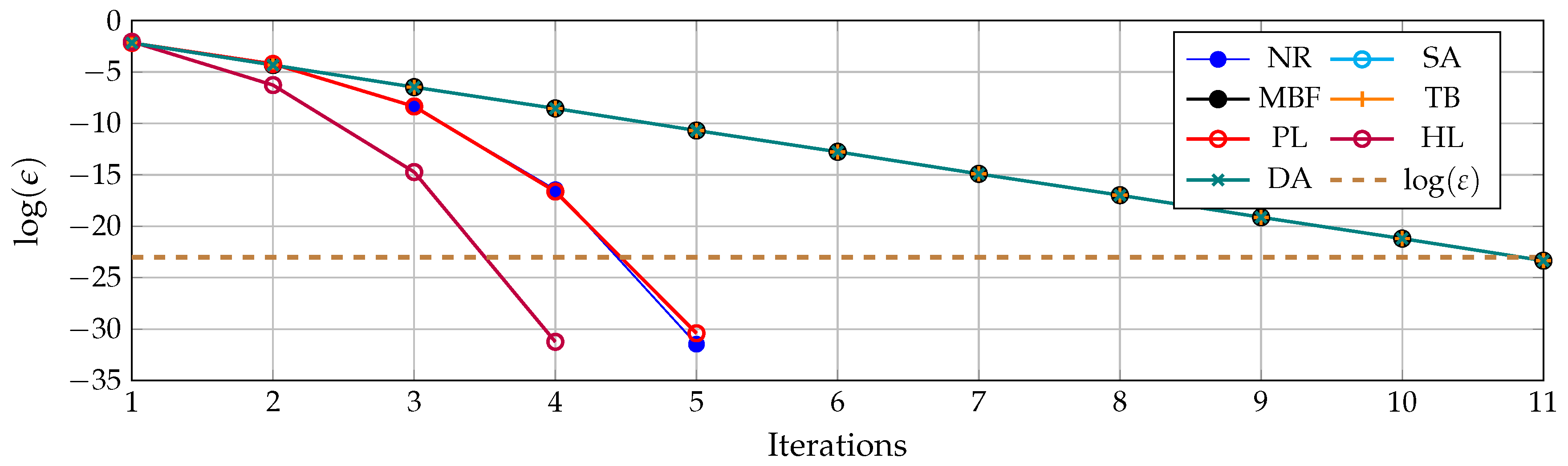
  • All derivative-free methods exhibit a linear convergence since their formulation is merely based on the reorganization of the power flow equations in an iterative manner, which implies that information regarding the gradient direction is not included to accelerate their performance regarding the number of iterations, while the derivative-based methods (including the Newton–Raphson approach) have in their formulation variable gains (marices) that help with the reduction of the voltage error after each iteration, which causes these methods to have a quadratic convergence rate.
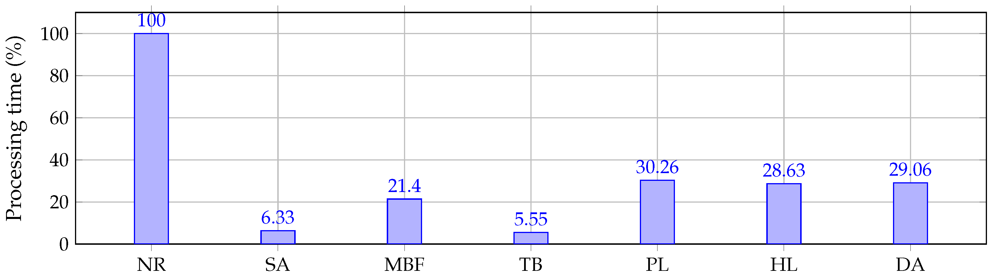
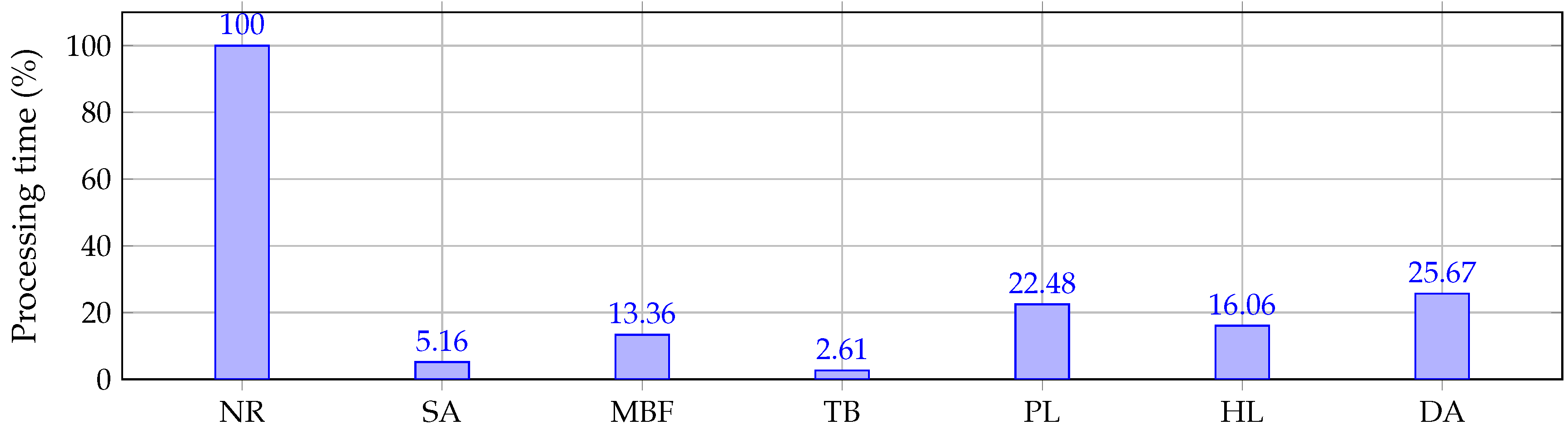
  • The diagonal approximation method, as well as the successive approximation method, is derived from the same power flow formula (see the second row of (4)); therefore, their numerical performance is very similar regarding the number of iterations and the convergence rate. However, the main advantage of the successive approximation method (6) over the diagonal approximation method (27) is the lesser total processing time required to solve the power flow problem since the former method uses a constant matrix that is once time inverted and stored, while the latter method requires inverse calculation at each time, leading to an additional computational effort.
  • All the studied methods provide the power flow solution regarding the final power losses estimation and voltage calculations; in fact, any one of them can be selected as a power flow tool for specialized optimization algorithms; however, the importance of knowing the total processing times deals with the selection of the most adequate method for specialized algorithms that evaluate thousands of power flows since, in these recursive optimization algorithms, small differences in the processing times of the power flow can produce important differences in the total execution time of the complete optimization algorithm.

5. Conclusions and Future Works

The classical problem of power flow calculation in AC distribution networks was addressed in this research with six different iterative methods that include four derivative-free and two derivative-based methods; the former methods exhibited linear convergence rate, while the latter methods present a quadratic convergence rate (including the Newton–Raphson approach). The convergence rate produced a direct effect on the total number of iterations to reach the desired tolerance error, with the hyperbolic linearization method with the highest slope that allows finding the solution of the power flow method in four iterations for the IEEE 85-bus system, while the remainder methods take five or more numbers of iterations to solve the power flow problem.
In terms of processing time, the triangular-based approach is the better methodology for radial distribution networks with processing times of 0.1662 ms and 0.5450 ms in the IEEE 34- and IEEE 85-bus systems, respectively, which is followed by the successive approximation method with 0.1893 ms and 1.0791 ms, respectively. However, all the derivative-methods starting with the present Newton–Raphson, product linearization, and hyperbolic linearization methods take higher processing times since, in each iteration, some matrices are updated to be inverted. The same happened with the diagonal approximation power flow method as was evidenced in both test feeders. Notwithstanding, for the IEEE 34- and IEEE 85-bus system, it was demonstrated that all the numerical methods improve the processing times of the Newton–Raphson approach more than 69 % and 74 % , respectively.
Future works could possibly deal with the following topics: (i) to extend the six studied methods to three-phase electrical networks with Δ and Y connected loads considering grid imbalances and also extend these methods for bipolar DC networks; and (ii) to compare the first iteration of these power flow methods (linear power flow solution) with different linear power approaches in the current literature to determine the best power flow approximation in AC distribution grids.

Author Contributions

Conceptualization, methodology, software, and writing—review and editing, O.D.M., A.M.-C. and J.C.H. All authors have read and agreed to the published version of the manuscript.

Funding

This research received no external funding.

Institutional Review Board Statement

Not applicable.

Informed Consent Statement

Not applicable.

Data Availability Statement

No new data were created or analyzed in this study. Data sharing is not applicable to this article.

Acknowledgments

This work was supported in part by the Centro de Investigación y Desarrollo Científico de la Universidad Distrital Francisco José de Caldas under grant 1643-12-2020 associated with the project: “Desarrollo de una metodología de optimización para la gestión óptima de recursos energéticos distribuidos en redes de distribución de energía eléctrica.” and in part by the Dirección de Investigaciones de la Universidad Tecnológica de Bolívar under grant PS2020002 associated with the project: “Ubicación óptima de bancos de capacitores de paso fijo en redes eléctricas de distribución para reducción de costos y pérdidas de energía: Aplicación de métodos exactos y metaheurísticos.”

Conflicts of Interest

The authors declare no conflict of interest.

References

  1. Murty, P. Load Flow Analysis. In Electrical Power Systems; Elsevier: Amsterdam, The Netherlands, 2017; pp. 527–587. [Google Scholar] [CrossRef]
  2. Albadi, M. Power Flow Analysis. In Computational Models in Engineering; IntechOpen: London, UK, 2020. [Google Scholar] [CrossRef] [Green Version]
  3. Tyagi, A.; Kumar, K.; Ansari, M.A.; Kumar, B. An efficient load flow solution for distribution system with addition of distributed generation using improved harmony search algorithms. J. Electr. Syst. Inf. Technol. 2020, 7, 1–16. [Google Scholar] [CrossRef] [Green Version]
  4. Milano, F. Analogy and Convergence of Levenberg’s and Lyapunov-Based Methods for Power Flow Analysis. IEEE Trans. Power Syst. 2016, 31, 1663–1664. [Google Scholar] [CrossRef]
  5. Acosta, C.; Hincapié, R.A.; Granada, M.; Escobar, A.H.; Gallego, R.A. An Efficient Three Phase Four Wire Radial Power Flow Including Neutral-Earth Effect. J. Control Autom. Electr. Syst. 2013, 24, 690–701. [Google Scholar] [CrossRef]
  6. Herrera-Briñez, M.C.; Montoya, O.D.; Alvarado-Barrios, L.; Chamorro, H.R. The Equivalence between Successive Approximations and Matricial Load Flow Formulations. Appl. Sci. 2021, 11, 2905. [Google Scholar] [CrossRef]
  7. Shirmohammadi, D.; Hong, H.; Semlyen, A.; Luo, G. A compensation-based power flow method for weakly meshed distribution and transmission networks. IEEE Trans. Power Syst. 1988, 3, 753–762. [Google Scholar] [CrossRef]
  8. Cheng, C.; Shirmohammadi, D. A three-phase power flow method for real-time distribution system analysis. IEEE Trans. Power Syst. 1995, 10, 671–679. [Google Scholar] [CrossRef]
  9. Haque, M. Efficient load flow method for distribution systems with radial or mesh configuration. IEE Proc. Gener. Transm. Distrib. 1996, 143, 33. [Google Scholar] [CrossRef]
  10. Teng, J.H. A modified Gauss–Seidel algorithm of three-phase power flow analysis in distribution networks. Int. J. Electr. Power Energy Syst. 2002, 24, 97–102. [Google Scholar] [CrossRef]
  11. Teng, J.H. A direct approach for distribution system load flow solutions. IEEE Trans. Power Deliv. 2003, 18, 882–887. [Google Scholar] [CrossRef]
  12. Yang, H.; Wen, F.; Wang, L. Newton-Raphson on Power Flow Algorithm and Broyden Method in the Distribution System. In Proceedings of the 2008 IEEE 2nd International Power and Energy Conference, Johor Bahru, Malaysia, 1–3 December 2008. [Google Scholar] [CrossRef]
  13. Lagace, P.J.; Vuong, M.H.; Kamwa, I. Improving Power Flow Convergence by Newton Raphson with a Levenberg-Marquardt Method. In Proceedings of the 2008 IEEE Power and Energy Society General Meeting—Conversion and Delivery of Electrical Energy in the 21st Century, Pittsburgh, PA, USA, 20–24 July 2008. [Google Scholar] [CrossRef]
  14. Augugliaro, A.; Dusonchet, L.; Favuzza, S.; Ippolito, M.; Sanseverino, E.R. A backward sweep method for power flow solution in distribution networks. Int. J. Electr. Power Energy Syst. 2010, 32, 271–280. [Google Scholar] [CrossRef]
  15. Lourenco, E.M.; Loddi, T.; Tortelli, O.L. Unified Load Flow Analysis for Emerging Distribution Systems. In Proceedings of the 2010 IEEE PES Innovative Smart Grid Technologies Conference Europe (ISGT Europe), Gothenburg, Sweden, 11–13 October 2010. [Google Scholar] [CrossRef]
  16. Jesus, P.D.O.D.; Alvarez, M.; Yusta, J. Distribution power flow method based on a real quasi-symmetric matrix. Electr. Power Syst. Res. 2013, 95, 148–159. [Google Scholar] [CrossRef]
  17. Tortelli, O.L.; Lourenco, E.M.; Garcia, A.V.; Pal, B.C. Fast Decoupled Power Flow to Emerging Distribution Systems via Complex pu Normalization. IEEE Trans. Power Syst. 2015, 30, 1351–1358. [Google Scholar] [CrossRef]
  18. Sianipar, G.H.M.; Setia, G.A.; Santosa, M.F. Implementation of Axis Rotation Fast Decoupled Load Flow on Distribution Systems. In Proceedings of the 2016 3rd Conference on Power Engineering and Renewable Energy (ICPERE), Yogyakarta, Indonesia, 29–30 November 2016. [Google Scholar] [CrossRef]
  19. Garces, A. A Linear Three-Phase Load Flow for Power Distribution Systems. IEEE Trans. Power Syst. 2016, 31, 827–828. [Google Scholar] [CrossRef]
  20. Bolognani, S.; Zampieri, S. On the Existence and Linear Approximation of the Power Flow Solution in Power Distribution Networks. IEEE Trans. Power Syst. 2016, 31, 163–172. [Google Scholar] [CrossRef] [Green Version]
  21. Shen, T.; Li, Y.; Xiang, J. A Graph-Based Power Flow Method for Balanced Distribution Systems. Energies 2018, 11, 511. [Google Scholar] [CrossRef] [Green Version]
  22. Marini, A.; Mortazavi, S.; Piegari, L.; Ghazizadeh, M.S. An efficient graph-based power flow algorithm for electrical distribution systems with a comprehensive modeling of distributed generations. Electr. Power Syst. Res. 2019, 170, 229–243. [Google Scholar] [CrossRef]
  23. Montoya, O.D.; Gil-González, W. On the numerical analysis based on successive approximations for power flow problems in AC distribution systems. Electr. Power Syst. Res. 2020, 187, 106454. [Google Scholar] [CrossRef]
  24. Bocanegra, S.Y.; Gil-Gonzalez, W.; Montoya, O.D. A New Iterative Power Flow Method for AC Distribution Grids with Radial and Mesh Topologies. In Proceedings of the 2020 IEEE International Autumn Meeting on Power, Electronics and Computing (ROPEC), Ixtapa, Mexico, 4–6 November 2020. [Google Scholar] [CrossRef]
  25. Montoya, O.D.; Gil-González, W.; Giral, D.A. On the Matricial Formulation of Iterative Sweep Power Flow for Radial and Meshed Distribution Networks with Guarantee of Convergence. Appl. Sci. 2020, 10, 5802. [Google Scholar] [CrossRef]
  26. Herrera-Briñez, M.C.; Montoya, O.D.; Molina-Cabrera, A.; Grisales-Noreña, L.F.; Giral-Ramirez, D.A. Convergence analysis of the triangular-based power flow method for AC distribution grids. Int. J. Electr. Comput. Eng. (IJECE) 2021, 12. [Google Scholar] [CrossRef]
  27. Montoya, O.D.; Giraldo, J.S.; Grisales-Noreña, L.F.; Chamorro, H.R.; Alvarado-Barrios, L. Accurate and Efficient Derivative-Free Three-Phase Power Flow Method for Unbalanced Distribution Networks. Computation 2021, 9, 61. [Google Scholar] [CrossRef]
  28. Montoya, O.D.; Rueda, L.E.; Gil-Gonzalez, W.; Molina-Cabrera, A.; Chamorro, H.R.; Soleimani, M. On the Power Flow Solution in AC Distribution Networks Using the Laurent’s Series Expansion. In Proceedings of the 2021 IEEE Texas Power and Energy Conference (TPEC), College Station, TX, USA, 2–5 February 2021. [Google Scholar] [CrossRef]
  29. Sereeter, B.; Markensteijn, A.; Kootte, M.; Vuik, C. A novel linearized power flow approach for transmission and distribution networks. J. Comput. Appl. Math. 2021, 394, 113572. [Google Scholar] [CrossRef]
  30. Kawambwa, S.; Mwifunyi, R.; Mnyanghwalo, D.; Hamisi, N.; Kalinga, E.; Mvungi, N. An improved backward/forward sweep power flow method based on network tree depth for radial distribution systems. J. Electr. Syst. Inf. Technol. 2021, 8, 1–18. [Google Scholar] [CrossRef]
  31. Deng, J.J.; Chiang, H.D. Convergence Region of Newton Iterative Power Flow Method: Numerical Studies. J. Appl. Math. 2013, 2013, 1–12. [Google Scholar] [CrossRef] [Green Version]
  32. Kulworawanichpong, T. Simplified Newton–Raphson power-flow solution method. Int. J. Electr. Power Energy Syst. 2010, 32, 551–558. [Google Scholar] [CrossRef]
  33. Prakash, D.; Lakshminarayana, C. Optimal siting of capacitors in radial distribution network using Whale Optimization Algorithm. Alex. Eng. J. 2017, 56, 499–509. [Google Scholar] [CrossRef] [Green Version]
  34. Molzahn, D.K.; Hiskens, I.A. Convex Relaxations of Optimal Power Flow Problems: An Illustrative Example. IEEE Trans. Circuits Syst. I Regul. Pap. 2016, 63, 650–660. [Google Scholar] [CrossRef] [Green Version]
  35. Garces, A. A quadratic approximation for the optimal power flow in power distribution systems. Electr. Power Syst. Res. 2016, 130, 222–229. [Google Scholar] [CrossRef] [Green Version]
  36. Bahrami, S.; Therrien, F.; Wong, V.W.; Jatskevich, J. Semidefinite Relaxation of Optimal Power Flow for AC–DC Grids. IEEE Trans. Power Syst. 2017, 32, 289–304. [Google Scholar] [CrossRef]
  37. Molzahn, D.K.; Holzer, J.T.; Lesieutre, B.C.; DeMarco, C.L. Implementation of a Large-Scale Optimal Power Flow Solver Based on Semidefinite Programming. IEEE Trans. Power Syst. 2013, 28, 3987–3998. [Google Scholar] [CrossRef]
  38. Yuan, Z.; Hesamzadeh, M.R. Second-order cone AC optimal power flow: Convex relaxations and feasible solutions. J. Mod. Power Syst. Clean Energy 2018, 7, 268–280. [Google Scholar] [CrossRef] [Green Version]
  39. Chowdhury, T.; Kamalasadan, S. A New Second-Order Cone Programming Model for Voltage Control of Power Distribution System with Inverter Based Distributed Generation. IEEE Trans. Ind. Appl. 2021, in press. [Google Scholar] [CrossRef]
  40. Ferreira, L. Tellegen’s theorem and power systems-new load flow equations, new solution methods. IEEE Trans. Circuits Syst. 1990, 37, 519–526. [Google Scholar] [CrossRef]
  41. Issicaba, D.; Coelho, J. Evaluation of the Forward-Backward Sweep Load Flow Method using the Contraction Mapping Principle. Int. J. Electr. Comput. Eng. (IJECE) 2016, 6, 3229. [Google Scholar] [CrossRef]
  42. Wang, X.F.; Song, Y.; Irving, M. Modern Power Systems Analysis; Springer: New York, NY, USA, 2008. [Google Scholar] [CrossRef]
  43. Zhang, D.; Fu, Z.; Zhang, L. An improved TS algorithm for loss-minimum reconfiguration in large-scale distribution systems. Electr. Power Syst. Res. 2007, 77, 685–694. [Google Scholar] [CrossRef]
Figure 1. Schematic interconnection among nodes in the IEEE 34-bus system.
Electronics 10 02573 g001
Figure 2. Schematic interconnection among nodes in the IEEE 85-bus system.
Electronics 10 02573 g002
Figure 3. Convergence performance of the studied methods in the IEEE 34-bus system.
Electronics 10 02573 g003
Figure 4. Processing time comparison for each studied power flow method when compared with the classical Newton–Raphson method in the IEEE 34-bus system.
Electronics 10 02573 g004
Figure 5. Convergence performance of the studied methods in the IEEE 85-bus system.
Electronics 10 02573 g005
Figure 6. Processing time comparison for each studied power flow method compared with the classical Newton–Raphson method in the IEEE 85-bus system.
Electronics 10 02573 g006
Table 1. Power flow methods for distribution networks.
Solution MethodologyYearTypeRefs.
Power flow solution using multi-port compensation technique for radial and meshed grids1988DF[7]
Backward/forward power flow method considering voltage-controlled nodes1995DF[8]
Current injection power flow method for radial and meshed distribution networks1996DF[9]
Improved Gauss–Seidel power flow method for distribution systems2002DF[10]
Direct power flow solution using LU matrix decomposition2003DF[11]
Improved Newton–Raphson method with Broyden’s method for distribution grids2008DB[12]
Improved Newton–Raphson method with Levenberg–Marquardt method for distribution grids2008DB[13]
Backward/forward power flow solution for radial and weakly meshed distribution grids2010DF[14]
Fast decoupled power flow method for emerging distribution grids2010DB[15]
Triangular formulation based on a real quasi-symmetry matrix2013DF[16]
Fast decoupled power flow method for distribution grids2015DB[17]
Axis rotation fast decoupled load flow on distribution systems2016DB[18]
Linear power flow approximation with hyperbolic linearization2016DB[19]
Linear power flow approximation based on the admittance matrix2016DB[20]
Graph-based power flow using an incidence matrix2018DF[21]
Graph-based power flow using an upper-triangular matrix2019DF[22]
Successive approximations power flow method that guarantees convergence2020DF[23]
Hyperbolic recursive linearization power flow method2020DB[24]
Matricial backward/forward power flow method that guarantees convergence and includes voltage-controlled nodes2020DF[25]
Triangular-based power flow method that guarantees convergence2021DF[26,27]
Product linearization power flow method2021DB[28]
Linearized power flow approach for transmission and distribution networks2021DB[29]
DB: Derivative-based; DF: Derivative-free.
Table 2. Parametric information regarding the IEEE 34-bus system.
km R km  ( Ω ) x km  ( Ω ) P k  (kW) Q k  (kW)km R km  ( Ω ) x km  ( Ω ) P k  (kW) Q k  (kW)
120.11700.0480230142.518190.20790.0473230142.5
230.10730.04400019200.18900.0430230142.5
340.16450.0457230142.520210.18900.0430230142.5
450.14950.0415230142.521220.26200.0450230142.5
560.14950.04150022230.26200.0450230142.5
670.31440.05400023240.31440.0540230142.5
780.20960.0360230142.524250.20960.0360230142.5
890.31440.0540230142.525260.13100.0225230142.5
9100.20960.03600026270.10480.018013785
10110.13100.0225230142.57280.15720.02707548
11120.10480.01801378428290.15720.02707548
3130.15720.0270724529300.15720.02707548
13140.20960.0360724510310.15720.02705734.5
14150.10480.0180724531320.20960.03605734.5
15160.05240.009013.57.532330.15720.02705734.5
6170.17940.0498230142.533340.10480.01805734.5
17180.16450.0457230142.5
Table 3. Parametric information regarding the IEEE 85-bus system.
km R km ( Ω ) x km ( Ω ) P k (kW) Q k (kW)km R km ( Ω ) x km ( Ω ) P k (kW) Q k (kW)
120.1080.0750034441.0020.41635.2835.99
230.1630.1120044450.9110.37835.2835.99
340.2170.1495657.1345460.9110.37835.2835.99
450.1080.0740046470.5460.2261414.28
560.4350.29835.2835.9935480.6370.26400
670.2720.1860048490.1820.07500
781.1970.82035.2835.9949500.3640.15136.2837.01
890.1080.0740050510.4550.1895657.13
9100.5980.4100048521.3660.56700
10110.5440.3735657.1352530.4550.18935.2835.99
11120.5440.3730053540.5460.2265657.13
12130.5980.4100052550.5460.2265657.13
13140.2720.18635.2835.9949560.5460.2261414.28
14150.3260.22335.2835.999570.2730.1135657.13
2160.7280.30235.2835.9957580.8190.34000
3170.4550.189112114.2658590.1820.0755657.13
5180.8200.3405657.1358600.5460.2265657.13
18190.6370.2645657.1360610.7280.3025657.13
19200.4550.18935.2835.9961621.0020.4155657.13
20210.8190.34035.2835.9960630.1820.0751414.28
21221.5480.64235.2835.9963640.7280.30200
19230.1820.0755657.1364650.1820.07500
7240.9100.37835.2835.9965660.1820.0755657.13
8250.4550.18935.2835.9964670.4550.18900
25260.3640.1515657.1367680.9100.37800
26270.5460.2260068691.0920.4535657.13
27280.2730.1135657.1369700.4550.18900
28290.5460.2260070710.5460.22635.2835.99
29300.5460.22635.2835.9967720.1820.0755657.13
30310.2730.11335.2835.9968731.1840.49100
31320.1820.0750073740.2730.1135657.13
32330.1820.0751414.2873751.0020.41635.2835.99
33340.8190.3400070760.5460.2265657.13
34350.6370.2640065770.0910.0371414.28
35360.1820.07535.2835.9910780.6370.2645657.13
26370.3640.1515657.1367790.5460.22635.2835.99
27381.0020.4165657.1312800.7280.3025657.13
29390.5460.2265657.1380810.3640.15100
32400.4550.18935.2835.9981820.0910.0375657.13
40411.0020.4160081831.0920.45335.2835.99
41420.2730.11335.2835.9983841.0020.4161414.28
41430.4550.18935.2835.9913850.8190.34035.2835.99
Table 4. Power flow performance in the IEEE 34-bus system.
MethodPower Losses (kW)No. of IterationsProc. Time (ms)
Newton–Raphson (NR) 42.9929
Successive approximations (SA) 80.1893
Matricial backward/forward (MBF) 80.6405
Triangular-based (TB)221.75235780.1662
Product linearization (PL) 40.9057
Hyperbolic linearization (HL) 40.8568
Diagonal approximation (DA) 80.8696
Table 5. Power flow performance in the IEEE 85-bus system.
MethodPower Losses (kW)No. of IterationsProc. Time (ms)
Newton-Raphson (NR) 520.8949
Successive approximations (SA) 111.0791
Matricial backward/forward (MBF) 112.7924
Triangular-based (TB)316.117496110.5450
Product linearization (PL) 54.6976
Hyperbolic linearization (HL) 43.3564
Diagonal approximation (DA) 115.3632
Publisher’s Note: MDPI stays neutral with regard to jurisdictional claims in published maps and institutional affiliations.

