SPSO Based Optimal Integration of DGs in Local Distribution Systems under Extreme Load Growth for Smart Cities

Abstract

Renewable energy-based distributed generators (DGs) are gaining more penetration in modern grids to meet the growing demand for electrical energy. The anticipated techno-economic benefits of these eco-friendly resources require their judicious and properly sized allocation in distribution networks (DNs). The preeminent objective of this research is to determine the sizing and optimal placing of DGs in the condensed DN of a smart city. The placing and sizing problem is modeled as an optimization problem to reduce the distribution loss without violating the technical constraints. The formulated model is solved for a radial distribution system with a non-uniformly distributed load utilizing the selective particle swarm optimization (SPSO) algorithm. The intended technique decreases the power loss and perfects the voltage profile at the system’s nodes. MATLAB is used for the simulation, and the obtained results are also validated by the Electrical Transient Analysis Program (ETAP). Results show that placing optimally sized DGs at optimal system nodes offers a considerable decline in power loss with an improved voltage profile at the network’s nodes. Distribution system operators can utilize the proposed technique to realize the reliable operation of overloaded urban networks.

1. Introduction

Electrical power demand is exponentially growing due to more urbanization, commercialization and industrial development. This exponential growth in demand poses operational challenges in power utilities [1,2,3]. The current infrastructure is insufficient to support such immense power demand. The congestion in transmission lines may lead to instability in the power system [4,5]. The main goal of power system operation is to encounter the request at all locations within the existing power network, both as economically and reliably as possible. However, the surge in power demands has originated several threats to the operation of distribution networks (DNs) [6]. It is a big challenge for the existing power system to handle extra demand requirements due to excessive population growth and smart cities projects for rural areas extensions.

Electricity generation in the traditional power grid is generally from fossil, hydro, nuclear resources, etc. Inherent needs of the conventional plants require their construction at remote areas far-off from the load center [7]. An adequate transmission network (may be hundreds of kilometers long) is then required to supply this generated energy to the load side. Since the existing lines are congested, and the installation of new lines requires huge investment. Therefore, researchers are looking for ways to defer this investment without compromising the stable grid operation. Moreover, lengthy lines originate more power losses and voltage drops. The high voltage drops, and power losses result in overheating and damaging of equipment [8]. It has been explored that transmission and distribution losses have a significant contribution to total power system losses. However, distribution losses are less than transmission line losses in power systems [9].

The development of technologies related to the internet of things (IoT), artificial intelligence (AI), blockchain and big data encourages power system operators to modernize power grid and smart city development [10,11,12]. It is always significant to have an efficient power system as greater losses distress the overall economy [13,14,15]. An efficient power system that meets demand uncertainties is helpful to generate deferent flexible options to initiate demand response (DR) actions [16,17]. To handle uncertainties in demand, modifications in the existing power system are required. Due to the effective amendment in the power system, private firms will be interested in investing in the supply system to encounter the active power request at each node and make it profitable for the whole community [18]. One better way of decreasing the losses is to incorporate the distributed generators (DGs) at appropriate locations in the distribution system [19]. Optimal DGs allocations are helpful in achieving improved voltage profile, reduced power losses and defer investments in transmission infrastructure [20,21]. DGs may be traditional or non-traditional and are usually connected in DNs near load centers [22]. Based on power injection, these are classified into four categories [23]:

(a)

Injects only real power to the system. Examples are solar photovoltaic and fuel cells.

(b)

Injects only reactive power to the system. Examples are synchronous condensers.

(c)

Injects both real and reactive powers (P and Q) into the system. Examples are synchronous generators, i.e., steam turbines and cogeneration.

(d)

Injects real power but absorbs reactive power. Examples are synchronous condensers.

DGs, especially based on renewable energy resources (RERs), are more emerging than centralized power generation. When appropriately installed, DGs decline power loss considering power stability, voltage profile and environmental conditions [24,25]. So, optimal placement of DG is crucial; otherwise, it can further increase the power loss and originate more pronounced voltage fluctuations. This paper proposes a new selective particle swarm optimization (SPSO) approach to find optimal DGs size and location. This approach aims to catch all bus voltages within acceptable limits with minimum deviation and minimum total power loss in the system based on economic and operational objectives from the DGs and grid side. The effectiveness of the proposed method is validated using data of a real 11 kV feeder with a non-uniform load growth characteristic, which is a part of the Gujranwala electric power company (GEPCO), Pakistan. The feeder is also simulated on ETAP using optimal DGs sizes and locations obtained by SPSO, and results validate the effectiveness of the proposed method.

The rest of the paper’s organization is as follows: Section 2 presents the review of research work related to the DGs sizing and siting problem. Section 3 describes the mathematical formulation of the problem and explains the proposed methodology for its solution using SPSO. Section 4 presents the distribution network used for the case study, and various SPSO simulation parameters of SPSO are presented. Section 5 contains simulation results for different cases with relevant discussion. The last Section 6 concludes the paper.

2. Related Work

Researchers have analyzed the problem of precise and accurate optimal placement of DG in the DNs to realize reduced losses and stable voltages utilizing different approaches. Various artificial intelligence and hybrid techniques have been proposed in the literature in addition to traditional approaches.

In References [10,21,22,23,24,25], the authors implemented several approaches for optimal DGs location. In References [26,27], an analytical method based on generalized reduced gradient was used to an analytical method based on generalized reduced gradient was used to locate DGs optimally in a meshed network for maximum benefits. Authors in [28,29] determined the level of penetration of photovoltaic (PV) units in a distribution network using the linear programming (LP) optimization technique. Various DG assessment measures such as improvement of voltage profile, line-losses and environmental aspects using multi-objective functions applicable to single or multiple DGs had been investigated in [30]. Using metaheuristics or AI, researchers have strived to find practical solutions in the best possible way for energy management and integration of DGs [31,32,33]. Genetic Algorithm (GA) is the popular metaheuristic approach developed by Holland. Its search procedure is based on natural selection and genetics principles. The theory of natural evolution inspires it, and its various steps include selection, crossover, mutation and inheritance. In Reference [34], the optimal allocation of DG under load and generation uncertainties was studied through evolutionary approaches. The 33-node IEEE test network was used for the evaluation. The authors achieved excellent results of voltage stability and loss reduction using GA in [31], improved extended GA, a combination of GA and analytical methods in [35,36], respectively.

In literature, Particle Swarm Optimization (PSO) has been extensively used for optimal DG locating and sizing [37]. Eberhart and Kennedy developed this valuable technique in 1995 and found it useful in optimizing multidirectional functions [23]. Authors in [3,38,39,40] implemented PSO to achieve the economic dispatch of multiple units. Due to parallel search capability, PSO can approach faster in accomplishing a global solution. Several research works have used PSO in combination with other techniques to gain more precise and accurate results. Hybrid GA-PSO [41], PSO and Linearized AC load flow [39], PSO-Compromise Programming [42], fuzzy approach and PSO [43] and discrete PSO-OPF [44] are some of the hybrid approaches. More comprehensive reviews on the DGs optimization problem can be observed in [45,46], where different algorithms and methods have been discussed.

From the literature review, it is evident that the optimized DG allocation and sizing problem remained the focus of researchers for multiple benefits at an economical cost. Traditional analytical approaches are nearly obsolete, and the modern trend is to use various variants of meta-heuristic techniques due to their simplicity, less computational effort and fast convergence. Therefore, a metaheuristic SPSO technique is proposed in this work to solve the DG placement and sizing problem.

3. Problem Formulation and Proposed Solution

This study’s primary objective is to reduce total DN power loss and the deviation of voltage from nominal voltage while meeting the equality and inequality constraints. The DG allocation and sizing problem is modeled as a multivariate optimization problem to realize the efficient operation of DN without compromising its voltage stability. Description of the proposed mathematical model and solution technique is presented in this section.

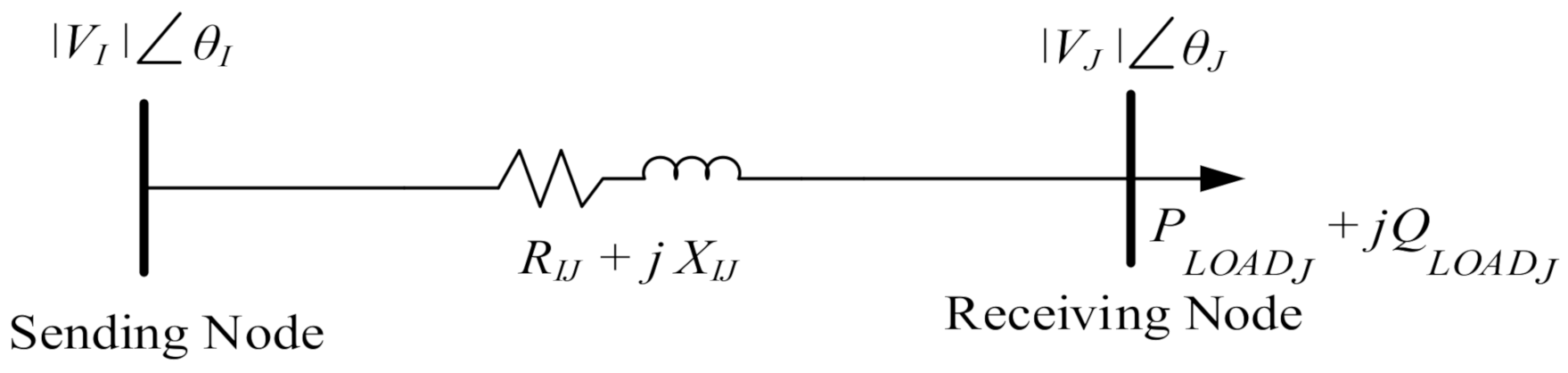
3.1. Mathematical Model

Let’s assume that N is the total number of buses, $P_I$ and $Q_I$ are the real and reactive power flows from bus $I$ to bus $I+1$, where bus voltage at the bus $I$ is $V_I$ and resistance of the line connecting the bus $I$and $I+1$ is depicted as $R_{I+1}$. Now the objective function is given by (1) where $f_1$ and $f_2$ represent the objectives related to real power loss $P_{L }$and voltage deviation ($V_{ID}$), respectively.

$$\mathrm{Minimize} Objective Function=W_1\times f_1+W_2\times f_2$$

(1)

$$f_1= P_{L }={\displaystyle \sum }_{I=1}^B{P}_{L_I}$$

(2)

$$f_2=V_{ID }={\displaystyle \sum }_{I=1}^N{(V_I-V_{REF})}^2$$

(3)

Here $W_1$ and $W_2$ are weighting factors acting as priority setters for enhancement of voltage stability and decrease of power loss, respectively. $B$represents the total system’s branches.

$$P_{L_I}=\frac{P_I{}^2+Q_I{}^2}{V_I{}^2}\times R_{I+1}$$

(4)

$$voltage deviation at node I = V_I-V_{REF}$$

(5)

$$W_1+W_2=1$$

(6)

3.1.1. Inequality Constraints

The supply voltages of the system must be within the permissible limits to avoid derating of the equipment.

$$V_I^{min} \le │V_I│\le V_I^{max}$$

(7)

So, the minimum and maximum voltages are 0.95 $V_{REF}$ and 1.05 $V_{REF}$, respectively, as per IEEE international standards [47] for the voltage drop in the DN for the proper safe operation of sensitive electrical equipment.

DG output is also constrained to remain within the permissible limits of reactive power (Q_DG), apparent power (S_DG), active power (P_DG) and voltages ($V$_DG) as represented in (8)–(11).

$${\mathrm{S}}_{DG}^{min} \le S_{\mathrm{DG}}\le S_{DG}^{max}$$

(8)

$${\mathrm{P}}_{DG}^{min} \le P_{\mathrm{DG}}\le P_{DG}^{max}$$

(9)

$$Q_{DG}^{min} \le Q_{\mathrm{DG}}\le Q_{DG}^{max}$$

(10)

$$V_{DG}^{min} \le V_{DG} \le V_{DG}^{max}$$

(11)

So, the size of DG is also pre-selected between 10–60% of the total system demand. The power factor ($P.F{.}_{DG}$) is the preceding but not the least essential quantity, which is previously established to operate at a practical value, which is 0.85.

$$P.F{.}^{min} \le P.F{.}_{DG} \le P.F{.}^{max}$$

(12)

3.1.2. Equality Constraints

These constraints are used to ensure power balance. For secure operation, the total power produced in a system must be equal to the amount of power demanded by the load plus the losses throughout the power system network. These constraints are reproduced in (13) and (14).

$$P_{Grid}+{\displaystyle \sum }_{J=1}^K{P}_{D{G}_J}-{\displaystyle \sum }_{I=1}^N{P}_{Loa{d}_I}-P_L=0$$

(13)

$$Q_{Grid}+{\displaystyle \sum }_{J=1}^K{Q}_{D{G}_J}-{\displaystyle \sum }_{I=1}^N{Q}_{Loa{d}_I}-Q_L=0$$

(14)

Here $P_{D{G}_J}$ and $Q_{D{G}_J}$ are real and reactive power of DG $J$. $K$ is the total number of DGs that are two in our cases. $P_{Loa{d}_I}$ and $Q_{Loa{d}_I}$ are the real and reactive power loads at bus $I$, respectively, whereas $P_L$ and $Q_L$ are the net active and reactive powers loss, respectively. $P_{Grid}$ and $Q_{Grid}$ denote the values of active and reactive powers drawn from the grid.

The total $P$ and $Q$ injected in the bus $I$ are given in (15) and (16).

$$P_I=\left|V_I\right|{\displaystyle \sum }_{J=1}^N\left|V_J\right| \left[g_{IJ}\cos \left({\theta }_I-{\theta }_J \right)+b_{IJ}\sin \left({\theta }_I-{\theta }_J \right)\right]$$

(15)

$$Q_I=\left|V_I\right|{\displaystyle \sum }_{J=1}^N\left|V_J\right| \left[g_{IJ}\sin \left({\theta }_I-{\theta }_J \right)+b_{IJ}\cos \left({\theta }_I-{\theta }_J \right)\right]$$

(16)

Here $V_I$ and $V_J$are the voltage magnitudes of bus$I$ and $J$, whereas θ_I and θ_J are the voltage angles of bus $I$ and $J$, respectively, as depicted in Figure 1. $g_{IJ}$ and $b_{IJ}$ are the real and imaginary parts of admittance between bus$I$ and $J$. The values of $P$, $Q$ and $V$ in the main function are computed by the utilization of power flow algorithm for radial distribution networks that conduct forward and backward sweeps to calculate the branch current and node voltages in the distribution system.

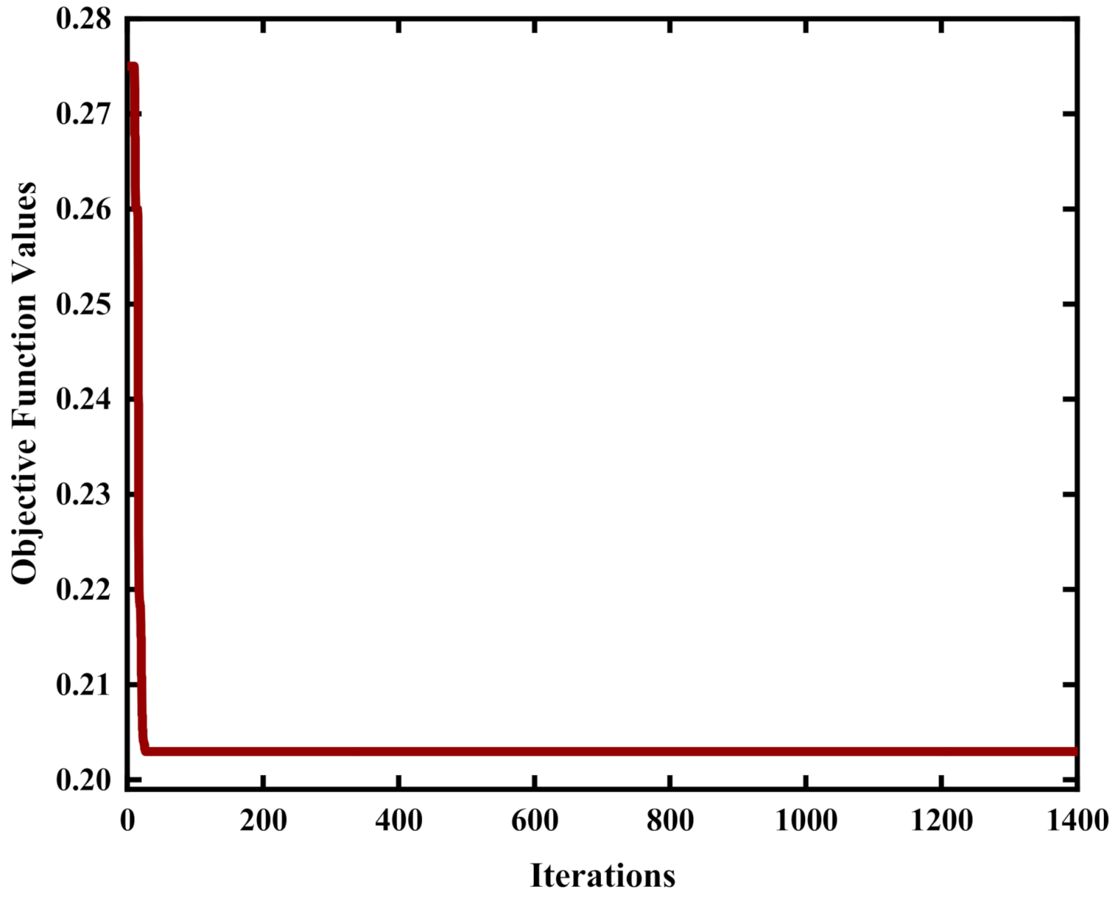
3.2. Proposed SPSO Algorithm

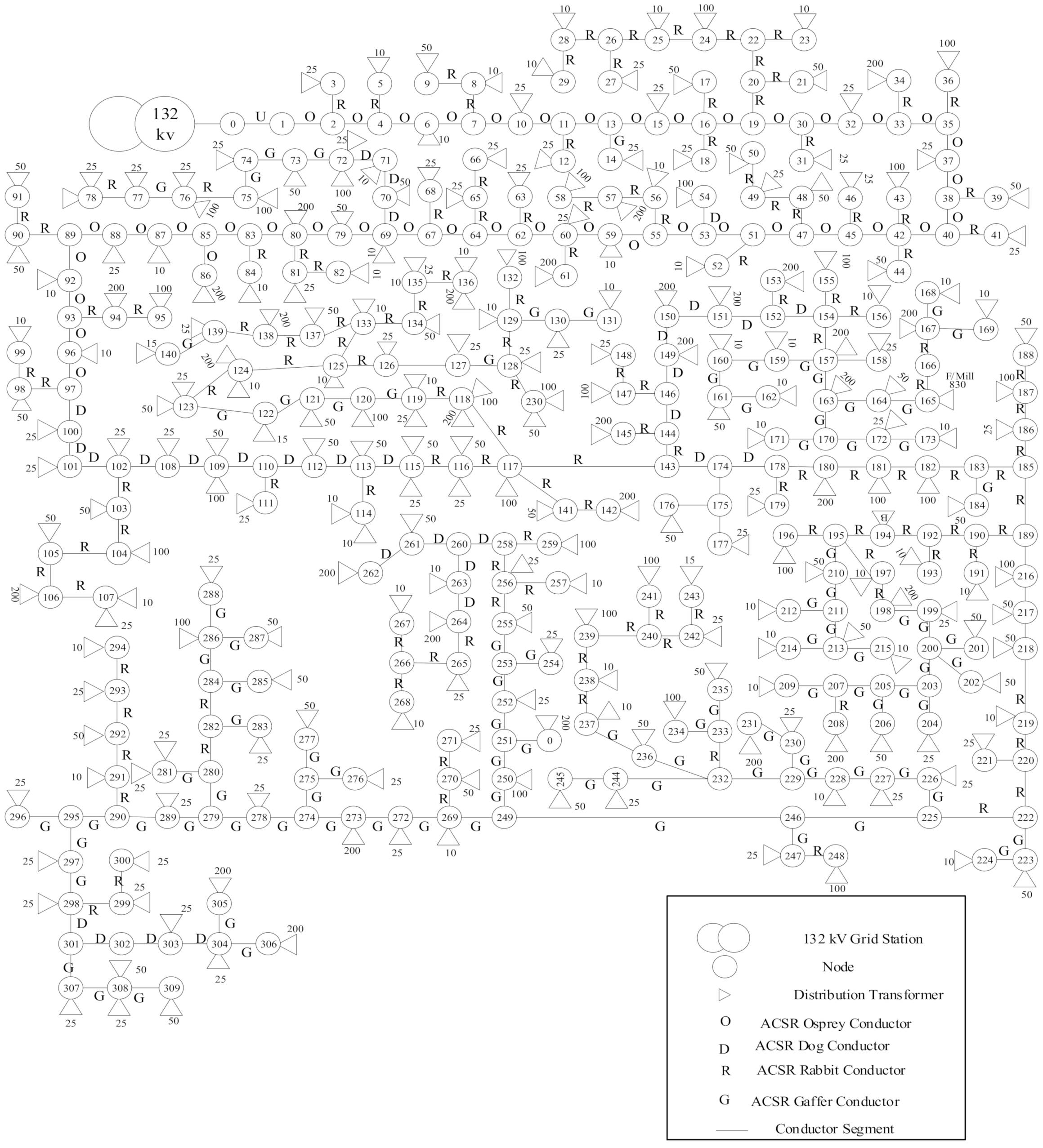
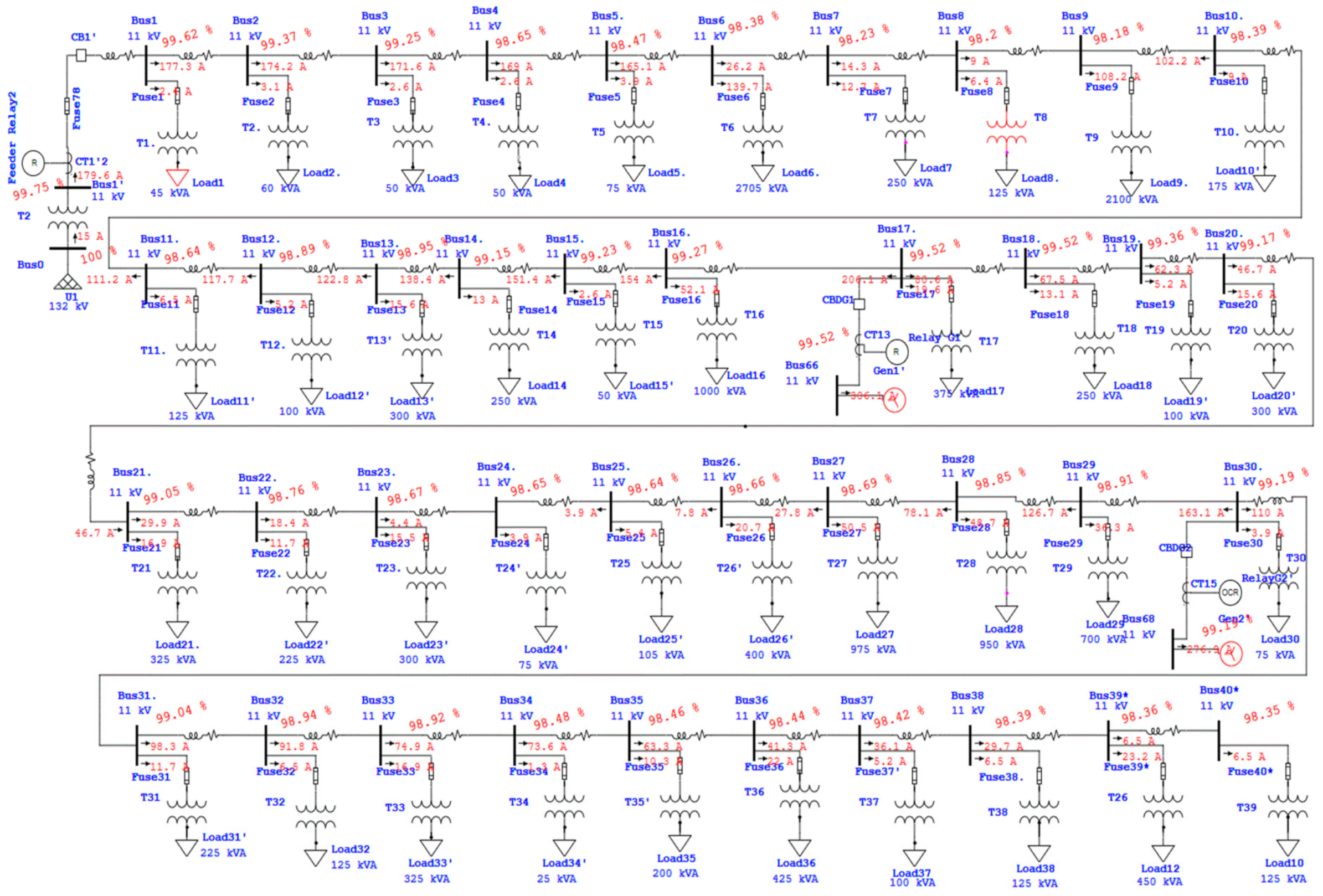
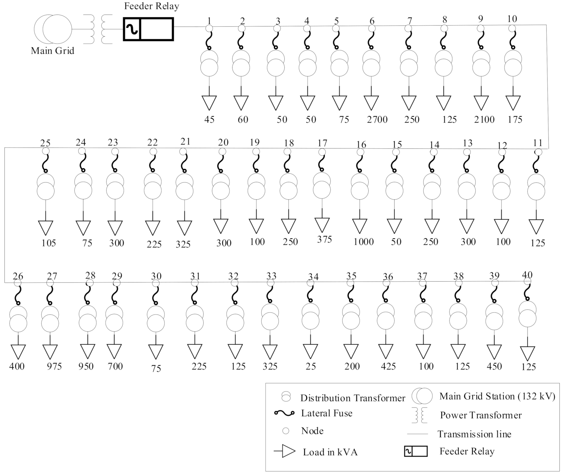
The voltage at each bus of distribution feeders must be within reference voltage ± 5% according to IEEE standards. General procedures to find optimal placement and sizes of DGs merely rely on permissible voltage limits while neglecting the accumulative power loss of the DN. In the proposed technique, we aim to find a solution in which all buses have acceptable voltages with minimum possible deviation from nominal values and minimum accumulative power loss.

To meet the stated objective, we have devised a PSO-based technique. PSO is a bird flocking and fish schooling influential optimization approach based on population, helpful in optimizing complex multidimensional problems. The algorithm initiates a population of swarm particles with assigned random velocity and position. Each swarm particle represents a solution set. The swarm particles moved in the search space to fulfill the requirements of objective function while satisfying constraints. Each particle must be evaluated by the output of the objective function against the fitness value by using a load flow algorithm. In each iteration, particles update their velocity to have a better solution according to the best-fit particle. Identifying the best-fit particle, if local fitness ($p)$ gives better results than the current best ($pbest$) value, then replaced the current fitness ($pbest$) with local fitness ($p$). If current fitness is better than the global best, then set $gbest=pbest.$ This process continues by updating the velocity and position of particles until the stopping criteria are reached, and $gbest$ will be the optimal solution.

SPSO algorithm flowchart is depicted in Figure 2. In the beginning, system parameters are loaded in the simulation system. If some system configuration file is not available, parameters of DN under consideration can be input manually. After loading the system’s parameters, values of different parameters associated with the SPSO technique such as population size, dimensions of particles and their constraint limits, number of iterations, etc. are initialized.

Then a random population of the particles is initialized with random velocity and positions. Due to the inherent nature of SPSO, these swarm particles acquire random positions in search space of selected dimension $D$ as given in (17).

S_D = [S_D1, S_D2,…, S_DN]

(17)

Here D is the dimension of search space. S_D1 is the position of particles for dimension one, S_D2 is the position of particles for dimension two, similarly, the further positions of particles up to S_DN represents the positions for remaining dimensions. In a distributed network, the number of loops formed equals the number of dimensions by closing all the tie-switches. Branches of a loop have constituted the search space of a dimension. However, the branches of the network which do not belong to any loop are not in any search space. Therefore, these branches are not considered in the optimization process. The SPSO can be applied to find the optimal solution after specifying the number of dimensions and the search space for each dimension. $DN$ denotes total selected random positions in dimension D and $S_D$ reflects its collection in dimension $D$. S_D selects the best position from the different position vectors from S_D1 to S_DN. In SPSO, the fitness function nature of the conventional PSO is replaced with logistic sigmoid function sig ($V_{iD}^{K+1}$) because respective $D$ dimensions taken from $DN$ positions are mapped with $S_D$. So, the position of respective swarms in dimension $D$ is altered from being a point in real value to selected space. The logistic sigmoid function is given by (18).

$$sig (V_{iD}^{K+1})=DN\left(\frac{1}{1+\exp \left(-V_{iD}^{K+1}\right)}\right)$$

(18)

By applying sigmoid transformation to binary PSO, the velocities are confined to range of [0,1]. It must be ensured that particle position values are either 1 or 0.

$$x_{iD}^{K+1}=\left\{\begin{array}{c}0, if \sigma \ge sig \left(V_{iD}^{K+1}\right) \\ 1, if \sigma <sig \left(V_{iD}^{K+1}\right)\end{array}\right.$$

(19)

The local and global best ($gbest$) values are updated after evaluating the fitness function. Then termination criteria regarding the number of iterations are checked at the end of each iteration. If the criteria are not met, then the positions and velocities of the particles in the swarm are updated using (20)–(22). The ith swarm position in the respective $D$dimension is updated by (20).

$$x_{iD}^{K+1}=\left\{\begin{array}{c}{S}_{D1} if sig\left(V_{iD}^{k+1}\right) < 1\\ S_{D2} if sig\left(V_{iD}^{k+1}\right) < 2\\ .\\ .\\ .\\ S_{DN} if sig\left(V_{iD}^{k+1}\right) \le DN\end{array}\right.$$

(20)

$$V_{iD}^{K+1}=\left\{\begin{array}{c}{V}_{max} if V_{iD}^{K+1}>V_{max}\\ V_{iD}^{K+1} if V_{min} \le V_{iD}^{K+1} \le V_{max}\\ V_{min} if V_{iD}^{K+1} \le V_{min}\end{array}\right.$$

(21)

V_min represents the minimum possible velocity and V_max maximum velocity. For each iteration velocity of swarms updated avoids invariability in the velocity of ith swarms, velocity is updated by (22).

$$v_{iD}^{K+1}=\left\{\begin{array}{c}rand\times V_{iD}^{K+1} if \left|V_{iD}^{K+1}\right| = \left|V_{iD}^K\right|\\ V_{iD}^{K-1} otherwise\end{array}\right.$$

(22)

The same process is repeated until the termination criteria are met. The optimal solution is the value stored in $gbest$.

4. Case Study

One 11 kV radial distribution feeder of subdivision GEPCO is used for evaluation. The considered feeder is Rajewala distribution feeder which is 120 km long and comes from 132 kV Eimnabad grid station. This feeder has 506 nodes, and it supplies a total load of 14,740 kVA including domestic, industrial, and commercial loads. Results of field inspection about various parameters of this feeder such as load at each bus, segment length, resistance, inductance, impedance, etc. are depicted in

Table 1. Line parameters of actual distribution feeder.

From Node–Node	Resistance (Ω)	Segment Length (km)	Inductive Reactance (Ω)	Impedance (Ω)	Bus Load (kVA)
0–1	0.040	0.12	0.045	0.067	45
1–2	0.079	0.235	0.088	0.119	60
2–3	0.040	0.12	0.045	0.061	50
3–4	0.205	0.609	0.230	0.308	50
4–5	0.061	0.183	0.069	0.092	75
5–6	0.033	0.098	0.037	0.049	2705
6–7	0.279	0.83	0.313	0.419	250
7–8	0.077	0.229	0.087	0.116	125
8–9	0.092	0.275	0.104	0.139	2100
9–10	0.139	0.414	0.157	0.209	175
10–11	0.157	0.466	0.177	0.236	125
11–12	0.140	0.417	0.158	0.211	100
12–13	0.031	0.091	0.034	0.046	300
13–14	0.095	0.283	0.107	0.143	250
14–15	0.034	0.101	0.039	0.051	50
15–16	0.016	0.049	0.018	0.024	1000
16–17	0.075	0.223	0.084	0.113	375
17–18	0.007	0.002	0.008	0.001	250
18–19	0.129	0.384	0.145	0.194	100
19–20	0.177	0.528	0.199	0.267	300
20–21	0.146	0.436	0.165	0.221	325
21–22	0.528	1.573	0.594	0.795	225
22–23	0.245	0.732	0.277	0.370	300
23–24	0.206	0.613	0.232	0.310	75
24–25	0.031	0.091	0.034	0.046	105
25–26	0.398	1.182	0.447	0.597	400
26–27	0.072	0.214	0.081	0.108	975
27–28	0.135	0.402	0.152	0.203	950
28–29	0.030	0.09	0.034	0.045	700
29–30	0.108	0.32	0.121	0.161	75
30–31	0.139	0.412	0.1557	0.208	225
31–32	0.031	0.091	0.0344	0.046	125
32–33	0.108	0.32	0.121	0.162	325
33–34	0.163	0.488	0.1845	0.247	25
34–35	0.043	0.127	0.048	0.064	200
35–36	0.246	0.732	0.277	0.370	425
36–37	0.278	0.828	0.313	0.418	100
37–38	0.492	1.464	0.553	0.740	125
38–39	0.134	0.399	0.151	0.202	450
39–40	0.061	0.183	0.069	0.093	125

. A one-line diagram of the original feeder based on the field survey is given in Figure 3. For illustration, the distribution feeder is divided into small segments within the specified nodes.

Accumulating inspection data, 506 nodes are compressed to 40 nodes as depicted in the simplified diagram shown in Figure 4. It is perceived that generalization of the feeder’s data will not have any influence on outcomes. The same calculations can be prepared on actual data without generalizing it to acquire approximately identical results. The only difference will be that calculations will grow complex and longer.

The SPSO algorithm proceeds through all possible iterations. SPSO parameters such as swarm = 500, number of iterations = 3000, W_min = 0.4, W_max = 0.9 are the inertia weights. SPSO simulation is performed using MATLAB R2018Ra installed on a personnel computer with Intel Core i5-4200u processor, 1.60 GHz, 4GB RAM, x64-bit based Windows platform. The results obtained through MATLAB are also verified through ETAP.

5. Simulation Results and Discussion

Different simulation cases are carried out on a simplified real distribution feeder, and a comparison is made among the output results of all cases in order to validate the effectiveness of the proposed SPSO approach. Simulated cases are the following:

• Evaluation of objective parameters without DGs
• Evaluation of objective parameters with DGs through SPSO
• Evaluation of objective parameters with DGs through ETAP
• Comparison of proposed SPSO outcomes with other approaches

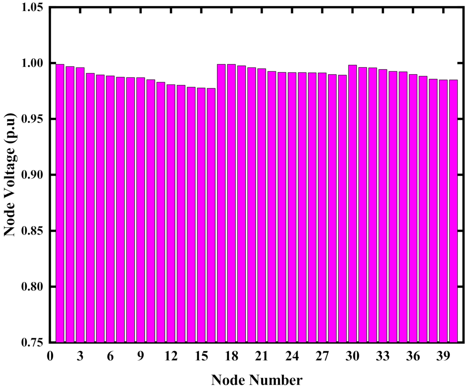
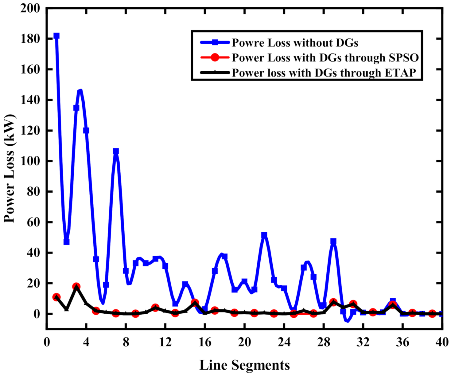
5.1. Evaluation of Objective Parameters without DGS

In this section, the load flow analysis is presented without DGs with the actual feeder parameters. The objective func tion values are calculated, which are then compared with the objective function values when DGs will be connected with the distribution feeder later on. The feeder retains its inherent radial nature, with current flowing in a single direction from the primary source end to the load. Without the intrusion of DGs and the network is passive. The objective of this experiment is to show that the node voltages violate the permissible limits in the case of a sole grid source supplying a whole load of a lengthy feeder with a non-uniform load growth nature. This experiment also shows that the accumulative power loss is high without DGs.

Table 2. Load flow results For DN without DG.

Sr. No	From Node–Node	Segment Currents (A)	Segment Voltage Drops (V)	Node Voltage at Receiving End (p.u.)	Power Loss (kW)
1	0–1	773.649	46.952	0.995	182.002
2	1–2	771.287	91.667	0.987	46.972
3	2–3	768.138	46.618	0.983	134.812
4	3–4	765.514	235.778	0.962	119.912
5	4–5	762.889	70.606	0.955	35.786
6	5–6	758.953	37.616	0.952	18.967
7	6–7	617.953	259.398	0.928	106.495
8	7–8	604.832	70.049	0.922	28.147
9	8–9	598.271	83.207	0.914	33.073
10	9–10	488.271	102.233	0.905	33.163
11	10–11	479.085	112.091	0.895	35.937
12	11–12	472.524	99.654	0.886	31.284
13	12–13	467.276	21.505	0.884	6.676
14	13–14	451.530	64.625	0.877	19.386
15	14–15	438.408	22.394	0.876	6.523
16	15–16	435.784	10.799	0.875	3.126
17	16–17	383.298	43.228	0.871	28.038
18	17–18	363.615	0.368	0.871	37.450
19	18–19	350.494	68.068	0.865	15.850
20	19–20	345.245	92.192	0.856	21.146
21	20–21	329.499	72.656	0.849	15.905
22	21–22	312.441	248.559	0.827	51.595
23	22–23	300.632	111.296	0.817	22.229
24	23–24	284.886	88.321	0.809	16.716
25	24–25	281.496	12.955	0.808	2.423
26	25–26	275.986	164.982	0.792	30.250
27	26–27	254.992	27.597	0.790	24.182
28	27–28	203.892	41.453	0.785	5.615
29	28–29	154.029	7.011	0.786	47.534
30	29–30	117.329	18.988	0.784	1.480
31	30–31	113.393	23.627	0.781	1.266
32	31–32	101.593	4.675	0.782	0.934
33	32–33	95.032	15.379	0.780	0.971
34	33–34	78.032	19.258	0.778	0.998
35	34–35	76.719	4.927	0.778	8.201
36	35–36	66.223	24.516	0.775	0.069
37	36–37	43.915	18.390	0.774	0.536
38	37–38	38.667	28.629	0.772	0.137
39	38–39	32.107	6.478	0.770	0.138
40	39–40	8.488	0.785	0.771	0.004
Total Voltage Drop = 2520.365 V			Total Power Loss = 1175.935 kW

shows the load flow analysis results and objective function values. It shows that without DGs’ integration, the voltages within limits are confined to the first 10 buses near to source end. After that, the voltage starts dipping to lower limits. This decrease in node voltages prevails to the last node 40 where the minimum voltage 0.77 p.u. is observed. Total voltage drops and power loss in the network are 2520.365 V and 1175.935 kW correspondingly in this case. The per-unit value of the bus voltage is shown in Figure 5.

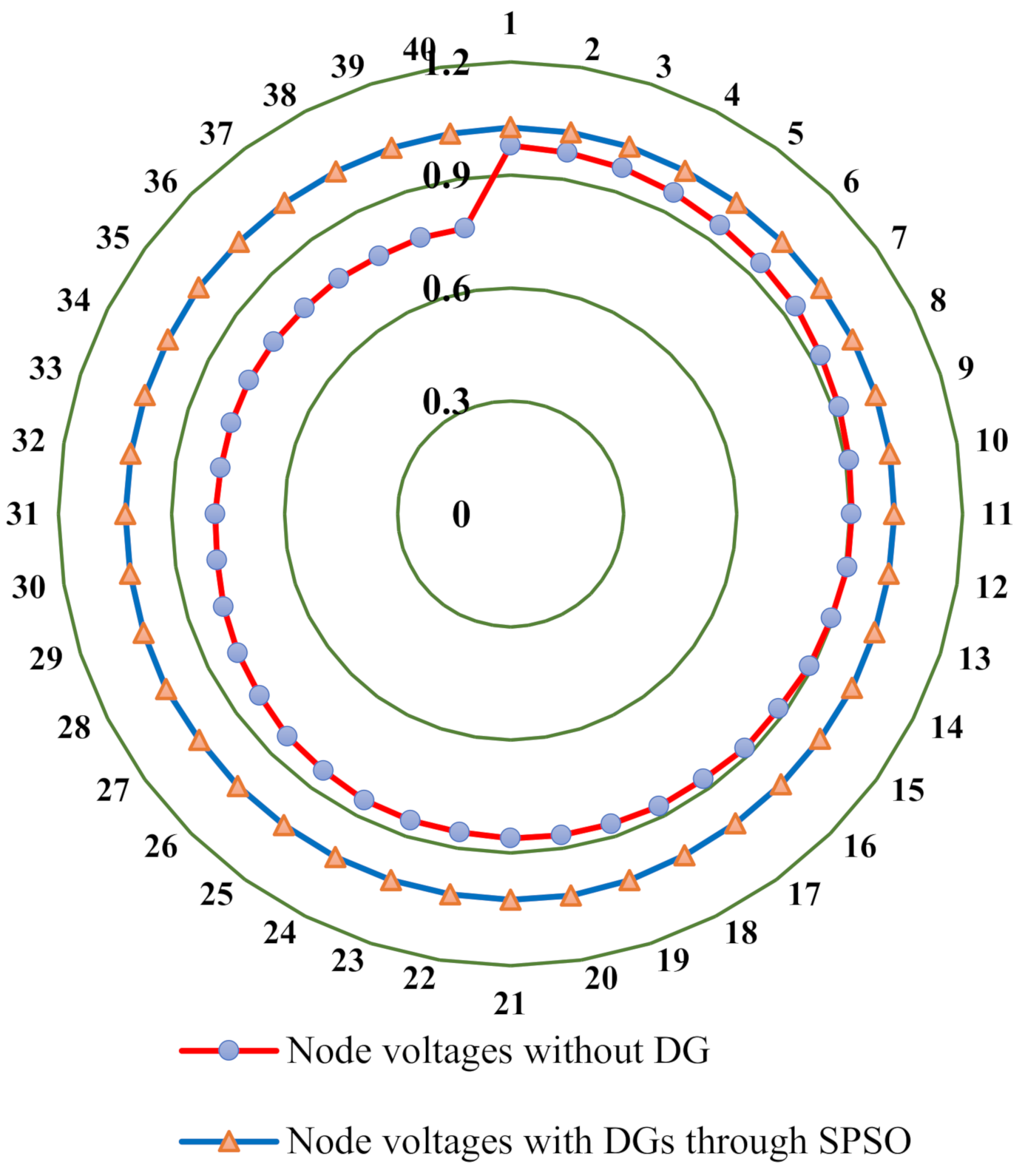
5.2. Evaluation of Objective Parameters with DGs through SPSO

In this section, the effective optimal DG application is carried out through SPSO. The objective of this simulation is to reduce the accumulative power loss in the system and voltage profile improvement by integrating DGs through the proposed technique. Node voltages in per-unit (p.u.) values are shown in Figure 6.

SPSO parameters are such as swarm particles and iterations (K) are 500 and 3000, minimum and maximum acceleration factors are 0.4 and 0.9, respectively. Two DGs are decided to be connected with the distribution feeder. Equations (1)–(14) provide objective functions and constraints. MATLAB R2018a is employed for algorithm simulations. Figure 7 shows the convergence process of SPSO.

After running the algorithm, the optimal positions obtained for DG1 and DG2 are at bus numbers 17 and 30, respectively. The optimal sizes for DG1 and DG2 are 5802 kVA and 5232 kVA, respectively.

Table 3. Load flow results for DN with DGs through SPSO.

Sr. No.	From Node–Node	Segment Currents (A)	Segment Voltage Drops (V)	Node Voltage at Receiving End (p.u.)	Power Loss (kW)
1	0–1	188.749	11.455	0.998	10.856
2	1–2	186.387	22.152	0.996	2.748
3	2–3	183.238	11.120	0.995	17.783
4	3–4	180.614	55.629	0.990	6.689
5	4–5	177.989	16.473	0.989	1.953
6	5–6	174.053	8.626	0.988	0.999
7	6–7	33.053	13.874	0.987	0.308
8	7–8	19.931	2.308	0.987	0.031
9	8–9	13.370	1.859	0.987	0.053
10	9–10	96.629	20.232	0.985	0.921
11	10–11	105.814	24.938	0.983	3.977
12	11–12	112.375	23.699	0.981	1.763
13	12–13	117.624	5.413	0.981	0.421
14	13–14	133.037	19.088	0.978	1.686
15	14–15	146.491	7.482	0.978	7.189
16	15–16	149.116	3.695	0.977	0.365
17	16–17	105.598	11.909	0.998	2.176
18	17–18	85.916	0.086	0.998	2.149
19	18–19	72.794	14.137	0.997	0.706
20	19–20	67.545	18.036	0.996	0.838
21	20–21	51.799	11.422	0.994	0.411
22	21–22	34.742	27.638	0.992	0.682
23	22–23	22.932	8.489	0.993	0.259
24	23–24	7.186	2.227	0.992	0.028
25	24–25	3.796	0.174	0.992	0.008
26	25–26	1.713	1.024	0.991	0.001
27	26–27	22.709	2.457	0.991	0.172
28	27–28	73.809	15.006	0.989	0.712
29	28–29	123.671	5.629	0.989	7.553
30	29–30	117.329	18.988	0.998	4.233
31	30–31	113.393	23.627	0.996	6.408
32	31–32	101.592	4.675	0.998	0.934
33	32–33	95.032	15.379	0.994	0.971
34	33–34	78.032	19.258	0.992	0.998
35	34–35	76.719	4.927	0.992	5.847
36	35–36	66.222	24.516	0.989	0.069
37	36–37	43.916	18.390	0.988	0.536
38	37–38	38.667	28.629	0.986	0.137
39	38–39	32.106	6.478	0.985	0.138
40	39–40	8.488	0.785	0.984	0.004
Total Voltage Drop = 531.929 V			Total Power Loss = 92.44 kW

shows the objective function values obtained by these optimal positions and sizes of DGs after load flow analysis. With the effective implementation of DGs through the proposed SPSO, the voltages at all the nodes are now within the standard limits, and accumulative power loss is considerably reduced from 1175.935 kW to 92.444 kW. The supply from the main power grid is reduced due to the handling of excessive load by DG. Due to which less current flows in transmission lines, resulting in reduced active power loss and voltage drop. The optimal results are achieved when DGs are integrated at accurate positions.

5.3. Evaluation of Objective Parameters with DGs through ETAP

In this section simulations to validate the use of SPSO algorithm to find the positions for distributed generators are presented. The actual feeder circuit is simulated in ETAP software and DGs are connected at the optimal location with optimal size obtained from SPSO. Figure 8 shows the load flow analysis by using ETAP. This figure represents the node voltages as the percentage of nominal voltage (11 kV) in red color at each node. It can be visualized that these node voltages are within limits. Load flow analysis is conducted and obtained results through ETAP are given in

Table 4. Load flow results for DN with optimal DGs through ETAP.

Sr. No.	From Node–Node	Segment Currents (A)	Segment Voltage Drops (V)	Node Voltage at Receiving End (p.u.)	Power Loss (kW)
1	0–1	188.949	11.467	0.996	10.856
2	1–2	186.587	22.176	0.995	2.748
3	2–3	183.438	11.132	0.990	17.783
4	3–4	180.813	55.690	0.989	6.689
5	4–5	178.189	16.491	0.988	1.952
6	5–6	174.253	8.636	0.987	0.999
7	6–7	33.253	13.958	0.987	0.308
8	7–8	20.131	2.331	0.986	0.032
9	8–9	13.570	1.887	0.985	0.053
10	9–10	96.429	20.190	0.982	0.922
11	10–11	105.614	24.890	0.980	3.977
12	11–12	112.175	23.657	0.980	1.763
13	12–13	117.423	5.404	0.978	0.422
14	13–14	133.169	19.060	0.977	1.686
15	14–15	146.291	7.472	0.977	7.189
16	15–16	148.915	3.690	0.998	0.365
17	16–17	104.998	11.841	0.998	2.104
18	17–18	85.315	0.862	0.997	2.061
19	18–19	72.194	14.020	0.996	0.673
20	19–20	66.945	17.876	0.995	0.796
21	20–21	51.199	11.289	0.992	0.384
22	21–22	34.141	27.160	0.992	0.616
23	22–23	22.331	8.267	0.991	0.223
24	23–24	6.586	2.041	0.992	0.018
25	24–25	3.196	0.147	0.991	0.312
26	25–26	2.313	1.383	0.991	0.021
27	26–27	23.308	2.522	0.988	0.202
28	27–28	74.408	15.128	0.989	0.747
29	28–29	124.270	5.656	0.998	7.776
30	29–30	117.329	18.988	0.996	4.233
31	30–31	113.392	23.627	0.996	6.408
32	31–32	101.592	4.675	0.994	0.935
33	32–33	95.032	15.379	0.993	0.972
34	33–34	78.032	19.258	0.992	0.998
35	34–35	76.719	4.927	0.989	5.847
36	35–36	66.222	24.516	0.988	0.069
37	36–37	43.915	18.390	0.985	0.536
38	37–38	38.667	28.629	0.985	0.137
39	38–39	32.106	6.478	0.985	0.138
40	39–40	8.487	0.785	0.997	0.443
Total Voltage Drop = 550.975			Total Power Loss = 93.996 kW

. The total voltage drops, and power losses are 531.975 V and 93.720 kW, respectively. The outcomes are identical to results through SPSO implemented in MATLAB R2018a, which validate the effectiveness of the proposed technique for DG integration.

Comprehensive comparisons among the accumulative power loss and voltage drop without DG, with DGs through SPSO and ETAP are given in Figure 9 and Figure 10, respectively. Percentage reductions in power loss and voltage drop are given in

Table 5. Accumulative voltage drops and power loss comparison in different situations.

	Total Voltage Drops (V)	Total Power Loss (kW)	Reduction in Voltage Drops	Reduction in Power Loss
Without DGs	2520.365	1175.935
With DGs through SPSO	531.929	92.44	78.89%	92.139%
With DGs through ETAP	550.975	93.996	78.13%	92.006%

. Figure 9 and Figure 10 show a significant improvement in voltage profile at each node with power loss reduction.

The experiment proves that the devised technique for the effective implementation of multiple DG sources under extreme load growth conditions worked efficiently.

5.4. Comparison of Proposed SPSO Outcomes with Other Approaches

In this section, the proposed SPSO algorithm for optimal DGs location has been compared with other approaches in the literature. It has been observed that SPSO algorithm optimal DGs size as compared to ABC optimization algorithm, crow search optimization algorithm (CSOA), polar bear optimization algorithm (PBOA), GA-PSO and discrete PSO (DPSO). It has been analyzed that CSOA and BPOA have given lower active power loss of about 95.80 kW and 97.10 kW, respectively. In contrast, the highest active power loss has been noticed for ABC and PSO-GA that are 105.54 kW and 101.15 kW, respectively. In addition, for reactive power loss, CSOA and PSO-GA have given lower values of about 112.572 kVAR and 115.594 kVAR, respectively. In comparison, the highest reactive power loss has been observed in DPSO and ABC, which are about 128.077 kVAR and 119.054 kVAR, respectively. However, the proposed SPSO approach gives a lower active power loss of 94.44 kW and a reactive power loss of about 109.615 kVAR. Furthermore, each method has been run for 100 times to observe the computational efficiency. The DGs optimal size with location, active power loss, reactive power loss and different computational time indicators for different methods have been summarized in

Table 6. Comparison of SPSO with other approaches in terms of different outcomes.

Approach	Optimal Size (kVA)/Location (Bus No).	Active Power Loss PL (kW)	PL Reduction (%)	Reactive Power Loss QL (kVAR)	QL Reduction (%)	Vmin/ (Bus No).	Execution Time (s)
Base Case		1175.935		987.159
ABC [19]	5125/19 3503/30	105.54	91.025	119.054	87.8905	0.987/15	145.78
CSOA [48]	5518/17 5128/30	95.80	91.853	112.572	88.59637	0.989/15	224.76
BPOA [25]	5274/17 4804/30	97.10	91.743	117.847	88.0572	0.983/15	103.98
PSO-GA [49]	5880/17 4864/30	101.15	91.398	115.594	88.290	0.981/15	92.08
DPSO [44]	5516/17 5126/30	98.208	91.649	128.077	86.955	0.979/15	82.78
Proposed SPSO	5802/17 5232/30	94.044	91.969	109.615	88.896	0.991/15	40.06

. It has been explored that the execution time taken by SPSO has the lowest value of 40.06 sec compared to other approaches, which confirms the proposed strategy is computationally reasonable.

6. Conclusions

Optimum siting of properly sized DGs in DNs can resolve their various operational issues. On the other side, inappropriate sizing and siting can magnify voltage drops and power loss. In this work, an SPSO-based algorithm is proposed for the optimal sizing and placement of multiple DGs in DN. The node voltages can violate the permissible limits without proper DG placement. After integrating optimal DGs, the voltage profile is significantly improved, and all the node voltages remain within limits. About 78% reduction in accumulated voltage drop in the system’s branches is observed as compared to the case where no DG is connected. The results are confirmed by ETAP as well. It is observed that active power loss with DGs is reduced by 92%. Initializing DGs lessens the current from the main source; therefore, voltage drop, and power loss are also declined. Installation of RER-based DGs can be beneficial for both electric utilities and consumers compared to fossil fuel-based sources. These support generation, transmission, and distribution systems cost-effectively in an eco-friendly manner. Their optimal installment is of considerable importance for energy management in smart cities. In the future, the integration of wind and PV in the existing power system can be observed with various load control mechanisms. Different protection schemes and the impact of transients in the power system can be explored. Furthermore, the demand side flexibility can be computed to initiate demand response actions in the power system integrated with DGs.

References

1. Popa, G.N.; Iagăr, A.; Diniș, C.M. Considerations on Current and Voltage Unbalance of Nonlinear Loads in Residential and Educational Sectors. Energies 2021, 14, 102. [Google Scholar] [CrossRef]
2. Bayatloo, F.; Bozorgi-Amiri, A. A novel optimization model for dynamic power grid design and expansion planning considering renewable resources. J. Clean. Prod. 2019, 229, 1319–1334. [Google Scholar] [CrossRef]
3. Ameli, A.; Bahrami, S.; Khazaeli, F.; Haghifam, M. A Multiobjective Particle Swarm Optimization for Sizing and Placement of DGs from DG Owner’s and Distribution Company’s Viewpoints. IEEE Trans. Power Deliv. 2014, 29, 1831–1840. [Google Scholar] [CrossRef]
4. Rizwan, M.; Hong, L.; Waseem, M.; Shu, W. Sustainable protection coordination in presence of distributed generation with distributed network. Int. Trans. Electr. Energy Syst. 2020, 30, e12217. [Google Scholar] [CrossRef]
5. Gampa, S.R.; Das, D. Optimum placement and sizing of DGs considering average hourly variations of load. Int. J. Electr. Power Energy Syst. 2015, 66, 25–40. [Google Scholar] [CrossRef]
6. Hu, X.; Zhou, H.; Liu, Z.; Yu, X.; Li, C. Hierarchical Distributed Scheme for Demand Estimation and Power Reallocation in a Future Power Grid. IEEE Trans. Ind. Inform. 2017, 13, 2279–2290. [Google Scholar] [CrossRef]
7. Khalid, M.; Akram, U.; Shafiq, S. Optimal Planning of Multiple Distributed Generating Units and Storage in Active Distribution Networks. IEEE Access 2018, 6, 55234–55244. [Google Scholar] [CrossRef]
8. El-Fergany, A. Optimal allocation of multi-type distributed generators using backtracking search optimization algorithm. Int. J. Electr. Power Energy Syst. 2015, 64, 1197–1205. [Google Scholar] [CrossRef]
9. Alshehri, J.; Khalid, M. Power quality improvement in microgrids under critical disturbances using an intelligent decoupled control strategy based on battery energy storage system. IEEE Access 2019, 7, 147314–147326. [Google Scholar] [CrossRef]
10. Yin, F.; Hajjiah, A.; Jermsittiparsert, K.; Al-Sumaiti, A.S.; Elsayed, S.K.; Ghoneim, S.S.M.; Mohamed, M.A. A Secured Social-Economic Framework Based on PEM-Blockchain for Optimal Scheduling of Reconfigurable Interconnected Microgrids. IEEE Access 2021, 9, 40797–40810. [Google Scholar] [CrossRef]
11. Paiva, S.; Ahad, M.A.; Tripathi, G.; Feroz, N.; Casalino, G. Enabling Technologies for Urban Smart Mobility: Recent Trends, Opportunities and Challenges. Sensors 2021, 21, 2143. [Google Scholar] [CrossRef]
12. Ahad, M.A.; Biswas, R. Request-based, secured and energy-efficient (RBSEE) architecture for handling IoT big data. J. Inf. Sci. 2019, 45, 227–238. [Google Scholar] [CrossRef]
13. Iqbal, M.M.; Sajjad, I.A.; Manan, A.; Waseem, M.; Ali, A.; Sohail, A. Towards an Optimal Residential Home Energy Management in Presence of PV Generation, Energy Storage and Home to Grid Energy Exchange Framework. In Proceedings of the 2020 3rd International Conference on Computing, Mathematics and Engineering Technologies (iCoMET), Sukkur, Pakistan, 29–30 January 2020; pp. 1–7. [Google Scholar]
14. Grubic, T.; Varga, L.; Hu, Y.; Tewari, A. Micro-generation technologies and consumption of resources: A complex systems’ exploration. J. Clean. Prod. 2020, 247, 119091. [Google Scholar] [CrossRef]
15. Rizwan, M.; Hong, L.; Waseem, M.; Sharaf, M.; Shafiq, M. A Robust Adaptive Overcurrent Relay Coordination Scheme for Wind-Farm-Integrated Power Systems Based on Forecasting the Wind Dynamics for Smart Energy Systems. Appl. Sci. 2020, 10, 6318. [Google Scholar] [CrossRef]
16. Waseem, M.; Sajjad, I.A.; Napoli, R.; Chicco, G. Seasonal Effect on the Flexibility Assessment of Electrical Demand. In Proceedings of the 2018 53rd International Universities Power Engineering Conference (UPEC), Glasgow, UK, 4–7 September 2018; pp. 1–6. [Google Scholar]
17. Waseem, M.; Sajjad, I.A.; Haroon, S.S.; Amin, S.; Farooq, H.; Martirano, L.; Napoli, R. Electrical Demand and its Flexibility in Different Energy Sectors. Electr. Power Compon. Syst. 2020, 48, 1339–1361. [Google Scholar] [CrossRef]
18. Ma, M.; Zhang, C.; Liu, X.; Chen, H. Distributed Model Predictive Load Frequency Control of the Multi-Area Power System After Deregulation. IEEE Trans. Ind. Electron. 2017, 64, 5129–5139. [Google Scholar] [CrossRef]
19. Mohandas, N.; Balamurugan, R.; Lakshminarasimman, L. Optimal location and sizing of real power DG units to improve the voltage stability in the distribution system using ABC algorithm united with chaos. Int. J. Electr. Power Energy Syst. 2015, 66, 41–52. [Google Scholar] [CrossRef]
20. Waseem, M.; Lin, Z.; Liu, S.; Zhang, Z.; Aziz, T.; Khan, D. Fuzzy compromised solution-based novel home appliances scheduling and demand response with optimal dispatch of distributed energy resources. Appl. Energy 2021, 290, 116761. [Google Scholar] [CrossRef]
21. Suchitra, D.; Jegatheesan, R.; Deepika, T.J. Optimal design of hybrid power generation system and its integration in the distribution network. Int. J. Electr. Power Energy Syst. 2016, 82, 136–149. [Google Scholar] [CrossRef]
22. Mohamed, M.A.; Abdullah, H.M.; El-Meligy, M.A.; Sharaf, M.; Soliman, A.T.; Hajjiah, A. A novel fuzzy cloud stochastic framework for energy management of renewable microgrids based on maximum deployment of electric vehicles. Int. J. Electr. Power Energy Syst. 2021, 129, 106845. [Google Scholar] [CrossRef]
23. Jain, S.; Kalambe, S.; Agnihotri, G.; Mishra, A. Distributed generation deployment: State-of-the-art of distribution system planning in sustainable era. Renew. Sustain. Energy Rev. 2017, 77, 363–385. [Google Scholar] [CrossRef]
24. Farh, H.M.H.; Al-Shaalan, A.M.; Eltamaly, A.M.; Al-Shamma’A, A.A. A Novel Crow Search Algorithm Auto-Drive PSO for Optimal Allocation and Sizing of Renewable Distributed Generation. IEEE Access 2020, 8, 27807–27820. [Google Scholar] [CrossRef]
25. Fayyaz, S.; Sattar, M.K.; Waseem, M.; Ashraf, M.U.; Ahmad, A.; Hussain, H.A.; Alsubhi, K. Solution of Combined Economic Emission Dispatch Problem Using Improved and Chaotic Population-Based Polar Bear Optimization Algorithm. IEEE Access 2021, 9, 56152–56167. [Google Scholar] [CrossRef]
26. Viral, R.; Khatod, D.K. An analytical approach for sizing and siting of DGs in balanced radial distribution networks for loss minimization. Int. J. Electr. Power Energy Syst. 2015, 67, 191–201. [Google Scholar] [CrossRef]
27. Bazmi, A.A.; Zahedi, G.; Hashim, H. Design of decentralized biopower generation and distribution system for developing countries. J. Clean. Prod. 2015, 86, 209–220. [Google Scholar] [CrossRef]
28. Hung, D.Q.; Mithulananthan, N.; Lee, K.Y. Determining PV Penetration for Distribution Systems With Time-Varying Load Models. IEEE Trans. Power Syst. 2014, 29, 3048–3057. [Google Scholar] [CrossRef]
29. Khan, H.; Choudhry, M.A. Implementation of Distributed Generation (IDG) algorithm for performance enhancement of distribution feeder under extreme load growth. Int. J. Electr. Power Energy Syst. 2010, 32, 985–997. [Google Scholar] [CrossRef]
30. Chiradeja, P.; Ramakumar, R. An approach to quantify the technical benefits of distributed generation. IEEE Trans. Energy Convers. 2004, 19, 764–773. [Google Scholar] [CrossRef]
31. Waseem, M.; Lin, Z.; Lin, Z.; Liu, S. Optimal GWCSO-based home appliances scheduling for demand response considering end-users comfort. Electr. Power Syst. Res. 2020, 187, 106477. [Google Scholar] [CrossRef]
32. Abdmouleh, Z.; Gastli, A.; Ben-Brahim, L.; Haouari, M.; Al-Emadi, N.A. Review of optimization techniques applied for the integration of distributed generation from renewable energy sources. Renew. Energy 2017, 113, 266–280. [Google Scholar] [CrossRef]
33. Aziz, T.; Lin, Z.; Waseem, M.; Liu, S. Review on optimization methodologies in transmission network reconfiguration of power systems for grid resilience. Int. Trans. Electr. Energy Syst. 2021, 31, e12704. [Google Scholar] [CrossRef]
34. Ganguly, S.; Samajpati, D. Distributed Generation Allocation on Radial Distribution Networks Under Uncertainties of Load and Generation Using Genetic Algorithm. IEEE Trans. Sustain. Energy 2015, 6, 688–697. [Google Scholar] [CrossRef]
35. Vatani, M.; Alkaran, D.S.; Sanjari, M.J.; Gharehpetian, G.B. Multiple distributed generation units allocation in distribution network for loss reduction based on a combination of analytical and genetic algorithm methods. IET Gener. Transm. Distrib. 2016, 10, 66–72. [Google Scholar] [CrossRef]
36. Sheng, W.; Liu, K.-Y.; Liu, Y.; Meng, X.; Li, Y. Optimal placement and sizing of distributed generation via an improved nondominated sorting genetic algorithm II. IEEE Trans. Power Deliv. 2014, 30, 569–578. [Google Scholar] [CrossRef]
37. Azeem, O.; Ali, M.; Abbas, G.; Uzair, M.; Qahmash, A.; Algarni, A.; Hussain, M.R. A Comprehensive Review on Integration Challenges, Optimization Techniques and Control Strategies of Hybrid AC/DC Microgrid. Appl. Sci. 2021, 11, 6242. [Google Scholar] [CrossRef]
38. Zhou, Z.; Li, F.; Abawajy, J.H.; Gao, C. Improved PSO Algorithm Integrated With Opposition-Based Learning and Tentative Perception in Networked Data Centres. IEEE Access 2020, 8, 55872–55880. [Google Scholar] [CrossRef]
39. Rosa, W.d.; Gerez, C.; Belati, E. Optimal Distributed Generation Allocating Using Particle Swarm Optimization and Linearized AC Load Flow. IEEE Latin Am. Trans. 2018, 16, 2665–2670. [Google Scholar] [CrossRef]
40. Abbas, G.; Gu, J.; Farooq, U.; Asad, M.U.; El-Hawary, M. Solution of an economic dispatch problem through particle swarm optimization: A detailed survey-part I. IEEE Access 2017, 5, 15105–15141. [Google Scholar] [CrossRef]
41. Moradi, M.H.; Abedini, M.; Hosseinian, S.M. A Combination of Evolutionary Algorithm and Game Theory for Optimal Location and Operation of DG from DG Owner Standpoints. IEEE Trans. Smart Grid 2016, 7, 608–616. [Google Scholar] [CrossRef]
42. Barati, F.; Jadid, S.; Zangeneh, A. A new approach for DG planning at the viewpoint of the independent DG investor, a case study of Iran. Int. Trans. Electr. Energy Syst. 2017, 27, e2319. [Google Scholar] [CrossRef]
43. Singh, B.; Mishra, D.K. A survey on enhancement of power system performances by optimally placed DG in distribution networks. Energy Rep. 2018, 4, 129–158. [Google Scholar] [CrossRef]
44. Gomez-Gonzalez, M.; López, A.; Jurado, F. Optimization of distributed generation systems using a new discrete PSO and OPF. Electr. Power Syst. Res. 2012, 84, 174–180. [Google Scholar] [CrossRef]
45. Pesaran, H.A.M.; Huy, P.D.; Ramachandaramurthy, V.K. A review of the optimal allocation of distributed generation: Objectives, constraints, methods, and algorithms. Renew. Sustain. Energy Rev. 2017, 75, 293–312. [Google Scholar] [CrossRef]
46. Theo, W.L.; Lim, J.S.; Ho, W.S.; Hashim, H.; Lee, C.T. Review of distributed generation (DG) system planning and optimisation techniques: Comparison of numerical and mathematical modelling methods. Renew. Sustain. Energy Rev. 2017, 67, 531–573. [Google Scholar] [CrossRef]
47. IEEE. IEEE Recommended Practice for Interconnecting Distributed Resources with Electric Power Systems Distribution Secondary Networks. In IEEE Std 1547.6-2011; The IEEE Standards Association: Piscataway, NJ, USA, 2011; pp. 1–38. [Google Scholar] [CrossRef]
48. Waseem, M.; Kouser, F.; Waqas, A.B.; Imran, N.; Hameed, S.; Faheem, Z.B.; Liaqat, R.; Shabbir, U. CSOA-Based Residential Energy Management System in Smart Grid Considering DGs for Demand Response. In Proceedings of the 2021 International Conference on Digital Futures and Transformative Technologies (ICoDT2), Islamabad, Pakistan, 20–21 May 2021; pp. 1–6. [Google Scholar]
49. Garg, H. A hybrid PSO-GA algorithm for constrained optimization problems. Appl. Math. Comput. 2016, 274, 292–305. [Google Scholar] [CrossRef]
Figure 1. Line segment of radial DN from node I to node J .
Electronics 10 02542 g001
Figure 2. Flow chart for the devised approach.
Electronics 10 02542 g002
Figure 3. One-line diagram of actual feeder used for case study.
Electronics 10 02542 g003
Figure 4. Simplified 40 points diagram of 11 kV feeder.
Electronics 10 02542 g004
Figure 5. Node voltages without DG.
Electronics 10 02542 g005
Figure 6. Improvement in node voltages with DGs.
Electronics 10 02542 g006
Figure 7. Convergence characteristics of SPSO.
Electronics 10 02542 g007
Figure 8. Load flow analysis through ETAP.
Electronics 10 02542 g008
Figure 9. Segment voltage drops with and without DGs.
Electronics 10 02542 g009
Figure 10. Segment power loss with and without DGs.
Electronics 10 02542 g010