Using Graphics Processing Units and Compute Shaders in Real Time Multimodel Adaptive Robust Control

Abstract

Graphics processing units and video cards have seen a surge of usage in domains other than graphics computers, due to advances in hardware and software technologies; however, little uptake has been in the domain of systems engineering and real time control. This research article will demonstrate the use of video cards in multimodel adaptive robust control, using openGL and compute shaders. A software simulation will show the behavior of the adaptive robust multimodel control scheme as the target process is exposed to both parametric and structural disturbances and will show the viability of using graphics processing units in real time systems control.

1. Introduction

Adaptive-robust control [1,2,3] is a strategy used to control processes with nonlinear dynamics, as it guarantees reference tracking and rejection of disruption by reidentifying the process model and controller each time performance degradation is detected. It requires little a priori knowledge of the process and is best suited for situations where information about system dynamics is difficult to obtain or processes are subject to various types of disruptions. However, process identification and controller tuning in close loops can be difficult to implement correctly, and the mathematical complexities may lead the control system to miss the real-time sampling deadline for fast processes. In case of processes that are exposed to a many different types of disturbances repeatedly, a combination of multimodel [1,4] and adaptive robust control can be used to avoid reidentification of nominal models and tuning of robust controllers. Similar to adaptive and robust philosophies, multimodel control is an approach to dealing with perturbations and changes in the operating circumstances.

Instead of trying to tune algorithms or reidentify nominal models, multimodel control stores precalculated nominal models and controllers that match various working regimes. When perturbations occur, the change in the working regime is detected through switching algorithms. The correct controller and model to use for a specific working regime is determined through the computation of a switching criterion [5,6,7].

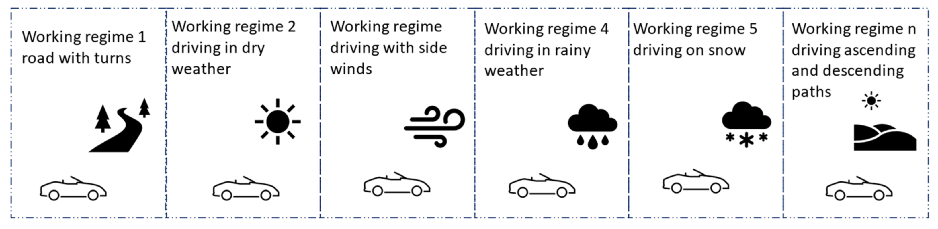
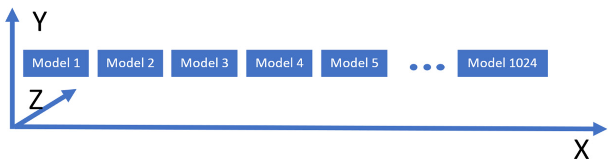
This control scheme works very well with systems that have many working regimes yet repetitive behavior. These are encountered in vehicles. One possible example is a vehicle’s suspension system, for a particular wheel. Depending on the speed, angle of movement, type of road pavement, temperature, car weight, and its weight distribution, the system behaves differently, with a different model for each working regime. Most cars tend to follow the same routes throughout their lifetime, so the repetitive nature of the perturbations is also met, as shown in Figure 1. Another example are the components of the steering system in a plane or shuttle, such as the ailerons on wings. As the plane flies through changing atmospheric conditions and executes maneuvers, the working regime of an aileron changes, accounting for multiple possible models during a single flight trip.

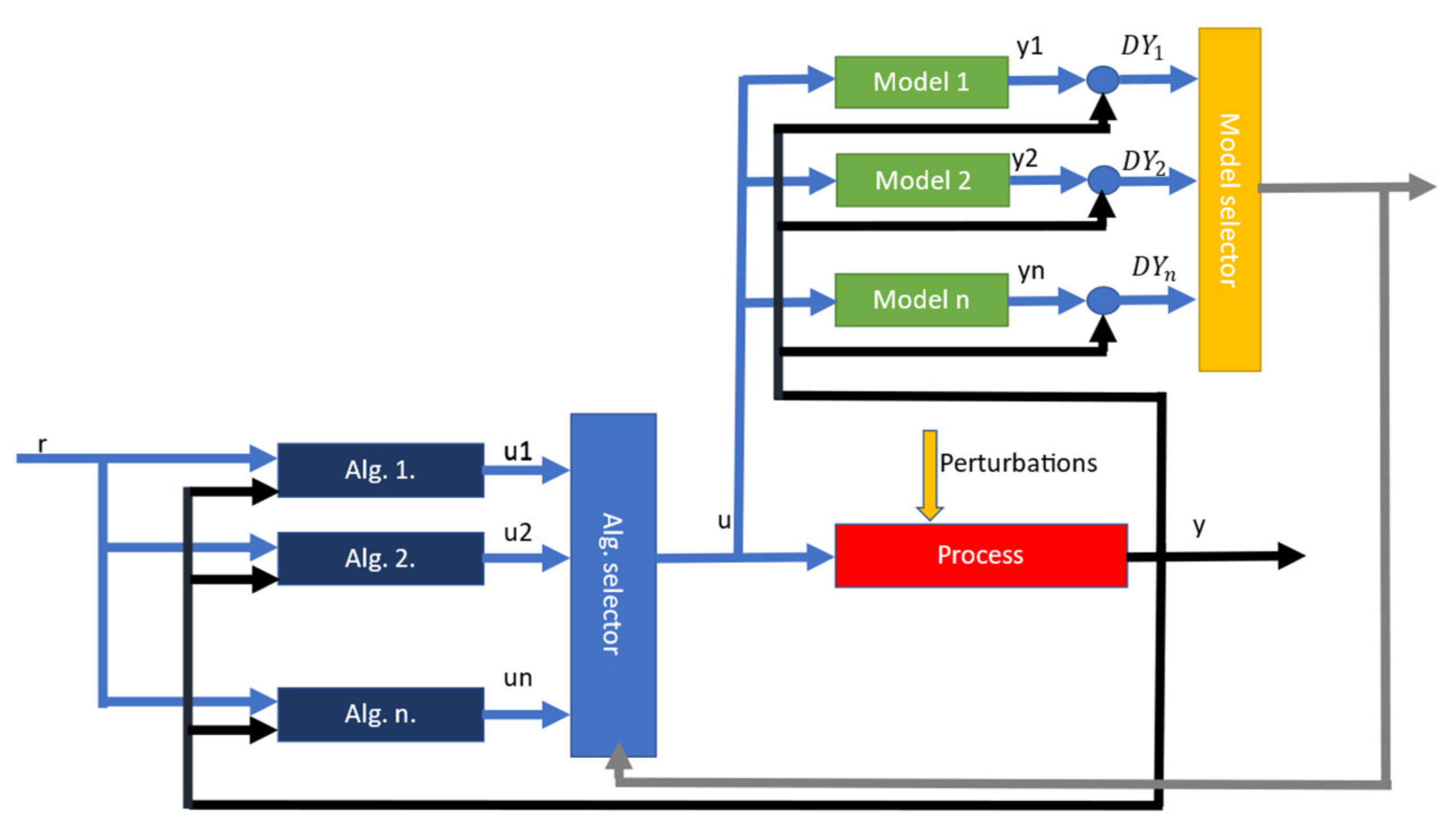
The detailed working model of the multimodel control scheme is shown in Figure 2. When the process is exposed to perturbations, either parametric or structural, the output value y changes. This output value y is then fed into the model selector block, along with the command value u. For each model in the model selector block, an output value yn is computed using the commands and the output errors of the real process. Finally,$\mathrm{yn}$, $\mathrm{u}$, $\mathrm{y}$, and $\mathrm{un}$ are used to compute a switching criterion. Based on the switching criterion, a model that best matches the real process is chosen. The switching criterion is usually based on the delta between the real process output value $\mathrm{y}$ and the output value $\mathrm{yn}$ of the nominal model [5]. With the model determined, the appropriate control algorithm is chosen from the algorithm selector block, which is then finally used to issue commands to the real process.

The multimodel part consists of a knowledge base containing previously identified nominal models and their robust controllers, matching various working regimes that are subject to different types of perturbations. Switching between the current nominal model and robust controller to one in the cache is decided by calculating a switching criterion [5], and only occurs when performance degradation is detected, a difference from the classical multimodel control philosophy, where the model switch can occur at every sampling time. If the knowledge base grows, it becomes difficult for the classical iterative approaches to compute the switching criterion for each cached nominal model and still hit the real time sampling deadline, especially when dealing with fast systems.

This article presents a novel approach to fixing the large knowledge base problem, by employing a graphics processing unit (GPU) to perform the calculation of the switching criterion in highly parallelized manner [8]. As part of this new approach, the mathematical algorithms that simulate the evolution of processes (calculation of transfer function outputs in discrete form and controller command computation) have been adapted to make full use of the particularities of the GPU hardware. A software simulation was developed to showcase the results. The software can be easily modified to work with real systems.

Other approaches so far have avoided the large knowledge base issue by limiting the number of “fixed” models and initializing an adaptive model from the initial fixed model and performing continuous tuning [9,10]. This approach is accurate but slow and is therefore unsuitable for fast processes. The proposed approach is coarse but very fast and will be better suited for fast and slow processes alike.

The paper will first present the mathematical basis of the simulation, followed by a brief explanation on how GPUs were used in the application, and finally some simulation results. The simulation results will show that the algorithms work correctly. Although the point of the research is to deal with large numbers of models, the simulation will only show four models, to better explain how it works.

2. Materials and Methods

2.1. GPU Hardware Overview

GPUs are designed to perform many mathematical operations in parallel due to the multithreaded nature of the hardware platforms, which help efficiently generate display output images, by executing a series of operations on the input data in a process called a graphics pipeline. The graphics pipeline has several stages [11] (not all mandatory—it depends on the expected results) in which various operations can be done in the outputs from of the previous stage (which become inputs for the current stage). At each stage, scripts called shaders are used to perform programmatic manipulation of input data. Among these, pixel shaders (which apply per pixel operations over a rasterized image) were typically used to perform various general purpose mathematical operations (with some limitations). In recent times, GPU hardware and driver support have evolved to expose a new kind of shader—called compute shader [12]—which can be used to perform general purpose mathematics on large data sets in a natural fashion, very similar to how things would normally operate with a classical algorithm that runs on the central processing unit (CPU) of the computer. These shaders also fully expose the parallel, heavily multithreaded nature of the GPU hardware. Compute shaders run on virtual work groups (the shader declaration defines the size of the group), composed of small execution units called cores. Each core has floating point and an integer arithmetic unit, and each core inside a virtual group has access to the same data buffers and will perform the same instructions in the same order. Virtual groups may or may not have a 1 to 1 mapping with hardware groups. In case the mapping is not exact (i.e., the size of the virtual group is not an integer multiplier of hardware group size), then the graphics hardware is not fully used, it is up to the driver and the execution scheduler in each hardware implementation to decide what happens with the unused cores in the group. Figure 3 shows an overview of nVidia Turing GPU work group (named streaming multiprocessor by Nvidia) [13].

Each core in the work group will run a thread in the compute cluster. The compute cluster represents the total number of threads assigned by the application when invoking the compute shader. When invocation occurs, the programmer can decide how many work groups will be executed as part of the compute cluster. The total number of threads will be the product of the group size, defined by the shader declaration in source code, and the total number of groups passed to the invocation call. The maximum number of threads in a compute cluster depends on the framework being used to access the GPU hardware and the hardware specifications of each GPU. Both the size of the virtual compute group and the total number of groups dispatched can be represented in 3D vector numbers, with X, Y, and Z sizes. This helps process data that are naturally 3D, but in this research, Y and Z are always 1, as the data are naturally a 1D array, so both the group size and the number of groups are effectively 1D vectors. Attempting to map it to 3D does not offer any advantages, so a design choice was made to keep Y and Z always 1 [12].

Even though compute shaders can provide support in computing various mathematical operations needed as part of the usual graphics generating pipeline, they can be used outside of the graphics pipeline to act as powerful mathematical co-processors for the applications. This feature, however, depends on the framework being used to access the hardware. DirectX allows calling compute shaders [14,15] without an actual game window; openGL currently does not. This is not a problem in itself when it comes to industrial applications. In most cases, a process computer will have some sort of user interface that is used to show the status and evolution of the process, so the requirement of an active openGL context is already met. The calling of compute shaders will be strictly tied to the refresh rate of the graphics context. This refresh rate can be coordinated with the system sampling time, to ensure real time responsiveness, when using openGL [11]. In case of DirectX, conditions are much simpler because programmers can directly access the hardware pointers and create contexts whenever it is necessary [14,15,16].

In the case of the multimodel adaptive control philosophy presented here, each core will execute the logic needed to compute the value of a switching criterion, which is then used to execute a nominal model and controller switch in the real plant. Since a GPU boosts hundreds of cores, it is quite easy to maintain a large knowledge base of nominal models and their optimal controllers and compute the switching criterion in parallel, while still adhering to the strict sampling time requirements imposed by real time control. This is not trivially possible when using just a CPU, because it lacks the number of cores that a GPU has, and it is more likely to perform these calculations in parallel [8,17].

The simulation software used in this research was developed in C#, using Visual Studio 2019, and targets the net framework 4.7.2. The application uses openTk nuget package to interop with openGL, and allow calling openGL functions from C#. Finally, openGL itself is packaged through the freeglut, glew32, glut, and glut32 dlls. These are bundled with the source code and will automatically copy themselves to the output directory so they will be loaded by the runtime correctly.

Additionally, the application makes use of MATLAB software for PID tune algorithms. The application code did have its own algorithm for computing an optimal PID for first degree processes, but this will not work for second degree processes. Since the purpose of the research work is not to implement PID tune algorithms but rather to demonstrate the use of GPUs in real time system control, it was decided to use as many external software packages as needed to deal with dependencies. Another reason why MATLAB is used to compute the optimal PIDs instead of using other inputs is because it makes it easier to just plug in various types of models in the simulation and see how it evolves, without the need to deal with the PID tune [18]. MATLAB was also used to print the plots throughout this paper. Any version of MATLAB that supports the COM server can be used [19]. It may be necessary to replace the COM reference to MLApp in the C# project if versions other than 2020 are used.

To compile the source code, Visual Studio 2019 with the Desktop Development Package must be used. It is likely that this will work with older versions as well, but it was never attempted. Visual Studio Community edition is free to use and install for open-source developers and small companies [20].

2.2. Computations of System Outputs

In the adaptive-robust control philosophy [2], the supervisor uses an approximation model of the real plant, called a nominal model, to determine when performance degradation occurs due to changes in the real plant. Equation (1) describes the relationship between the real plant, the nominal model, and the robustness margin [1,3,17,21].

$$\left|\left(\frac{\mathrm{CP}}{1-\mathrm{CP}}\right)-\left(\frac{\mathrm{CM}}{1-\mathrm{CM}}\right)\right| < \mathsf{\delta }$$

(1)

where CP is the closed loop transfer function of the real plant, and CM is the closed loop transfer function of the nominal process; $\mathsf{\delta }$ is the robustness margin.

To simulate the outputs of a transfer function, necessary for determining the value of CM, it is necessary to perform a discrete transform over its continuous form. There are several transformations provides in literature; in this research, the Tustin or Trapezoidal transform will be used. For a first order transfer function, such as the one described in Equation (2),

$${\mathrm{H}}_{\mathrm{I}} = \frac{\mathrm{y}}{\mathrm{u}} = \frac{\mathrm{Kf}}{\mathrm{Tf}*\mathrm{s}+1}$$

(2)

The Tustin transform will involve replacing s as shown in Equation (3), where T is the sampling period, and ${\mathrm{z}}^{-1}$ is the delay operator, $\mathrm{y}$ is the output, and $\mathrm{u}$ is the input.

$$\mathrm{s} = \frac{2}{\mathrm{T}}*\frac{{1-\mathrm{z}}^{-1}}{{1+\mathrm{z}}^{-1}}$$

(3)

By replacing (3) in (2), it can be easily demonstrated that

$$\mathrm{yk} = \frac{\mathrm{b}\left[0\right]\mathrm{u}\left[0\right]+\mathrm{b}\left[1\right]\mathrm{u}\left[1\right]-\mathrm{a}\left[1\right]\mathrm{y}\left[0\right] }{\mathrm{a}\left[0\right]}$$

(4)

where

$$\mathrm{b}\left[0\right] = \mathrm{TKf}$$

(5)

$$\mathrm{b}\left[1\right] = \mathrm{Kf}$$

(6)

$$\mathrm{a}\left[0\right] = 2\mathrm{Tf}+\mathrm{T}$$

(7)

$$\mathrm{a}\left[1\right] = \mathrm{T}-2\mathrm{KF}$$

(8)

Furthermore, (4) can be rewritten in the regressive form, as shown in (5)

$${\mathrm{yk}}_{\mathrm{I}} = \mathrm{c}\left[0\right]\mathrm{u}\left[0\right]+\mathrm{c}\left[1\right]\mathrm{u}\left[1\right]+\mathrm{c}\left[2\right]\mathrm{y}\left[2\right]$$

(9)

For a second order system, the transfer function can be written as in (6)

$${\mathrm{H}}_{\mathrm{II}} = \frac{\mathrm{y}}{\mathrm{u}} = \frac{{\mathsf{\omega }}^2}{{\mathrm{s}}^2{+2\mathsf{\zeta }\mathsf{\omega }\mathrm{s}+\mathsf{\omega }}^2 } = \frac{\mathrm{W}}{{\mathrm{Ls}}^2+\mathrm{Ks}+\mathrm{W}}$$

(10)

where L =1 (usually), K = $2\zeta \mathsf{\omega }$, W = ${\mathsf{\omega }}^2$. Applying the same Tustin transformation shown in (3), the discrete form of the second order transfer function is determined as

$${\mathrm{yk}}_{\mathrm{II}} = \frac{\mathrm{b}\left[2\right]\mathrm{u}\left[2\right]+\mathrm{b}\left[1\right]\mathrm{u}\left[1\right]+\mathrm{b}\left[0\right]\mathrm{u}\left[0\right]-\mathrm{a}\left[2\right]\mathrm{y}\left[1\right]-\mathrm{a}\left[1\right]\mathrm{y}\left[0\right]}{\mathrm{a}\left[0\right]}$$

(11)

where

$$\mathrm{a}\left[0\right] = {4\mathrm{L}+2\mathrm{KT}+\mathrm{WT}}^2$$

(12)

$$\mathrm{a}\left[1\right] = {-8\mathrm{L}+2\mathrm{WT}}^2$$

(13)

$$\mathrm{a}\left[2\right] = {4\mathrm{L}-2\mathrm{KT}+\mathrm{WT}}^2$$

(14)

$$\mathrm{b}\left[0\right] = {\mathrm{WT}}^2$$

(15)

$$\mathrm{b}\left[1\right] = {2\mathrm{WT}}^2$$

(16)

$$\mathrm{b}\left[2\right] = {\mathrm{WT}}^2$$

(17)

In the regressive form, Equation (11) can be rewritten as

$${\mathrm{yk}}_{\mathrm{II}} = \mathrm{c}\left[4\right]\mathrm{u}\left[2\right]+\mathrm{c}\left[3\right]\mathrm{u}\left[1\right]+\mathrm{c}\left[2\right]\mathrm{u}\left[0\right]+\mathrm{c}\left[1\right]\mathrm{y}\left[1\right]+\mathrm{c}\left[0\right]\mathrm{y}\left[0\right]$$

(18)

Similarities can be observed between Equation (11), which describes the regressive form of a second order process, and Equation (9), which describes the regressive form of a first order process. If in (11), $\mathrm{c}\left[1\right] = 0$ and $\mathrm{c}\left[4\right] = 0$, then (11) becomes equivalent to (9). This shows that the set of transfer functions of second order systems is a superset of the transfer functions of first order systems, and that any first order transfer function can be rewritten as a second order transfer function. This is important, as the mathematics show that a single algorithm can be used to compute the output of both first order and second order transfer functions. The value of $\mathrm{u}$ is computed the by the controller, using the reference $\mathrm{r}$ and the output error $\mathrm{e} = \mathrm{r}-\mathrm{yk}$. In the case of a PID controller, with the general form

$$\mathrm{C}\left(\mathrm{s}\right) = \frac{\mathrm{u}}{\mathrm{e}}{ = \mathrm{K}}_{\mathrm{p}}+\frac{{\mathrm{K}}_{\mathrm{i}}}{\mathrm{S}}{+\mathrm{K}}_{\mathrm{d}}\mathrm{s}$$

(19)

The output value of $\mathrm{uk}$ can be written as

$${\mathrm{uk} = \mathrm{u}\left[0\right]+\mathrm{K}}_1{\mathrm{e}\left[0\right]+\mathrm{K}}_2{\mathrm{e}\left[1\right]+\mathrm{K}}_3\mathrm{e}\left[2\right]$$

(20)

where ${\mathrm{K}}_1{ = \mathrm{K}}_{\mathrm{p}}{+\mathrm{K}}_{\mathrm{i}}{+\mathrm{K}}_{\mathrm{d}}$, ${\mathrm{K}}_2{ = -\mathrm{K}}_{\mathrm{p}}{-2\mathrm{K}}_{\mathrm{d}}$, ${\mathrm{K}}_3{ = \mathrm{K}}_{\mathrm{d}}$. The values of u can now be plugged in to Equations (9) and (18) to compute the final output of each nominal system. The number of historical values for both y and u depends on the order of the process. First order transfer functions require fewer historical values compared to second order transfer functions.

With those formulae, it is now possible to compute the values of CM and CP in (1). The compute shader will execute compute the values of each CM in the knowledge base, as will be explained in the next section.

2.3. Using the Compute Shader

The compute shader represents the code that will be executed by the graphics hardware work groups to calculate the values described in (1). The openGL framework was used for accessing the graphics hardware, the programming language used was GLSL, a language similar to C in syntax [12]. As described in the introduction of this article, shaders get executed by threads in parallel, using hardware groups called work groups. The size of a work group is declared by the GLSL code itself, whereas the application consuming the shader through the invocation only gets to decide the number of groups to run. Both the size declaration in the shader code and the number of groups dispatched by the invoking application are described as 3D vectors. In GLSL, the shader describes the size of the group by using the layout directive: layout (local_size_x = X, local_size_y = Y, local_size_z = Z) in [12]. This declares the local size, also known as the size of the compute shader invocation group.

When invoking, or running a compute shader, the application will call the Dispatch method. The method signature, void glDispatchCompute (GLuint num_groups_x, GLuint num_groups_y, GLuint num_groups_z), exposes three parameters, which match the X, Y, and Z dimensions of the 3D vector used to define the number of work groups that will be used by the application. The total number of threads will be the product between the three parameters of the glDispatchCompute function [12], and the three parameters of the layout directive. Figure 4 shows the 3D virtual layout of the compute dispatch.

To determine the location of a thread in the 3D space of the compute shader invocation, openGL provides several built-in indices that allow for quick identification [12]:

• gl_NumWorkGroups, contains the number of work groups requested by the dispatch call.
• gl_WorkGroupID represents the current work group.
• gl_LocalInvocationID represents the thread index inside the current work group.
• gl_GlobalInvocationID uniquely identifies the current thread among all threads in all work groups.
• gl_LocalInvocationIndex is the 1D normalization of the position of the thread within the work group.

To invoke a compute shader, applications must follow a series of steps [12,22].

• Create an openGL Program. Programs are objects that are used to apply shaders in the graphics pipeline.
• Create a pointer to the compute shader.
• Set the source of the shader. The shader can be precompiled before the application is run or it can be compiled at runtime. In this case, it was chosen to compile the shader at runtime.
• Compile the shader (not necessary if it was precompiled).
• Attach the shader to the Program object.
• Link the Program object.
• Install the Program in the graphics pipeline.
• Generate the buffers that will be used for passing data to and from the GPU, with the appropriate target type (like ShadderStorageBuffer) and usage mask (e.g., the write bit and invalidate buffer bit). For efficiency, the same input buffer can also be used for output.
• Fill the buffers with the appropriate input data.
• Call the glDispatchCompute method with the desire parameters.
• Read the results from the output buffers.

The procedure may look complicated, but steps 1–7 must be performed only once per compute shader. Afterwards, it just becomes a matter of filling in the buffers and calling glDispatchCompute and reading the results.

Shaders are highly dependent on the hardware being used and their binary representation is highly dependent on the hardware drivers [22]. Usually, shaders must be compiled on each hardware platform they run on and each time the hardware driver changes. Applications typically choose to compile the shaders whenever needed, most often at startup. The simulation software used to generate the results presented in this article will compile the shader every time it runs [22].

Data buffers can be either structured (with strongly typed language symbols) or unstructured (raw byte arrays). In this simulation, structured buffers were used, as it makes maintenance extremely easy. The data structure contains information about the current state of the real process, such as the current output errors of the system, the system reference, the regression coefficients of the real process and of the simulated nominal process, the P, I, and D values of the nominal process optimal controller, and various other intermediary values that are needed to compute the outputs of the system and the value of the switching criterion. The input buffer also contains the needed memory to hold the output values. The shader essentially decorates the data structures representing the state of the nominal models with the output values. The local group size used will be (1024, 1, 1); the virtual layout is shown in Figure 5. Each box represents an instance of the data structure that is used to pass data to and from the GPU, associated with a nominal model in the knowledge base.

3. Results

To test the efficiency of the control scheme, a small knowledge base was used, and no dynamic filling added (as would be required for adaptive control integration). This will keep the knowledge base size constant, with three models, and the real plant would switch between them, to simulate its exposure to various types of perturbances. The switching criterion used to select the proper model is defined in (21) [5,23].

$$\mathrm{SC} = \mathsf{\alpha }*\mathsf{\Delta }\mathrm{Y}+\mathsf{\beta }*(\mathrm{DY[1]}+\mathrm{DY[2]}+\mathrm{DY[3]})$$

(21)

where $\mathrm{DY}$ is the difference between the output of the nominal model and the output of the real plant. $\mathrm{DY}$[1], $\mathrm{DY}$[2], $\mathrm{DY}$[3] represent the previous values of $\mathrm{DY}$, and $\mathsf{\alpha }$ and $\mathsf{\beta }$ are constants chosen by the designer of the system, depending on the particularities of the models. The transfer function of the real plant, which is also the initial nominal model used in the simulation is shown in (21)

$${\mathrm{H}}_{\mathrm{P}} = \frac{2}{1.2\mathrm{s}+1}$$

(22)

The knowledge base is prefilled with the models described in Equations (23)–(25)

$${\mathrm{M}}_1 = \frac{1.2}{2\mathrm{s}+1}$$

(23)

$${\mathrm{M}}_2 = \frac{5}{26\mathrm{s}+1}$$

(24)

$${\mathrm{M}}_3 = \frac{1}{10\mathrm{s}+1}$$

(25)

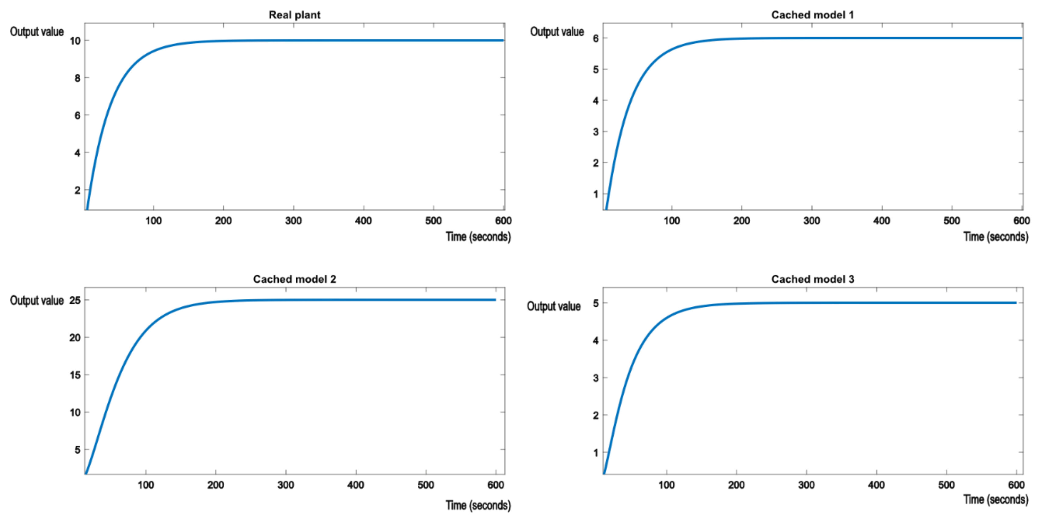
The system reference will be set to 10. It is expected that when the switch occurs from one model to another, after a brief hysteresis period, the proper nominal model, which best matches the real plant from Equations (23)–(25), will have its output stabilized around the reference value of 10. Figure 6 shows the initial evolution of the real plant and nominal models. Real plant tracks the reference value of 10 without any errors.

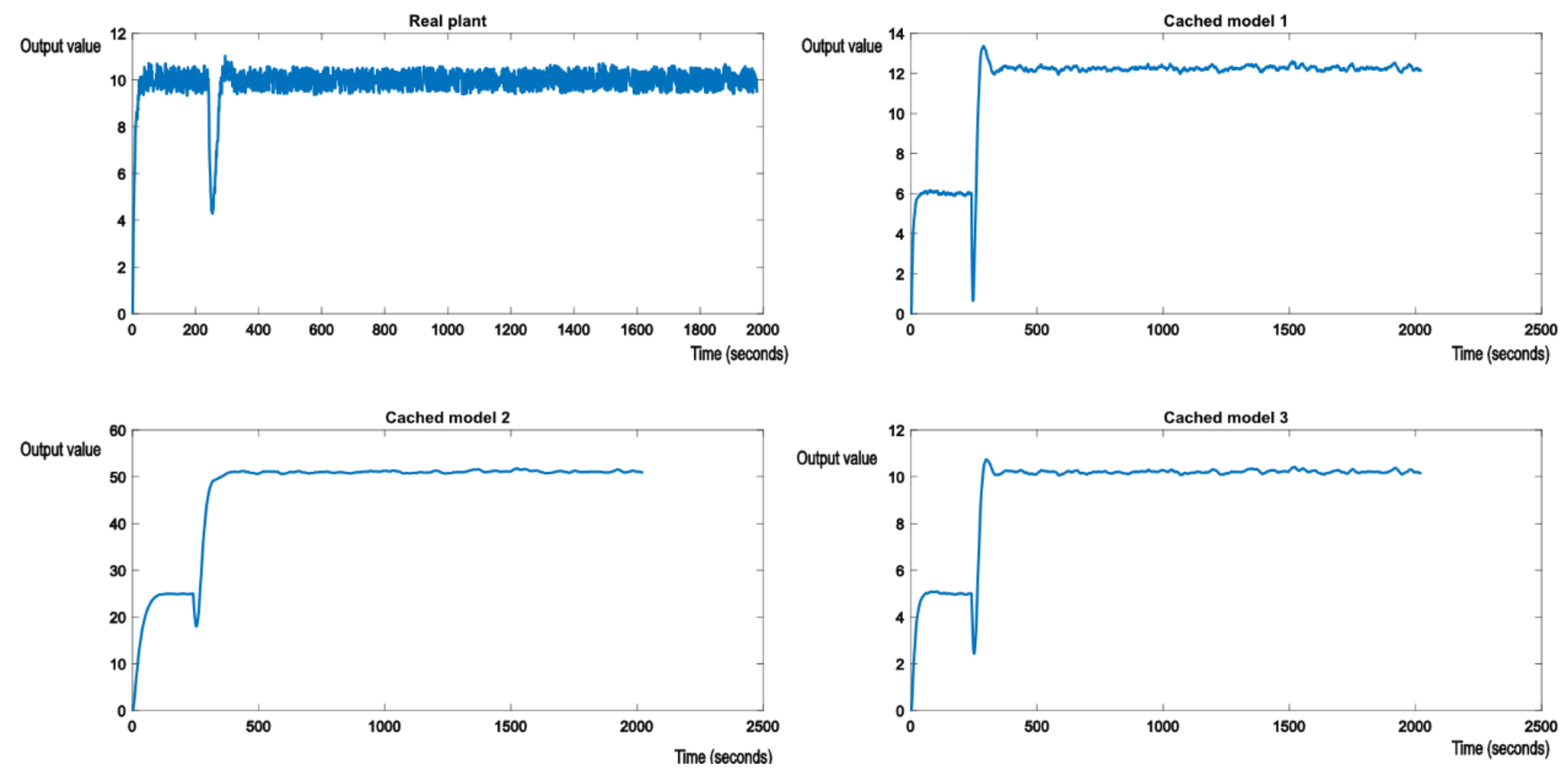
The real plan is then exposed to parametric perturbations, switching the real plant model to something like the model described in (24). For example, if our real plant would be the suspension system in a car, a sudden perturbation would be caused by degrading weather conditions. The supervisor will detect the degradation in performance and will proceed to look for a model in the knowledge base that will offer better performance. The evolution is shown in Figure 7.

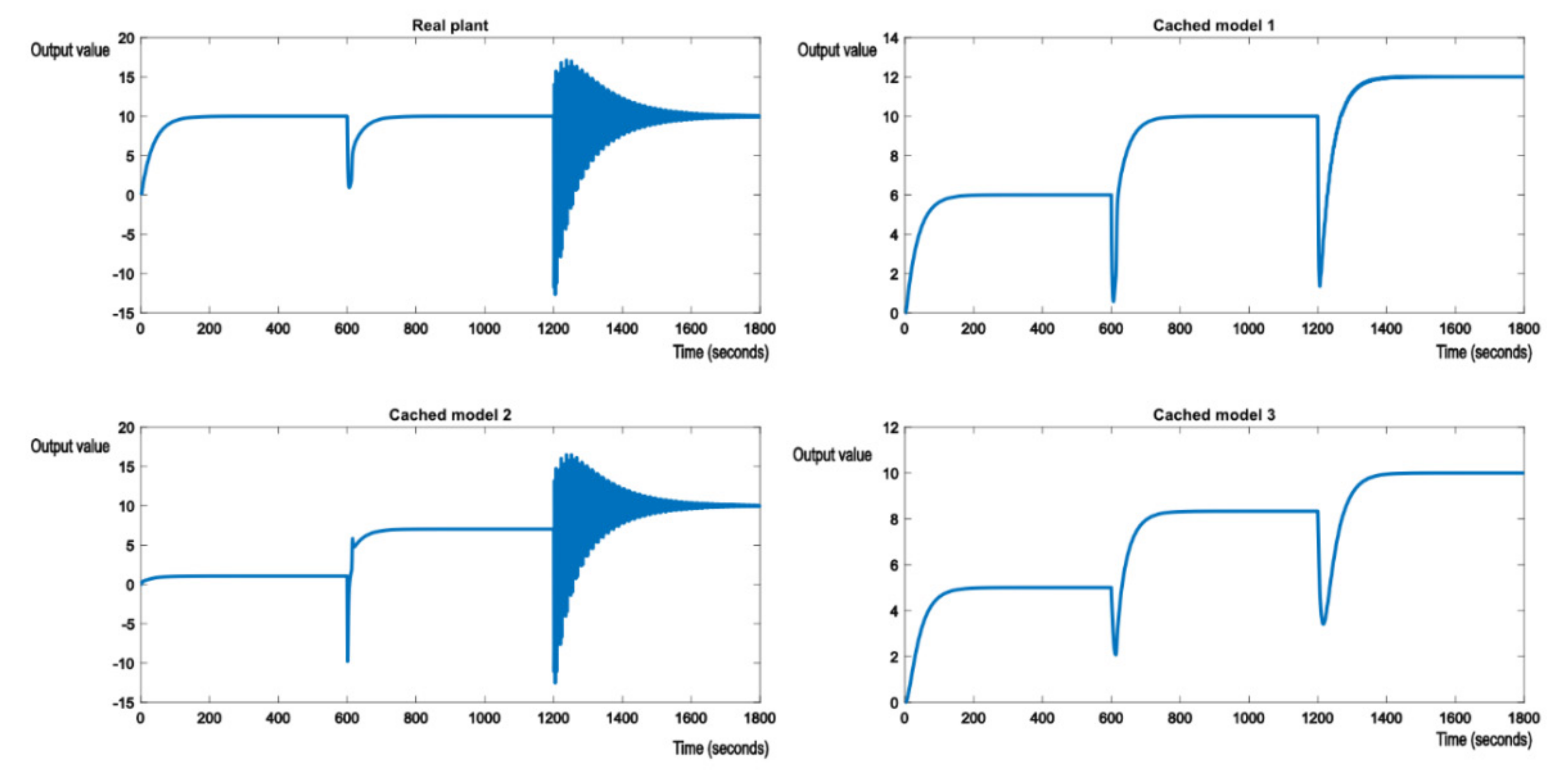
Figure 7 shows that the switching logic is working as expected and allows the system to maintain the required performance. It can also be seen that the shock of the perturbation is forwarded to the nominal models in the cache, as the output errors of the real system are passed as parameters to the GPU shader. As expected, cached model 3, which matches the transfer function (25), stabilizes at the reference value, along with the real plant. At this point, the optimal controller of (25) is also applied to the real plant, to achieve best possible performance. This is felt in the evolution of the other two cached models, which change their output values to 12 and 50. 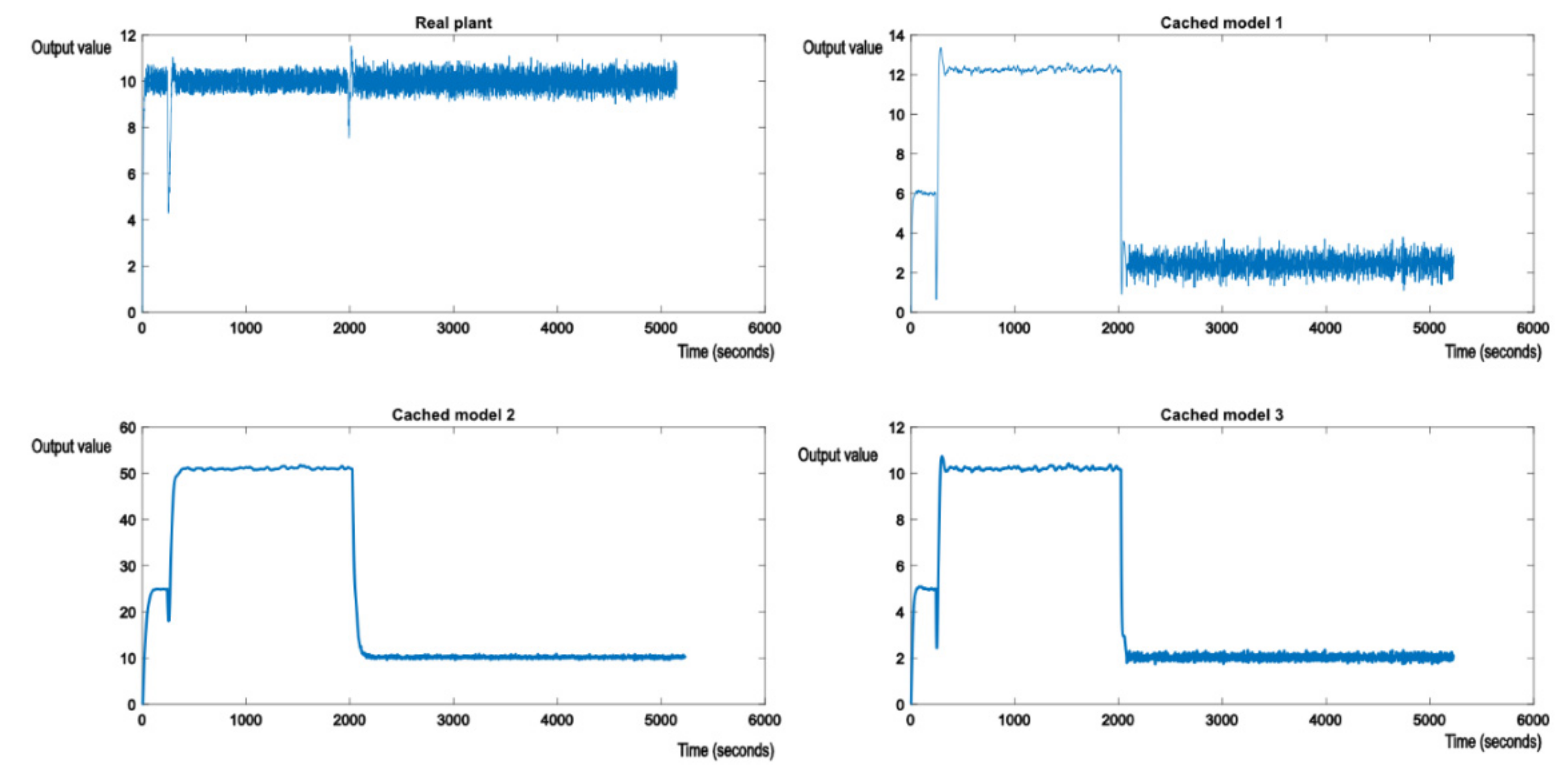Figure 8 shows another switch in the perturbation, this time to something like the nominal model (24). The behavior is very much the same. Cached model 2, which matches model (24), stabilizes to the reference value of 10, along with the real plant.

Cached model 3, no longer offering best performance, degrades along with cached model 1 to output value 2. Similar behavior will be observed with a switch to model (24). If the output value measurement is polluted by a white noise, it can be removed through filtering. In the following examples, a moving average filter with window size 4 was applied to even out the measurement noise. This means the values of CM and CP from (1) will be applied on mean of the last four output values read. Figure 9 shows the effect of perturbations applied to the real plant by altering its model to match (25). This is the same case as shown in Figure 7, but with white noise affecting the measurement of the system output.

As expected, nominal model 3 from the cache will now have its value gravitating around the reference value, but not quite matching it, due to the white noise polluting the output measurements of the real plant (but at a much lower intensity). The analogue of Figure 8 with measurement noise is shown in Figure 10.

Simulating structural perturbances is achieved by having some second order systems in the nominal model knowledge base. To keep the same low number of models, the second model, cached model 2, will be replaced with various second order transfer functions.

$${\mathrm{M}}_2 = \frac{1}{{\mathrm{s}}^2+2\mathrm{s}+1}$$

(26)

Similar tests have been conducted to demonstrate the behavior of the control system. Figure 11 shows the switch from the initial nominal model to cached model 1 (a parametric disturbance) to cached model 2 (a structural disturbance). The control scheme behaves as expected. First, nominal model 1 tracks the reference value, then when the structural perturbation occurs, the appropriate cached model 2 tracks the reference, signaling which model and controller was chosen by the control structure. In this case, the second order system behaves similarly to a first order system, because its poles lay on the real axis and have no imaginary components.

However, the closer the poles get to the imaginary axis, the more unstable the system becomes when doing the switch. For the following nominal model, shown in (27)

$${\mathrm{M}}_2 = \frac{5}{{\mathrm{s}}^2+0.1\mathrm{s}+5}$$

(27)

The system will show oscillations when switching, as shown in Figure 12. This occurs because the poles of (27), $-0.1 \pm 2\mathrm{i}\sqrt{5}$, are close to the imaginary axis, and this is known to make the system unstable, on top of the systemic shock caused by switching and disturbances. This leads to strong oscillations the moment the perturbation occurs and eventually oscillations around the reference value. Unlike oscillations caused by noisy measurements, these cannot be trivially removed using simple filters.

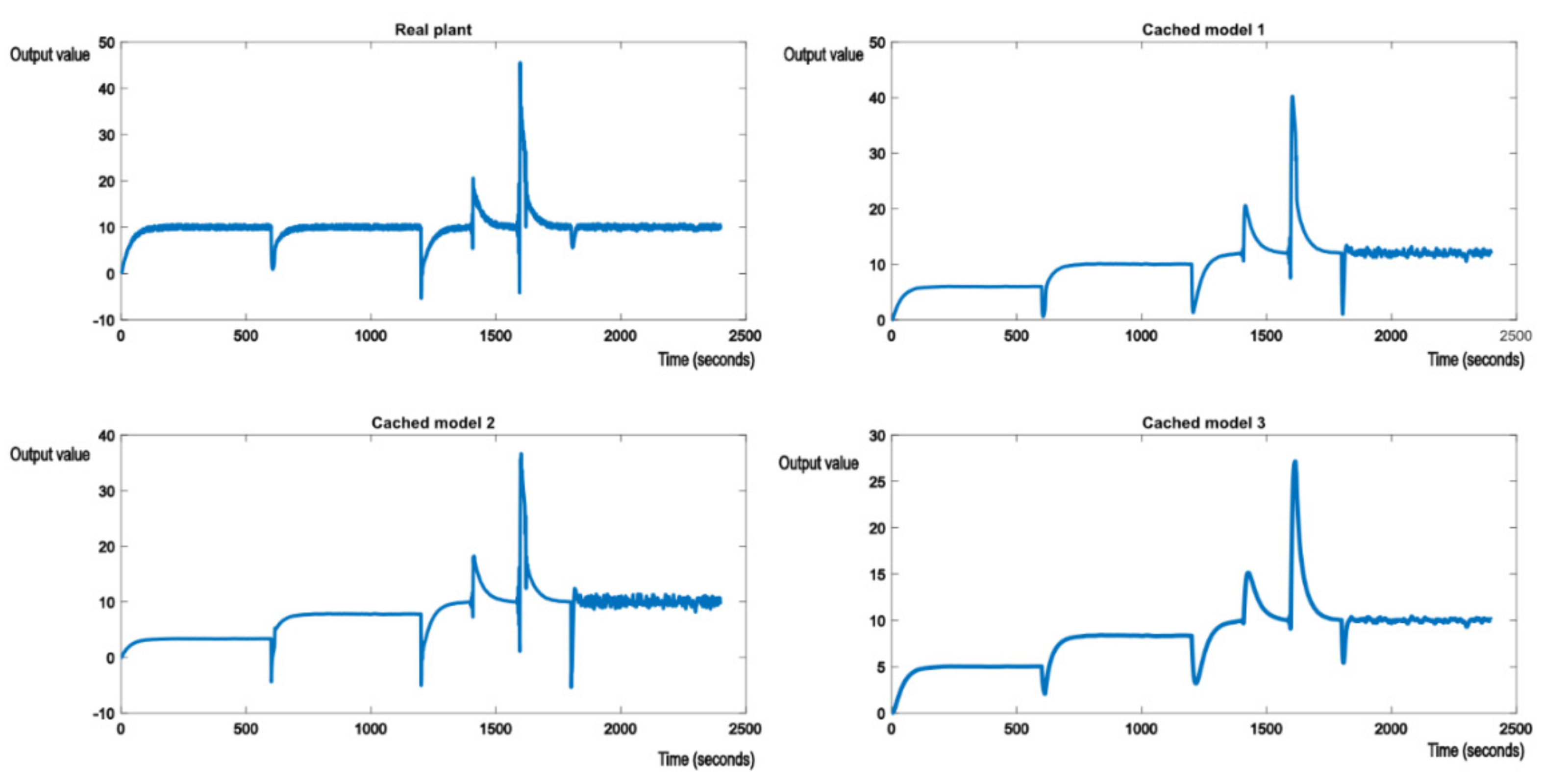
When dealing with noisy measurements of the output error, the MA filter is still good in case of structural perturbances, as shown in Figure 13. Additionally, Figure 13 shows a series of switches between various types of models, Equations (23), (25) and (26).

As far as performance is concerned, GPUs are designed to deal with large data sets. Depending on the technical specifications, a GPU can handle thousands of parallel computations of the switching criterion without performance degradations. This allows the control system to provide real time responses even for real plants that work in extremely varied working conditions.

Table 1. Performance figures for compute shaders with various number of elements. Performance is subject to variations based on hardware specifications, its power state, operating system, and driver version. All values are averages over 600 samples. Memory copy from GPU to CPU also involves converting raw bytes to the data structures describing model state, which is why it is slightly slower and consumes the better part of the GPU operation.

No. of Models	Input Buffer Create	Compute Dispatch	Memory Copy from GPU to CPU
100	~0.0202 ms	~0.3998 ms	~1.2346 ms
1000	~0.0365 ms	~0.5479 ms	~2.8668 ms
10,000	~0.1506 ms	~1.3838 ms	~18.5257 ms

shows the time taken to finish the shader invocation with an increasing number of nominal models in the knowledge base. Using GPUs is therefore best in situations where the potential number of nominal models is high. Because performance is strictly tied to hardware, we can observe that execution times do not have a linear increase. For 100 and 1000 models, the execution time does not grow in a linear fashion, with only a slightly 2× increase in execution time for a 10× increase in the number of models. Things take a turn for the worse at 10,000 models copying of structured data from GPU memory to CPU memory.

4. Discussion

The premises of the research were to show that GPUs and compute shaders can be used in real time systems control. The adaptive robust multimodel control philosophy is a perfect place to apply such technologies, as the parallel nature of the GPU hardware makes it extremely easy to handle many nominal models in the knowledge base, perhaps hundreds or even thousands of nominal models, and compute the value of the switching criterion for each of them in a single shader invocation. As seen in the results section, this approach works for both parametric and structural perturbations.

It was possible to use a single shader implementation for both first and second order transfer functions. Second order transfer functions can be combined to achieve higher order functions, but it may no longer be possible to use the same shader declaration for higher order functions.

Unlike traditional programming, shaders are supposed to be simple and not contain much branching logic or iterative functions. Branching logic is supported through various instructions such as if, for, and while, but it is notoriously expensive, and many have unforeseen side effects. The recommendation is to not use branching logic unless it is unavoidable. Iterative functions are usually replaced by the parallel nature of the GPU. Implementing a universal solution for all possible kinds of models is therefore possible but remains as a future research topic on the matter.

The choice of models that form the knowledge base also has a significant impact on the behavior of this control scheme. As physical processes can be represented by several transfer functions, it is possible that the chosen model from the knowledge base will not always be the expected one. If its robust controller provides decent performance, then it will be deemed good enough by the supervisor. This is because the robustness margin from (1) creates a zone of stability around nominal models, and any other model that fits in that zone will be a good match for the robust controller (although maybe not optimal). This can be adjusted by using a different criterion for detecting performance degradation.

Another important aspect regarding the choice of models is stability. The results show that poorly dumped or undumped models will introduce instability, and this instability is further augmented by the shock of switching. This control scheme is therefore not suitable for handling such models, but this is not related to the use of GPUs.

Output measurement noise was filtered out using a moving average filter. This worked very well, as seen in the results section, but it may not always be the best choice. Assuming more information is known about the system and the type of disturbances it may encounter, other time domain filters like band pass biquad filters or other time domain IIR filters may be used for removing the noise.

The potential applicability of compute shaders in real time control is extensive. Most modern vehicles now come equipped with GPU hardware, as infotainment systems or state of the art car status systems no longer use mechanical knobs or gauges but use high resolution displays and touchscreens to show information to drivers, sometimes even in 3D. This requires powerful GPU hardware that can keep up with real time considerations. The GPUs can potentially be used to keep track of the many electronic control units in modern cars and act as powerful supervisors over the good functioning of cars. Future research will explore the usability of compute shaders in fault detection and recovery.

As performance scales very well with a large number of models in the knowledge base, the GPU approach makes it possible to use multimodel control with a large knowledge base for fast systems, where the sampling period imposes a hard limit on the number of models, as traditional CPUs will have limited scalability due to a lower number of cores.

5. Conclusions

This article presented the use of graphics processing units in real time adaptive robust multimodel control, which is best suited for processes that may encounter repetitive types of parametric or structural perturbances. The multimodel aspect of this implementation is based on a knowledge base of previously discovered nominal models and their robust controllers. Graphics processing units are designed to deal with massive parallel computations and are extremely proficient at dealing with large knowledge bases, containing hundreds or thousands of models matching various types of perturbances that the real process may encounter during its function. The knowledge base can be filled in advance, depending on the knowledge on the functional environment of the plant, or it can be combined with an adaptive closed loop identification algorithm that discovers new working models for the plant and fills in the knowledge base in real time.

The results section showed how the control scheme would behave when dealing with parametric and structural perturbances, both with and without output measurement noise. The algorithms performed as expected, showing that graphics processing units and compute shaders can be used in real time control.

Future research will focus on implementing the control model on physical systems and implementing more of the adaptive-robust control scheme using the GPU. This includes implementing the PID tuning algorithms and system identification procedures on the GPU, thus removing the dependency on third party software, such as MATLAB.

References

1. Popescu, D.; Gharbi, A.; Stefanoiu, D.; Borne, P. Process Control Design for Industrial Applications; John Wiley & Sons: Hoboken, NJ, USA, 2017. [Google Scholar]
2. Afshar, S.; Paunonen, L. Adaptive robust output regulation control design. In Proceedings of the 2019 American Control Conference (ACC), Philadelphia, PA, USA, 10–12 July 2019. [Google Scholar]
3. Liu, K.Z.; Yao, Y. Robust Control: Theory and Applications; John Wiley & Sons: Hoboken, NJ, USA, 2016. [Google Scholar]
4. Lupu, C.; Borne, P.; Popescu, D. Multi-model adaptive control for nonlinear system. J. Control Eng. Appl. Inform. 2007, 40, 108–112. [Google Scholar] [CrossRef]
5. Narendra, K.S.; Driollet, O.A.; Feiler, M.; George, K. Adaptive control using multiple models, switching, and tuning. Int. J. Adapt. Control Signal Process. 2003, 17, 87–102. [Google Scholar] [CrossRef]
6. Lupu, C.; Mihai, C.C.; Secuianu, F.D.; Petrescu, C. Fast Disturbance Rejection in MIMO Process Based on Algorithms Switching. In Proceedings of the 2018 22nd International Conference on System Theory, Control and Computing (ICSTCC), Sinaia, Romania, 10–12 October 2018. [Google Scholar]
7. Li, W.; Ke, H. Adaptive control using multiple models without switching. J. Theor. Appl. Inf. Technol. 2013, 53, 229–235. [Google Scholar]
8. Mihai, C.C.; Lupu, C.; Secuianu, D.; Vulpe, A. Implementing high performance system simulators using modern graphics rendering devices: Implementing system control algorithms on graphics hardware. In Proceedings of the 14th International Conference on Engineering of Modern Electric Systems (EMES), Oradea, Romania, 1–2 June 2017. [Google Scholar]
9. Narendra, K.S.; Han, Z. Adaptive Control Using Collective Information Obtained from Multiple Model. IFAC Proc. Vol. 2011, 44, 362–367. [Google Scholar] [CrossRef] [Green Version]
10. Narendra, K.S.; Balakrishnan, J. Adaptive Control Using Multiple Models. IEEE Trans. Autom. Control 1997, 42, 171–187. [Google Scholar] [CrossRef]
11. Khronos Group. Rendering Pipeline Overview. Available online: https://www.khronos.org/opengl/wiki/Rendering_Pipeline_Overview (accessed on 15 July 2021).
12. Khronos Group. Compute Shader. 2019. Available online: www.khronos.org/opengl/wiki/Compute_Shader (accessed on 16 July 2021).
13. nVidia. Nvidia Turing Gpu Architecture Whitepaper. 2019. Available online: https://images.nvidia.com/aem-dam/en-zz/Solutions/design-visualization/technologies/turing-architecture/NVIDIA-Turing-Architecture-Whitepaper.pdf (accessed on 15 May 2021).
14. Microsoft Corporation. Compute Shader Overview. 31 May 2018. Available online: https://docs.microsoft.com/en-us/windows/win32/direct3d11/direct3d-11-advanced-stages-compute-shader (accessed on 15 July 2021).
15. Microsoft Corporation. Pipeline Stages (Direct3D 10). 31 May 2018. Available online: https://docs.microsoft.com/en-us/windows/win32/direct3d10/d3d10-graphics-programming-guide-pipeline-stages (accessed on 15 July 2021).
16. Microsoft Corporation. Accessing Resources. Available online: https://docs.microsoft.com/en-us/windows/win32/direct3d11/direct3d-11-advanced-stages-cs-access (accessed on 17 July 2021).
17. Mihai, C.C.; Lupu, C.; Vulpe, A.A. Using graphics processing units and openGL in adaptive-robust real time control. In Proceedings of the 2020 12th International Conference on Electronics, Computers and Artificial Intelligence (ECAI), Bucharest, Romania, 25–27 June 2020. [Google Scholar]
18. MathWorks. PID Tuning Algorithm for Linear Plant Model. Available online: https://www.mathworks.com/help/control/ref/lti.pidtune.html (accessed on 10 August 2021).
19. MathWorks. Calling MATLAB as COM Automation Server. Available online: https://www.mathworks.com/help/matlab/call-matlab-com-automation-server.html (accessed on 10 August 2021).
20. Microsoft Corporation. Visual Studio Community. Available online: https://visualstudio.microsoft.com/vs/community/ (accessed on 3 February 2021).
21. Gliga, L.I.; Mihai, C.C.; Lupu, C.; Popescu, D. Adaptive—Robust control a computational efficient real time simulation. In Proceedings of the 2015 13th International Conference on Engineering of Modern Electric Systems (EMES), Oradea, Romania, 11–12 June 2015. [Google Scholar]
22. Khronos Group. Shader Compilation. Available online: www.khronos.org/opengl/wiki/Shader_Compilation (accessed on 16 July 2021).
23. Lupu, C.; Petrescu, C.; Popescu, D. Practical Solution for Software Implementation of Algorithms Switching in Multiple Models Control Systems. In Proceedings of the CSCS15—Control Systems and Computer Science, Bucharest, 25–27 May 2005. [Google Scholar]
Figure 1. Example of working regimes a plane may encounter during its trip. Depending on weather conditions and drive path, several different controllers might be needed for its direction system.
Electronics 10 02462 g001
Figure 2. Overview of multimodel control scheme. The blue blocks on the left represents the algorithm selector block; the yellow and green blocks on the top right represents the model selection block. A model is chosen using inputs from the real process. Based on the chosen model, a control algorithm is chosen to issue new commands to the process.
Electronics 10 02462 g002
Figure 3. Detailed view of a work group of an nVidia Turing GPU. The group consists of arithmetic cores split into two subgroups and several support units that perform advanced mathematical operations (such as trigonometric operations) [13].
Electronics 10 02462 g003
Figure 4. Overview of a compute shader dispatch. The top figure shows the layout of working groups with a glDispachCompute(4, 3, 2) invocation. There are 24 total work groups. The bottom figure shows the zoomed in layout of a work group, with local_size_x = 3, local_size_y = 2, local_size_z = 2. Each work group therefore contains 12 threads. The glDispatchCompute invocation resulted in a total of 288 threads running in parallel.
Electronics 10 02462 g004
Figure 5. Overview of the work group layout of the compute shader used to calculate the switching criterion, with local_size_x = 1024, local_size_y = local_size_z = 1. Each box represents an instance of the data structure associated with a nominal model used to pass information to and from the GPU.
Electronics 10 02462 g005
Figure 6. Initial evolution of the real process and the nominal models in the knowledge base.
Electronics 10 02462 g006
Figure 7. Evolution of the real plant and the nominal models after exposing the real plant to perturbations.
Electronics 10 02462 g007
Figure 8. Evolution of the real plant and the nominal models after exposing the real plant to perturbations, switching from model 3 to model 2.
Electronics 10 02462 g008
Figure 9. Evolution of the real plant and the nominal models after exposing the real plant to perturbations, with output measurement noise.
Electronics 10 02462 g009
Figure 10. Evolution of the real plant and the nominal models after exposing the real plant to perturbations, switching from model 3 to model 2, with measurement noise.
Electronics 10 02462 g010
Figure 11. Switching from the initial model to cached model 1 and then to cached model 2.
Electronics 10 02462 g011
Figure 12. Switching from the initial model to cached model 1 and then to cached model 2, a poorly dumped second order transfer function.
Electronics 10 02462 g012
Figure 13. A series of switches between various models, mixed structural and parametric perturbances with noisy output measurements.
Electronics 10 02462 g013