NDF of Scattered Fields for Strip Geometries

Abstract

Solving inverse scattering problems by numerical methods requires investigating the number of independent pieces of information that can be reconstructed stably. To this end, we address the evaluation of the Number of Degrees of Freedom (NDF) of far-zone scattered fields for some strip geometries under the first-order Born approximation. The analysis is performed by employing the Singular Value Decomposition (SVD) of the scattering operator in the two-dimensional scalar geometry of one or more strips illuminated by a TM polarized plane wave. It is known that investigating the scattering scene at different incident plane waves (multi-view configuration) enhances the NDF. Therefore we mean to examine the minimum number of incident plane waves providing the NDF of the scattered fields both by theoretical estimations and numerical verifications.

1. Introduction

The electromagnetic scattering problem deals with determining the scattered field produced by a specified scatterer when incident plane waves illuminate it. This defines the so-called direct or forward problem. The inverse scattering problem aims at determining the features of an unknown scatterer, like its material, configuration (shape), and position, from information about its scattered fields under known excitation fields. The electromagnetic waves can be applied to investigate hidden or remote regions. The imaging algorithms based on inverse scattering methods are appropriate for a broad range of applications, such as medical imaging and subsurface imaging [1,2], ground-penetrating radar (GPR) [3,4,5,6], radar imaging, and military applications [7,8].

Under some circumstances, the imaging equation can be cast as a linear operator between the scattering object and the related far-zone scattered fields. In this case, the Singular Value Decomposition (SVD) provides a very powerful mathematical tool to investigate the ultimate capabilities of the imaging algorithms. In particular, it is important to examine the maximum amount of information that can be retrieved from the data in the presence of noise [9], so as to obtain an imaging algorithm providing results that are not affected by the unavoidable uncertainties on data.

The Number of Degrees of Freedom (NDF) of the scattering object can be identified as this number of meaningful data and corresponds to the principal (i.e., above a fixed threshold) singular values of the relevant operator. If the operator is compact, its singular values cluster to zero [9] so that the NDF is always limited and commonly noise-dependent [10]. When the singular values exhibit a steplike behavior, the NDF can be regarded as near noise independent only for a minimal number of instances [11,12].

The NDF has been studied for a few decades for optical imaging applications [13,14,15]. In imaging and, generally, in inverse problems, the NDF measures the rank deficiency of the forward operator and hence the ill-posedness of the problem [16]. A method for determining NDF in inverse scattering under Born approximation has been proposed in [17].

In References [18,19,20], a different problem is considered, i.e., the inverse source problem when a (2D) source current must be reconstructed from its radiated field. Our investigation focused on estimating the NDF of the source according to its geometry so that a robust imaging algorithm can be set up. This can be achieved by the SVD of the relevant radiation operator, analytically, when possible, by asymptotic upper bounds or numerically. For instance, circumference [18], angle [19], and conic [20] sources have been examined. In particular, in [19], theoretical arguments are developed for a collection of linear sources to show the role of their total electrical length to determine their NDF.

In this paper, we deal with the inverse scattering problem, which is the reconstruction of an object from the fields scattered by it under different plane wave excitations. Within the Born approximation, again, a linear operator that connects the object to the fields is obtained, and, again, the question of the NDF of the whole set of scattered fields can be investigated. It is, now, a different operator, since the scattered depends on two angle variables, i.e., the observation angle and the direction of the impinging plane wave. Since the problem is new and the results depend on the object geometry, in order to appreciate the main factors affecting it, we start considering some simpler geometries, in particular, when the whole investigation domain is composed of a collection of linear domains. Thus, following the same approach of [19], it is possible to establish a connection between the NDF and their total electrical length.

Therefore, the principal purpose of this paper is to examine the NDF of the scattered fields of strip geometries and, in addition, to investigate the number of independent plane wave excitations. It can be mentioned that finding the minimum number of independent plane waves and observation points are related to the NDF. In [21], the same problem of investigating the NDF of the fields scattered by an object under the Born approximation is considered. However, a different 2D geometry is taken into account, i.e., a circle, and a very large upper bound on the NDF is established first, founding on reciprocity arguments. A numerical study is then performed for objects varying either only along the radial coordinate or only along the azimuthal coordinate. The main goal of the paper was to establish that only a limited set of object functions can be reconstructed within the Born approximation, requiring not only low-contrast value functions, but also slow spatial variations.

The second goal is to compare the performances of the operators resulting from the use of different variables within the scattering operator definition. Finally, we present numerical reconstructions for each geometry to confirm the results.

The paper is organized as follows. Section 2 introduces the formulation of the problem and the main definitions that are used in the following sections. In Section 3, we recall the previous results about the one strip geometry and present new results. Next, we consider the cases of the two strips (Section 4) and the cross-strip (Section 5) geometries, respectively. Finally, we summarize and discuss the results in Section 6.

2. Problem Statement

This section aims at providing some mathematical preliminaries and notations used in the following sections. In general, the scatterer can be either dielectric or perfect electrically conducting (PEC); here, we consider the dielectric case, where the Born approximation leads to a linear scattering operator. For PEC objects, the Physical Optics approximation can be invoked for electrically large convex objects. Again, the corresponding scattering operator is linear with the same kernel as in [1], and an unknown distributional function representing the object shape [22]. Therefore, the whole discussion can be extended promptly to the PEC case.

The geometries we intend to analyze and examine are composed of the scatterer located within a homogeneous medium with dielectric permittivity ${ϵ}_0$ and magnetic permeability ${\mu }_0$. The scatterer can be one strip, two strips, and the cross strip.

Generally, the relationship between the scattered field and the scatterer is nonlinear. This nonlinearity arises from multiple scattering effects inside the scatterer. However, a linear relationship can be found sometimes when only a single scattering event is important. Either Born or Rytov approximations can be used to calculate the scattered field, which leads to a Fourier transform relationship between the scattered field and the scatterer. Consequently, the simplest method to linearize the inverse scattering is to use the first-order Born approximation [23,24]. In the Born approximation, the total field inside the scatterer domain is approximated by the incident plane wave. This linear approximation is only valid for smaller scatterers with low contrast compared to the background medium, but also holds for metallic objects.

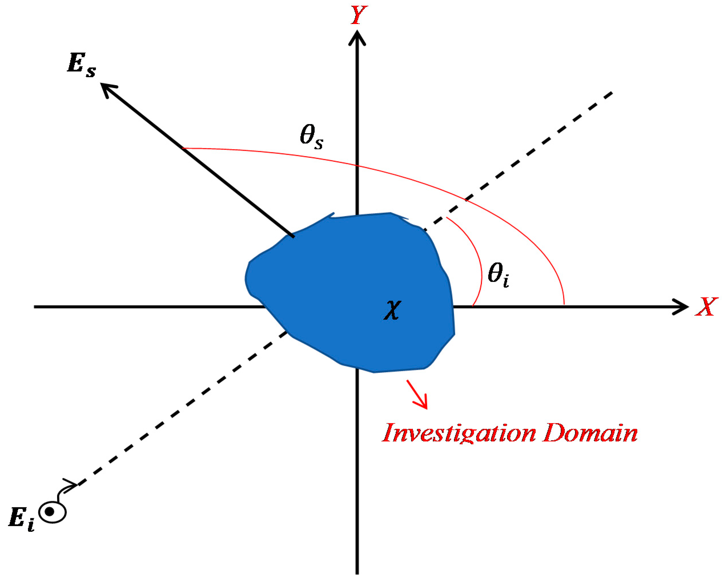
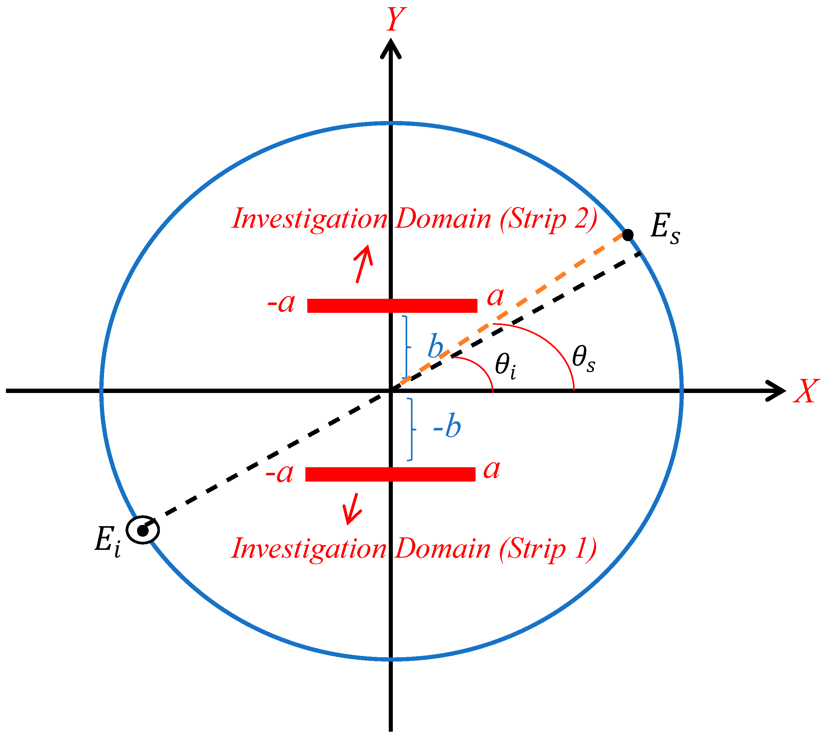
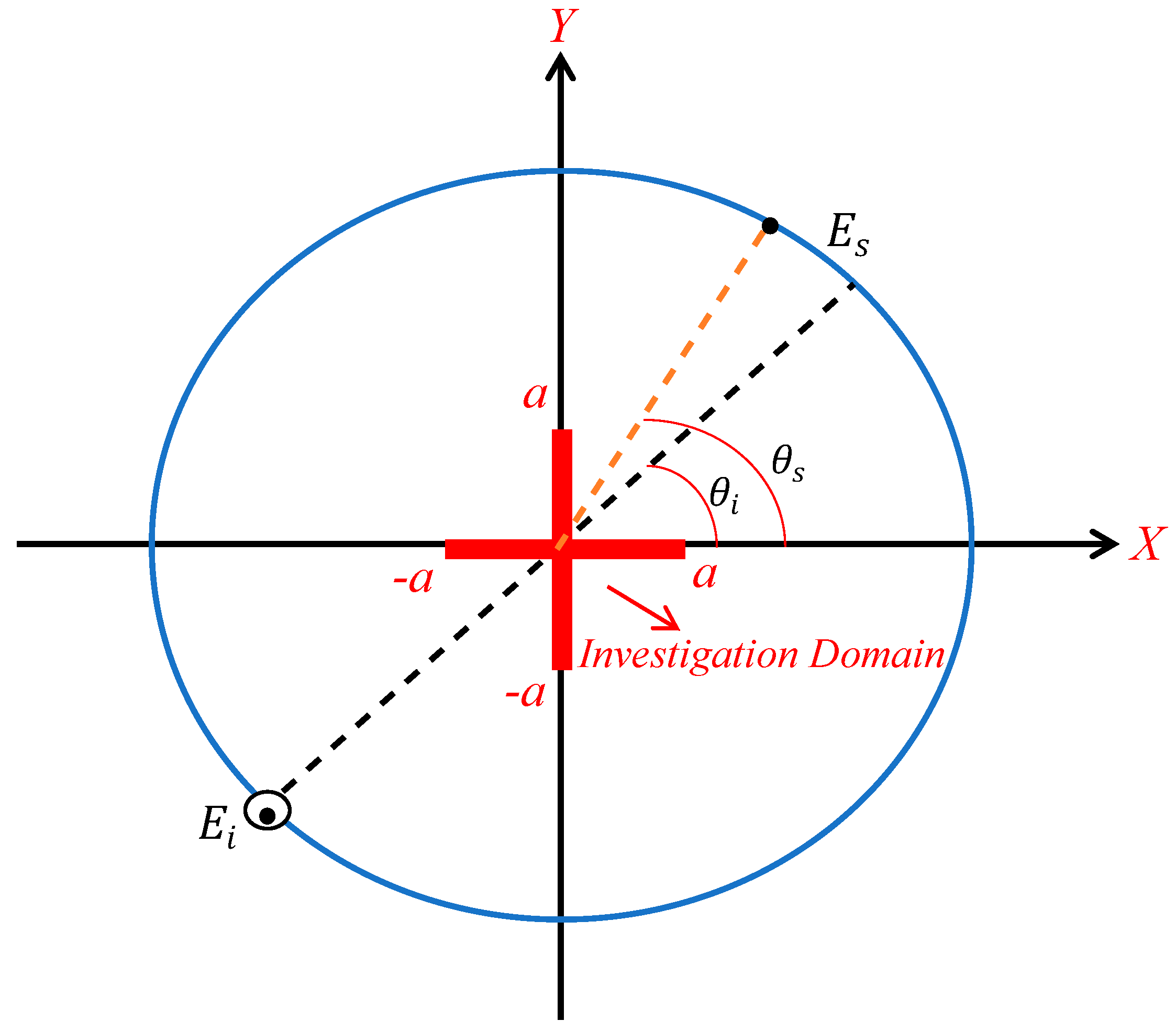
Figure 1 illustrates a general diagram of the inverse scattering problem. An unknown scatterer is located in a domain referred to as the Investigation Domain (ID), and the incident plane wave $E_i$ illuminates it; then for each angle of illumination, the scattered fields $E_s$ are measured at observation angles external to the ID in the scatterer’s far zone. We denote by ${\theta }_i$ the angle defining the direction of propagation of the incident plane wave, and by ${\theta }_s$ the observation angle of the scattered field. The scattering sensing can be probed by changing the incidence angle to improve reconstruction performance and increase the NDF (multi-view configuration).

Hence, the scattered field in the far-zone under the Born approximation for the two-dimensional scalar case can be recast as

$$E_s\left({\theta }_s\right)={\displaystyle \iint }\chi \left(x,y\right) E_i\left(x,y,{\theta }_i\right) e^{j\beta (x\cos {\theta }_s+y\sin {\theta }_s)} dxdy$$

(1)

where $\chi \left(x,y\right)$ and $E_i \left({\theta }_i\right)$ are the contrast function and the incident plane wave, respectively. An object or scatterer represented by $\chi \left(x,y\right)=1-{ϵ}_s\left(x,y\right)/{ϵ}_0$ is placed in a homogeneous background, which has a permittivity of ${ϵ}_0$, where ${ϵ}_0$ is usually the permittivity of free space. This scatterer has a relative permittivity of ${ϵ}_s\left(x,y\right)$, which is related to the scatterer. The wavenumber is denoted by $\beta =\omega \sqrt{{ϵ}_0{\mu }_0}=2\pi /\lambda$, where $\omega$ is the angular frequency, and $\lambda$ is the wavelength. The incident plane wave from the direction ${\theta }_i$ is provided by

$$E_i\left({\theta }_i\right)=e^{-j\beta (x\cos {\theta }_i+y\sin {\theta }_i)}$$

(2)

Now, the substitution of Equation (2) in (1) gives

$$E_s\left({\theta }_s,{\theta }_i\right)={\displaystyle \iint }\chi \left(x,y\right) e^{j\beta [x(\cos {\theta }_s-\cos {\theta }_i)+y\left(\sin {\theta }_s-sin{\theta }_i\right)]} dxdy={ℒ}_{\theta }\left(\chi \left(x,y\right)\right)$$

(3)

where ${ℒ}_{\theta }$ is the linear operator for the multi-view and single frequency scattering configurations of our interest. Now, since the scattering operator is linear and compact, the SVD provides a complete, powerful way to estimate the NDF as the number of significant singular values. The SVD consists of the triple $\left\{v_n, {\sigma }_n, u_n\right\}$, where $u_n$ is the 𝑛-th left singular function, ${\sigma }_n$ is the 𝑛-th singular value, and $v_n$ is the 𝑛-th right singular function [16].

Next, we can define the scattered field by using different observation variables. Let be $u_s=\cos {\theta }_s$ and $u_i=\cos {\theta }_i$. Then, $\sin {\theta }_s$ and $\sin {\theta }_i$ are achieved by

$$\sin {\theta }_s=\{ \begin{array}{c} \sqrt{1-u_s^2} 0<{\theta }_s<\pi \\ -\sqrt{1-u_s^2} 2\pi >{\theta }_s>\pi \end{array}$$

(4)

and

$$\sin {\theta }_i=\{ \begin{array}{c} \sqrt{1-u_i^2} 0<{\theta }_i<\pi \\ -\sqrt{1-u_i^2} 2\pi >{\theta }_i>\pi \end{array}$$

(5)

hence, we can rewrite Equation (3) as

$$\{\begin{array}{c}{E}_s\left(u_s,u_i\right)={\displaystyle \iint }\chi \left(x,y\right)e^{j\beta \left[x\left(u_s-u_i\right)+y\left(\sqrt{1-u_s^2}-\sqrt{1-u_i^2}\right)\right]}dxdy 0<{\theta }_s<\pi \mathrm{and} 0<{\theta }_i<\pi \\ E_s\left(u_s,u_i\right)={\displaystyle \iint }\chi \left(x,y\right)e^{j\beta \left[x\left(u_s-u_i\right)+y\left(-\sqrt{1-u_s^2}-\sqrt{1-u_i^2}\right)\right]}dxdy 2\pi >{\theta }_s>\pi \mathrm{and} 0<{\theta }_i<\pi \\ E_s\left(u_s,u_i\right)={\displaystyle \iint }\chi \left(x,y\right)e^{j\beta \left[x\left(u_s-u_i\right)+y\left(-\sqrt{1-u_s^2}-\left(-\sqrt{1-u_i^2}\right)\right)\right]}dxdy 2\pi >{\theta }_s>\pi \mathrm{and} 2\pi >{\theta }_i>\pi \\ E_s\left(u_s,u_i\right)={\displaystyle \iint }\chi \left(x,y\right)e^{j\beta \left[x\left(u_s-u_i\right)+y\left(\sqrt{1-u_s^2}-\left(-\sqrt{1-u_i^2}\right)\right)\right]}dxdy 0<{\theta }_s<\pi \mathrm{and} 2\pi >{\theta }_i>\pi \end{array}$$

(6)

thus defining the ${ℒ}_u$ operator

$$E_s\left(u_s,u_i\right)={ℒ}_u\left(\chi \left(x,y\right)\right)$$

(7)

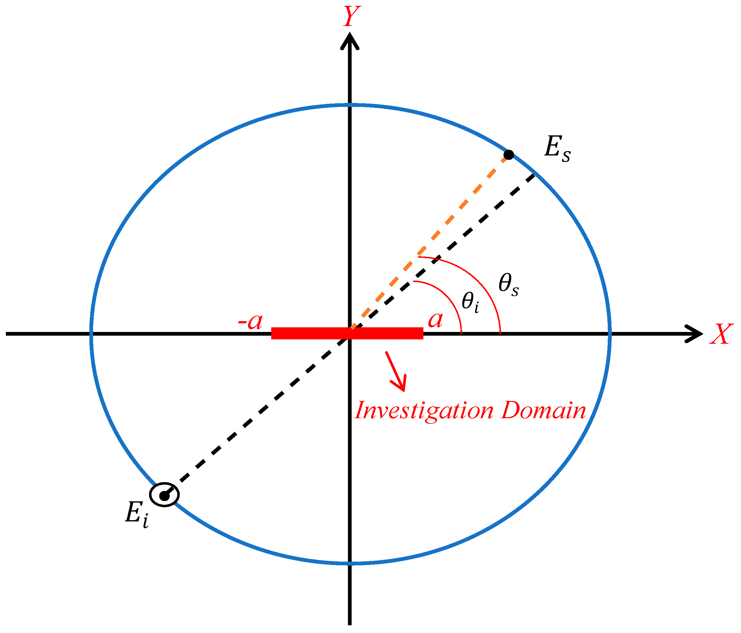
3. One strip ID Geometry

This section considers the case where the ID is one strip located on the x-axis, as shown in Figure 2, so that the ID is $I=\left[-a,a\right]$. Firstly, we analyze the problem theoretically in terms of the ${ℒ}_u$ and ${ℒ}_{\theta }$ operators to estimate the NDF, and then we simulate it numerically. We point out that the NDF of ${ℒ}_u$ can be estimated by arguments based on the Fourier Transform and sampling theory. Moreover, we intend to present a reconstruction of a smaller strip within the ID and observe the differences between the ${ℒ}_u$ and ${ℒ}_{\theta }$ operators.

The scattered far-field of one strip is derived from Equation (3):

$$E_s\left({\theta }_s,{\theta }_i\right)={{\displaystyle \int }}_{-a}^a\chi \left(x\right)e^{j\beta x(\cos {\theta }_s-\cos {\theta }_i)}dx={ℒ}_{\theta }\left(\chi \left(x\right)\right)$$

(8)

Since we consider the problem in a complex Hilbert space $\mathscr{H}$, Equation (8) defines a linear mapping:

$${ℒ}_{\theta }:\chi \in L_{\left[-a,a\right]}^2\to E_s\in L_{\left[-\pi ,\pi \right]\times \left[-\pi ,\pi \right]}^2$$

(9)

where $\chi$ and $E_s$ are supposed to belong to the set of square-integrable functions signified by $L^2 (.)$ supporting the pertinent definition domain.

In turn, the adjoint mapping of ${ℒ}_{\theta }$ is defined by

$$\langle E_s|{ℒ}_{\theta } \chi {\rangle }_{L_{\left[-\pi ,\pi \right]\times \left[-\pi ,\pi \right]}^2}=\langle {ℒ}_{\theta }^{+} E_s| \chi {\rangle }_{L_{\left[-a,a\right]}^2}$$

(10)

So that it results in

$${ℒ}_{\theta }^{+}\left(E_s\left({\theta }_s,{\theta }_i\right)\right)={{\displaystyle \iint }}_{-\pi }^{\pi } E_s\left({\theta }_s,{\theta }_i\right) e^{-j\beta x^{\prime }(\cos {\theta }_s-\cos {\theta }_i)} d{\theta }_s d{\theta }_i$$

(11)

Next, from the spectral theorem for compact self-adjoint operators applied to ${ℒ}_{\theta }^{+}{ℒ}_{\theta }$, it follows that

$$\begin{gathered} {ℒ}_{\theta }^{+}{ℒ}_{\theta }\left(\chi \right)={{\displaystyle \iint }}_{-\pi }^{\pi }{e}^{-j\beta x \prime (\cos {\theta }_s-\cos {\theta }_i)}\left[{{\displaystyle \int }}_{-a}^a\chi \left(x\right)e^{j\beta x(\cos {\theta }_s-\cos {\theta }_i)} \mathrm{dx}\right]d{\theta }_s d{\theta }_i= \\ {{\displaystyle \int }}_{-a}^a\chi \left(x\right) \left[{{\displaystyle \iint }}_{-\pi }^{\pi }{e}^{j\beta [\left(x-x^{\prime }\right)(\cos {\theta }_s-\cos {\theta }_i)]} d{\theta }_s d{\theta }_i\right] dx \end{gathered}$$

(12)

If we denote by $k\left(x-x^{\prime } \right)$ the kernel of Equation (12).

$$\begin{gathered} k\left(x-x^{\prime }\right)={{\displaystyle \iint }}_{-\pi }^{\pi }{e}^{j\beta \left(x-x^{\prime }\right)(\cos {\theta }_s-\cos {\theta }_i)}d{\theta }_s d{\theta }_i= \\ {{\displaystyle \int }}_{-\pi }^{\pi }{e}^{j\beta \left(x-x^{\prime }\right)\cos {\theta }_s} d{\theta }_s {{\displaystyle \int }}_{-\pi }^{\pi }{e}^{-j\beta \left(x-x^{\prime }\right)\cos {\theta }_i} d{\theta }_i={\left(2\pi J_0(\beta \left|x-x^{\prime }\right|\right)}^2 \end{gathered}$$

(13)

where $J_0(·)$ is the Bessel function of the first kind and zeroth order. Finally, substituting Equation (13) to (12) reads as

$${ℒ}_{\theta }^{+}{ℒ}_{\theta }\left(\chi \right)={{\displaystyle \int }}_{-a}^a\chi \left(x\right) {\left(2\pi J_0(\beta \left|x-x^{\prime }\right|\right)}^2 dx$$

(14)

Now, we define the scattered field by using the different variables, i.e., $u_s=\cos {\theta }_s$ and $u_i=\cos {\theta }_i$ [25] so that

$$E_s\left(u_s,u_i\right)={{\displaystyle \int }}_{-a}^a\chi \left(x\right) e^{j\beta (u_s-u_i)x} dx={ℒ}_u\left(\chi \left(x\right)\right)$$

(15)

Moreover, the Fourier transform operator is achieved. Its SVD is known in terms of prolate spheroidal wave functions. Moreover since $u_s,u_i\in \left[-1,1\right],$ the NDF of one strip can be estimated approximately by

$$NDF=4\left(\frac{2a}{\lambda }\right)=\frac{4\beta }{\pi /a}$$

(16)

This amount can be estimated as the number of samples of the Fourier transform of $\chi \left(x\right)$ within the full $4\beta$ spatial pulsation domain. Since this is only twice the NDF of the case of a single plane wave incidence (which can be estimated by the same arguments as above for a fixed value of ${\theta }_i$), it can be predicted that the incidence of only two plane waves can provide the NDF. In particular, the extremal values $u_i=1,-1$ allow covering of the whole Fourier domain. This means that the fields scattered by the two plane waves impinging from the ${\theta }_i=0,\pi$ incident angles may achieve all the NDF. Then, a similar result can also be expected for the ${ℒ}_{\theta },$ the operator of (8).

We present some numerical simulations in order to confirm the above discussion. They are obtained by discretizing operators (8) and (15) so that the inverse problem is equivalent to solve a system of equations whose unknowns are the discretized version of $\chi$. The frequency of the incident plane wave is 300 MHz and $\lambda =1$ m. The set of observation and incidence angles each consist of $60$ elements that are uniformly distributed in a circle in the far-zone; they are denoted by $N_{obs}$ and $N_i$.

In the numerical simulations presented here, the ID is $I=\left[-a,a\right],$ where $a$ is equal to $3\lambda$. The estimation of its NDF is $24$, by Equation (16). The choice of the dimension of the investigation domain in the test cases is not important, provided each strip is larger than the wavelength in order, the theoretical results about the NDF hold. The goal of the numerical examples is to show that a far lower number of the appropriately chosen plane is enough to achieve the NDF of the whole set of scattered fields. Consequently, increasing the number of plane waves cannot increase the NDF. For reference, we just select a sufficiently large number of plane waves, so as to be sure to achieve all the predicted NDF.

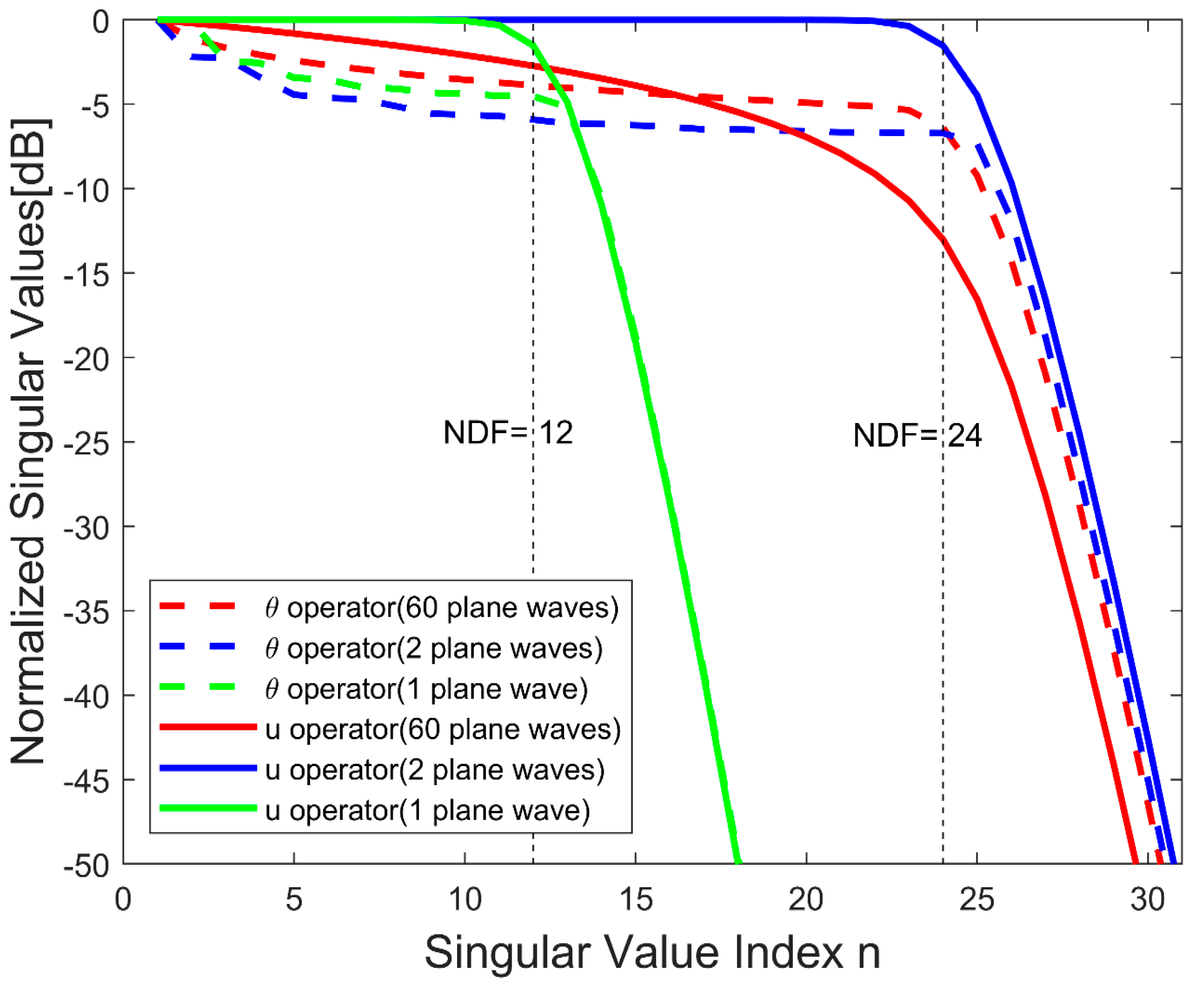
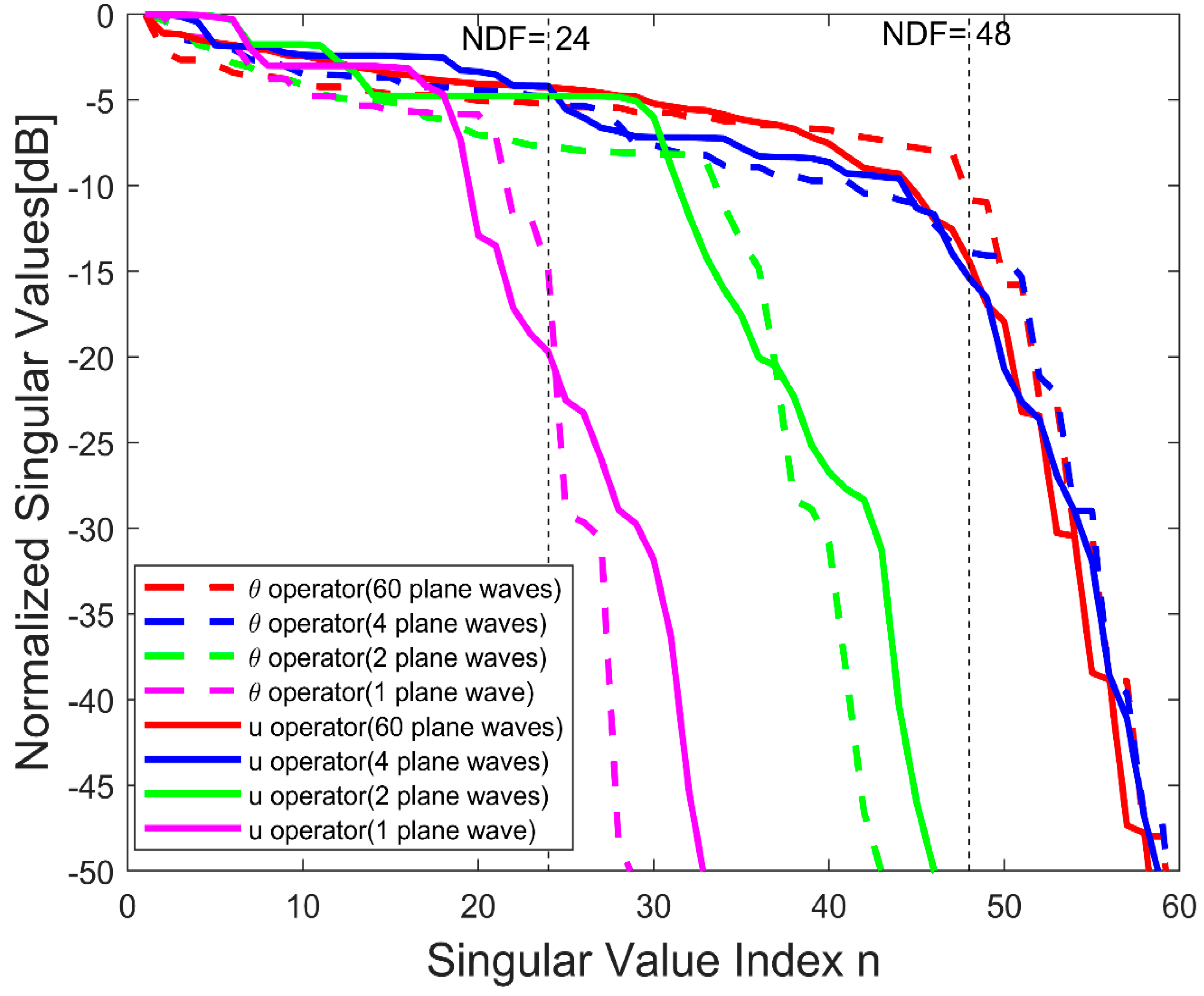
Figure 3 shows the normalized singular values of operators (8) and (15) at different numbers of incident plane waves for both ${ℒ}_{\theta }$ and ${ℒ}_u$. It can be seen that increasing the number of plane waves do not increase the NDF. For the ${ℒ}_u$ operator, the behavior of the singular values is flat, as expected from the theoretical results by the prolate spheroidal wave functions. Consequently, the only difference between the two operators is the behavior of singular values, but both operators can achieve the same NDF.

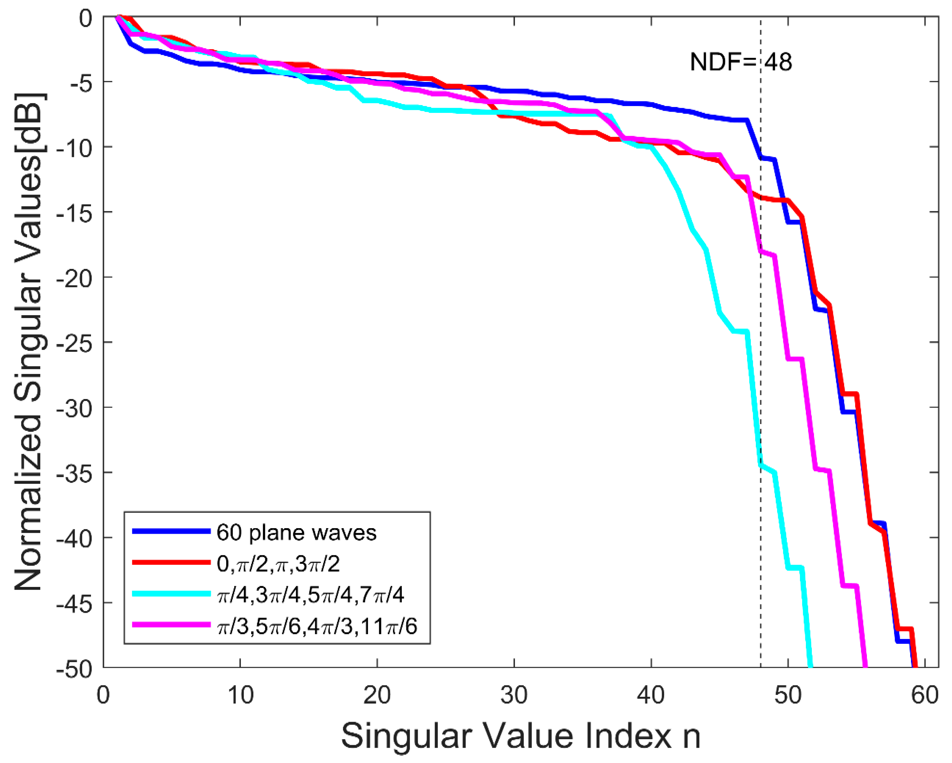
Figure 4 shows the effect of the choice of two incident plane waves from different directions on the behavior of the singular values. As can be observed, the optimal case amounts to considering the two plane waves impinging from the directions ${\theta }_i=0,\pi .$ In conclusion, the numerical results confirm that two plane waves are enough to approximately achieve the NDF.

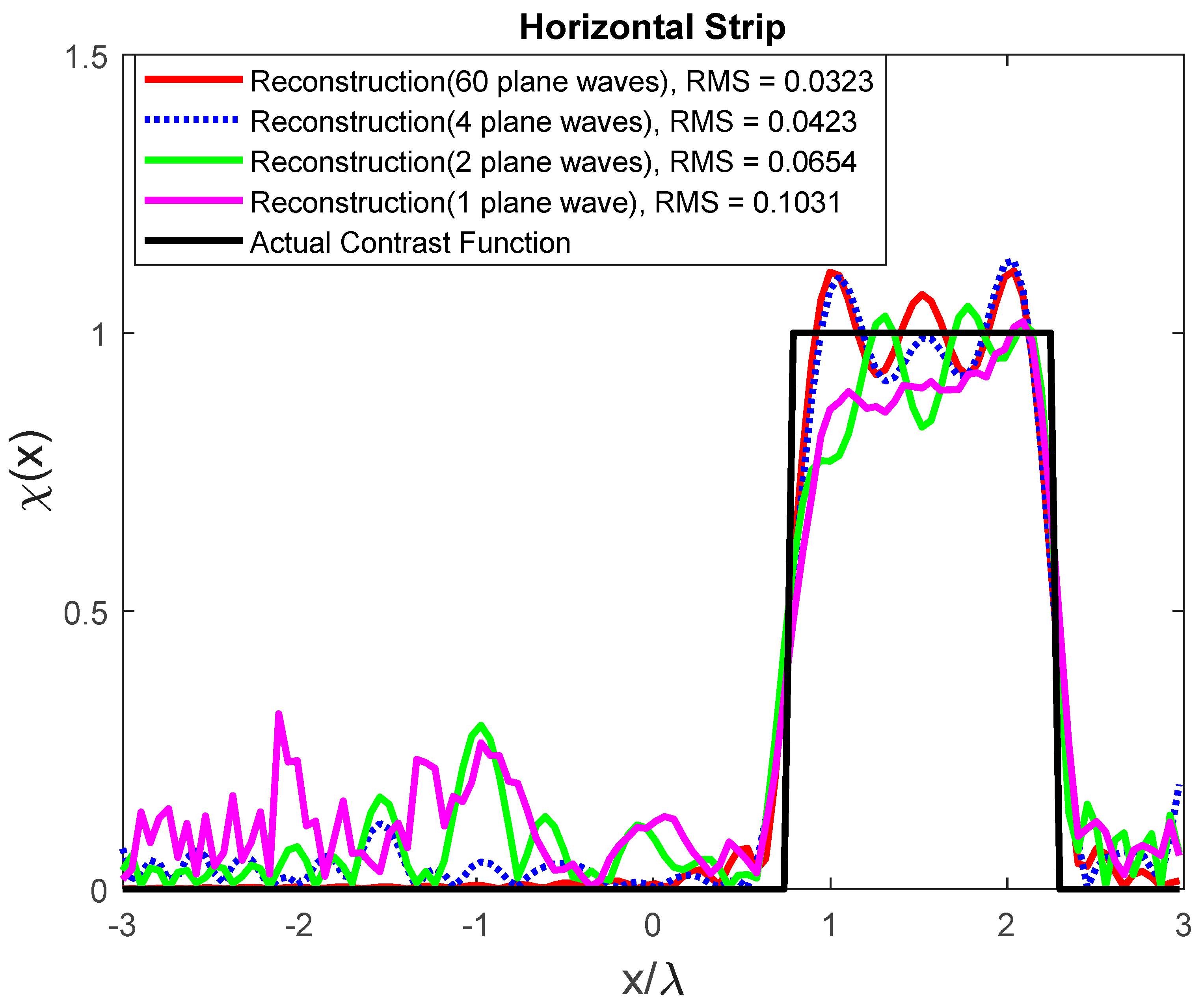
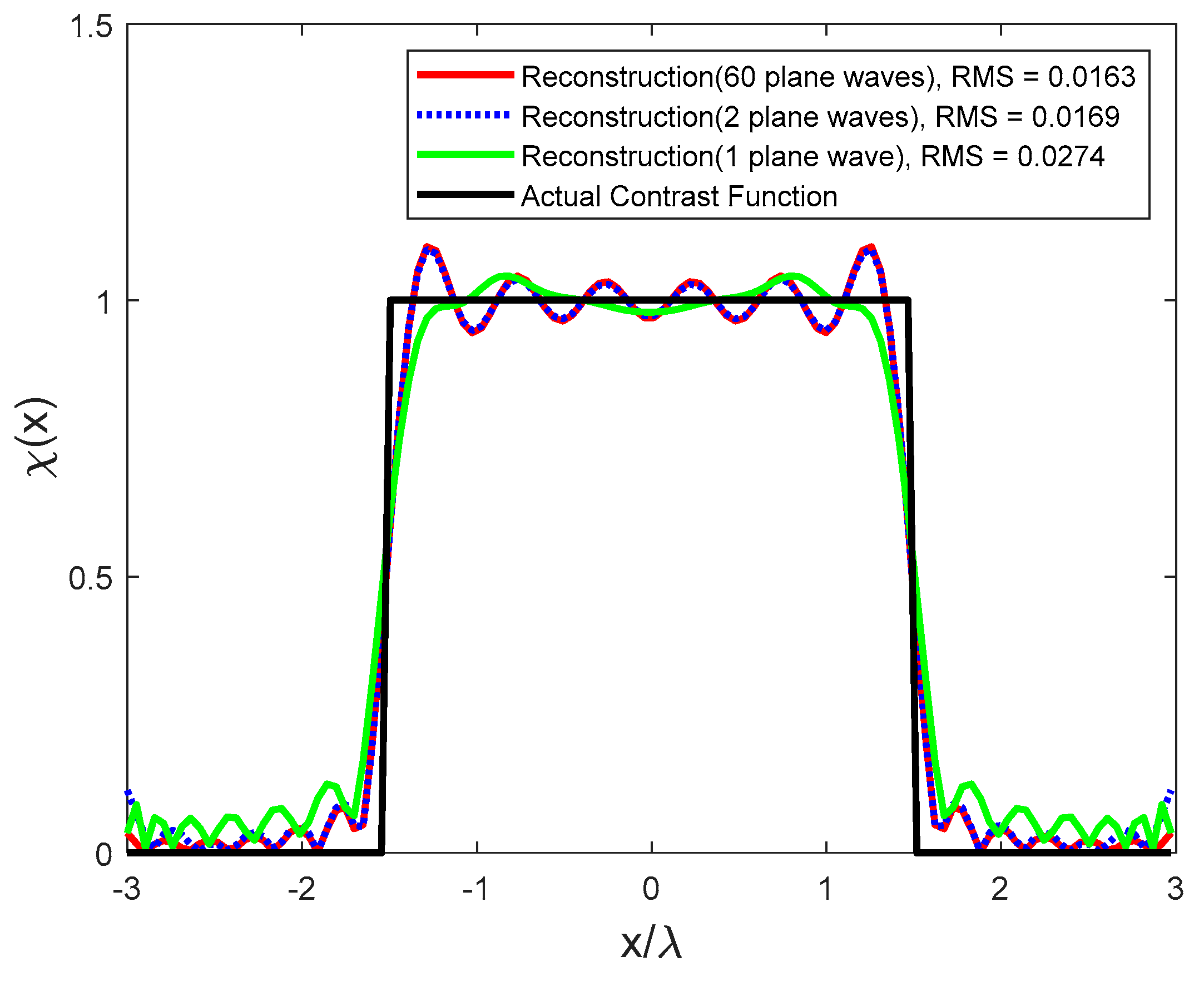
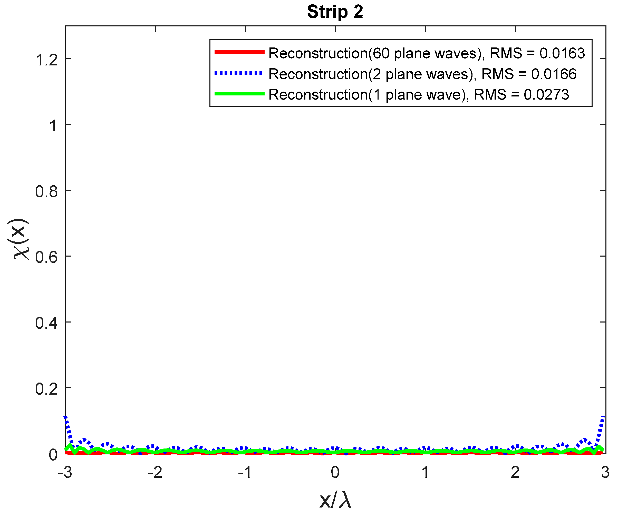
The practical relevance of discussions can be shown numerically by a reconstruction referring to a $3\lambda$ dielectric strip with $\chi =1$ as a scatterer, located within the ID. Figure 5 shows the reconstructions for different numbers of plane waves. The aim is to confirm the previous results and to show that only two plane waves are enough to achieve the best reconstructions. Scatterer reconstruction of Figure 5 confirms the expectation about the low-pass behavior of the scattering operator. As can be seen, the main lobe of reconstructions by the incidence of $60$ plane waves (red line) and two plane waves (blue dotted line) overlap.

The inversion algorithm allows us to reconstruct the object on the proper strip domain correctly, and the reconstruction accuracy for the case of two incident plane waves is the same as the case of 60 ones, while a single incidence gives a poorer result. In this way, it is confirmed that the number of independent plane waves for this ID is two.

On the other hand, the main lobe of reconstruction for one plane wave incidence (green line) is not acceptable. The Root Mean Square (RMS) can be used to compare errors of different reconstructions. As can be seen, the RMS of the two plane waves case is very close to the full case.

4. Two Strips ID Geometry

The same analysis as Section 3 is here extended to address the case of two parallel stripes along the x-axis. We consider two strips located at $I_1=\left[-a,a\right]$ and $I_2=\left[-a,a\right]$, respectively, and $d=2b$ is the distance between them so that the ID is $I_1{\displaystyle \cup }{I}_2$. The geometry of the problem is shown in Figure 6. The purpose is to find the minimum number of independent plane waves to achieve the NDF and introducing the optimal plane waves direction, which allows the achievement of all the NDF. Furthermore, we investigate the role of the distance between two strips in determining the NDF and find a rule that the whole NDF of two strips can be computed by summing the NDF of each strip. Finally, we compare the results of ${ℒ}_{\theta }$ operator with ${ℒ}_u$ operator.

The scattered far-field for strip 1 and strip 2 defines in terms of ${ℒ}_{\theta }$ operator by Equations (17) and (19), respectively.

$$\begin{gathered} E_{s1}\left({\theta }_s,{\theta }_i\right)={{\displaystyle \int }}_{-a}^a{\chi }_1\left(x_1\right) e^{j\beta x_1(\cos {\theta }_s-\cos {\theta }_i) } e^{-j\beta b(\sin {\theta }_s-\sin {\theta }_i)} d{x}_1= \\ {\mathcal{T}}_1\left({\chi }_1\left(x_1\right)\right)=e^{-j\beta b\left(\sin {\theta }_s-\sin {\theta }_i\right)} {ℒ}_1\left({\chi }_1\left(x_1\right)\right) \end{gathered}$$

(17)

where ${ℒ}_1\left({\chi }_1\left(x_1\right)\right)$ is

$${ℒ}_1\left({\chi }_1\left(x_1\right)\right)={{\displaystyle \int }}_{-\mathrm{a}}^{\mathrm{a}}{\chi }_1\left(x_1\right) e^{j\beta x_1(\cos {\theta }_s-\cos {\theta }_i)} d{x}_1$$

(18)

and

$$\begin{gathered} E_{s2}\left({\theta }_s,{\theta }_i\right)={{\displaystyle \int }}_{-a}^a{\chi }_2\left(x_2\right) e^{j\beta x_2(\cos {\theta }_s-\cos {\theta }_i)} e^{j\beta b(\sin {\theta }_s-\sin {\theta }_i)} d{x}_2= \\ {\mathcal{T}}_2\left({\chi }_2\left(x_2\right)\right)=e^{j\beta b\left(\sin {\theta }_s-\sin {\theta }_i\right)} {ℒ}_2\left({\chi }_2\left(x_2\right)\right) \end{gathered}$$

(19)

where ${ℒ}_2\left({\chi }_2\left(x_2\right)\right)$ is

$${ℒ}_2\left({\chi }_2\left(x_2\right)\right)={{\displaystyle \int }}_{-\mathrm{a}}^{\mathrm{a}}{\chi }_2\left(x_2\right) e^{j\beta x_2(\cos {\theta }_s-\cos {\theta }_i)} d{x}_2$$

(20)

The relevant operator of the total scattered field to be considered can be written as

$$E_s\left({\theta }_s,{\theta }_i\right)=\left[e^{-j\beta b(\sin {\theta }_s-\sin {\theta }_i)} {ℒ}_1\left({\chi }_1\left(x_1\right)\right) e^{j\beta b(\sin {\theta }_s-\sin {\theta }_i)} {ℒ}_2\left({\chi }_2\left(x_2\right)\right)\right]\left[\begin{array}{c}{\chi }_1\left(x_1\right)\\ {\chi }_2\left(x_2\right)\end{array}\right]=\mathcal{T} \chi$$

(21)

The adjoint operator of Equations (17) and (19) are defined as

$${\mathcal{T}}_n^{+}=\{\begin{array}{c} {\mathcal{T}}_1^{+}={ℒ}_1^{+}\left(E_{s1}\right) e^{j\beta b(\sin {\theta }_s-\sin {\theta }_i)}\\ {\mathcal{T}}_2^{+}={ℒ}_2^{+}\left(E_{s2}\right) e^{-j\beta b(\sin {\theta }_s-\sin {\theta }_i)}\end{array}$$

(22)

where ${ℒ}_n^{+}$ is the adjoint of the operator ${ℒ}_n$, and $n=1,2$

$${ℒ}_n^{+}\left(E_{sn}\right)={{\displaystyle \iint }}_{-\pi }^{\pi }{E}_{sn}\left({\theta }_s,{\theta }_i\right)e^{-j\beta x_n[\cos {\theta }_s-\cos {\theta }_i]} d{\theta }_s d{\theta }_i$$

(23)

Now Equation (22) reads as

$${\mathcal{T}}_n^{+}=\{\begin{array}{c}{\mathcal{T}}_1^{+}={{\displaystyle \iint }}_{-\pi }^{\pi }{E}_{s1}\left({\theta }_s,{\theta }_i\right)e^{-j\beta x_1[\cos {\theta }_s-\cos {\theta }_i]}{e}^{j\beta b[\sin {\theta }_s-\sin {\theta }_i]} d{\theta }_s d{\theta }_i\\ {\mathcal{T}}_2^{+}={{\displaystyle \iint }}_{-\pi }^{\pi }{E}_{s2}\left({\theta }_s,{\theta }_i\right)e^{-j\beta x_2[\cos {\theta }_s-\cos {\theta }_i]}{e}^{-j\beta b[\sin {\theta }_s-\sin {\theta }_i]} d{\theta }_s d{\theta }_i\end{array}$$

(24)

For the NDF estimation, we follow the approach developed in [19] for a collection of linear sources to show the role of their total electrical length to determine their NDF for the pertinent inverse source problem and, equivalently, consider the operator

$$\left({\mathcal{T}}^{+}\mathcal{T}\right)\left(\chi \right)=\left[\begin{array}{c}{\mathcal{T}}_1^{+}{\mathcal{T}}_1 {\mathcal{T}}_1^{+}{\mathcal{T}}_2\\ {\mathcal{T}}_2^{+}{\mathcal{T}}_1 {\mathcal{T}}_2^{+}{\mathcal{T}}_2\end{array}\right]\left[\begin{array}{c}{\chi }_1\left(x_1\right)\\ {\chi }_2\left(x_2\right)\end{array}\right]$$

(25)

which reads as

$$\left({\mathcal{T}}^{+}\mathcal{T}\right)\left(\chi \right)=\left[\begin{array}{c}{ℒ}_1^{+}{ℒ}_1 {ℒ}_1^{+}{e}^{2j\beta b\left(\sin {\theta }_s-\sin {\theta }_i\right)}{ℒ}_2\\ {ℒ}_2^{+}{e}^{-2j\beta b\left(\sin {\theta }_s-\sin {\theta }_i\right)}{ℒ}_1 {ℒ}_2^{+}{ℒ}_2\end{array}\right]\left[\begin{array}{c}{\chi }_1\left(x_1\right)\\ {\chi }_2\left(x_2\right)\end{array}\right]$$

(26)

and whose singular values are the same of the scattering operator (21). The generic term of (26) can be evaluated as

$$\begin{gathered} {ℒ}_n^{+} e^{\pm j2\beta b(\sin {\theta }_s-\sin {\theta }_i) }{ℒ}_m {\chi }_n\left(x_n\right)= \\ {{\displaystyle \int }}_{-a}^a {\chi }_n\left(x_n\right)\left[{{\displaystyle \iint }}_{-\pi }^{\pi }{e}^{j\beta \left(x_n-x_m^{\text{'}}\right)(\cos {\theta }_s-\cos {\theta }_i)} e^{\pm j2\beta b\left(\sin {\theta }_s-\sin {\theta }_i\right)} d{\theta }_s d{\theta }_i\right]d{x}_n \end{gathered}$$

(27)

where the kernel of (27) is

$$k\left(x_n-x_m^{\text{'}}\right)={{\displaystyle \iint }}_{-\pi }^{\pi }{e}^{j\beta \left(x_n-x_m^{\text{'}}\right)(\cos {\theta }_s-\cos {\theta }_i)} e^{\pm j2\beta b\left(\sin {\theta }_s-\sin {\theta }_i\right)} d{\theta }_s d{\theta }_i={\left(2\pi J_0\left(\beta p\right)\right)}^2$$

(28)

and $p$ is

$$p=\{\begin{array}{cc}\left(\sqrt{{\left(x_n-x_m^{\text{'}}\right)}^2+{\left(2b\right)}^2}\right)& n\ne m\\ \left|x_n-x_m^{\text{'}}\right|& n=m\end{array} m,n\in \left\{1,2\right\}$$

(29)

Substituting Equation (28) to (27) results in

$${ℒ}_n^{+}{ℒ}_m{\chi }_n\left(x_n\right)={{\displaystyle \int }}_{-a}^a{\chi }_n\left(x_n\right) {\left(2\pi J_0\left(\beta p\right)\right)}^2 d{x}_n$$

(30)

Then, the kernel of each term of the integral operator $\left({\mathcal{T}}^{+}\mathcal{T}\right)\left(\chi \right)$, different from the corresponding result of [19], is again related to the square of the Bessel function of the first kind and 0th order with an appropriate argument depending only on the mutual distance between two points belonging to the ID. For a $d$ sufficiently large, the kernel norms of each term of the operator and, consequently, the operator norms are expected larger for the diagonal contributions than for the off-diagonal terms. So, it results in

$$\left({\mathcal{T}}^{+}\mathcal{T}\right)\left(\chi \right)\cong \left[\begin{array}{c}{ℒ}_1^{+}{ℒ}_1 0\\ 0 {ℒ}_2^{+}{ℒ}_2\end{array}\right]\left[\begin{array}{c}{\chi }_1\left(x_1\right)\\ {\chi }_2\left(x_2\right)\end{array}\right]$$

(31)

Since a diagonal block operator’s eigenvalues are the combination of the eigenvalues of each term, this result implies that the functional space of the total scattered fields can be approximately decomposed under two individual orthogonal subspaces. Thus, denoting the NDF of scattered fields of each strip by $ND{F}_1$ and $ND{F}_2$, respectively, we find that the total NDF can be provided approximately by summing the $ND{F}_1$ and the $ND{F}_2$ as [19]

$$\mathrm{NDF}\approx ND{F}_1+ND{F}_2$$

(32)

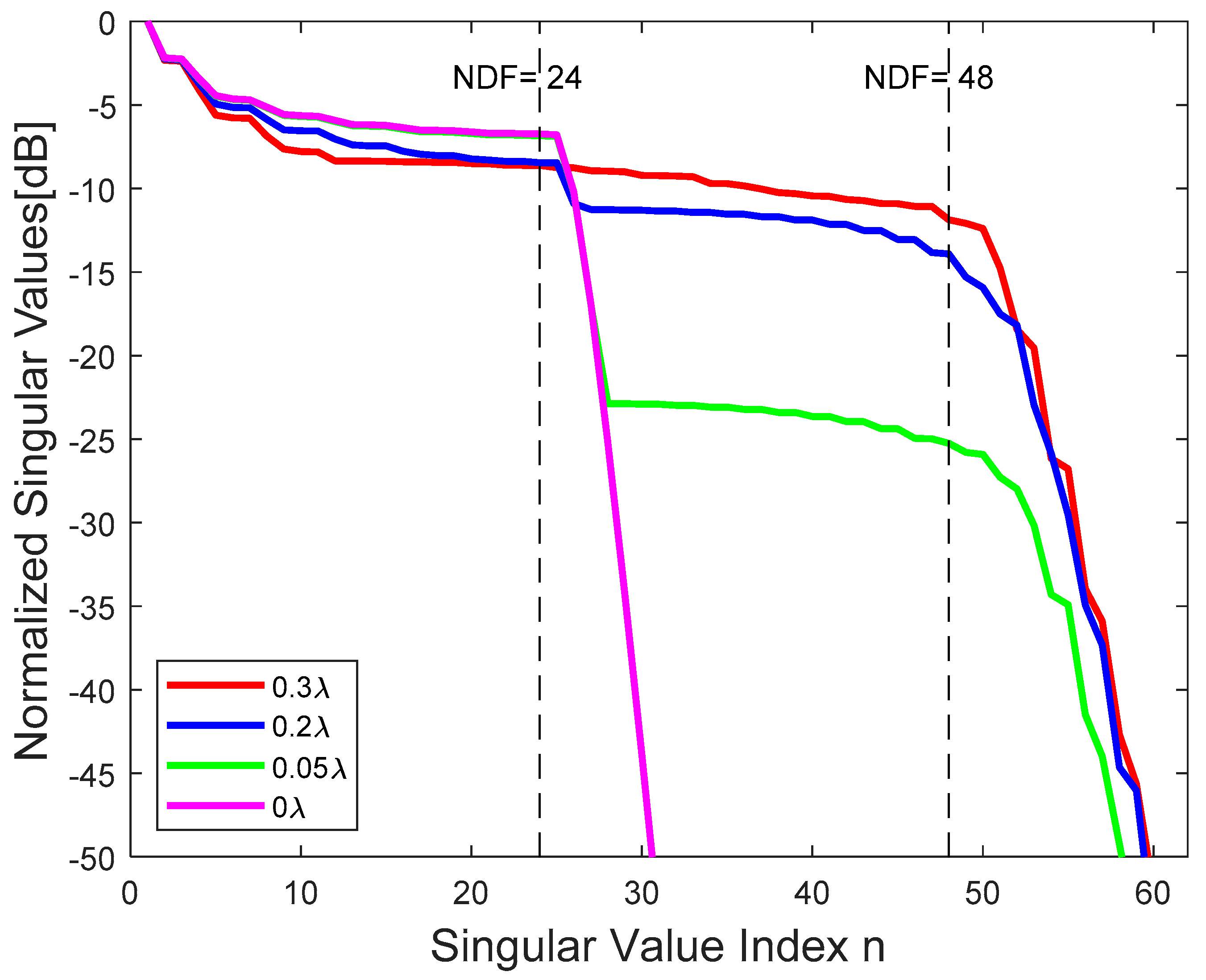
Figure 7 and Figure 8 confirm the estimation of Equation (32) numerically. As it occurs for the single strip case, we expect that two incident plane waves, with ${\theta }_i=0,\pi ,$ are enough to achieve the NDF of both strips.

In the numerical simulations, we consider the ID, as shown in Figure 6, composed of two equal strips with $a=3\lambda$. The upper bound of the whole NDF is $48$, according to Equation (32). The role of the distance $d$ in determining the NDF is considered in Figure 7. It is observed that the behavior of singular values does not change significantly for $d>0.3\lambda$, which can be identified as the minimum distance so that (32) holds.

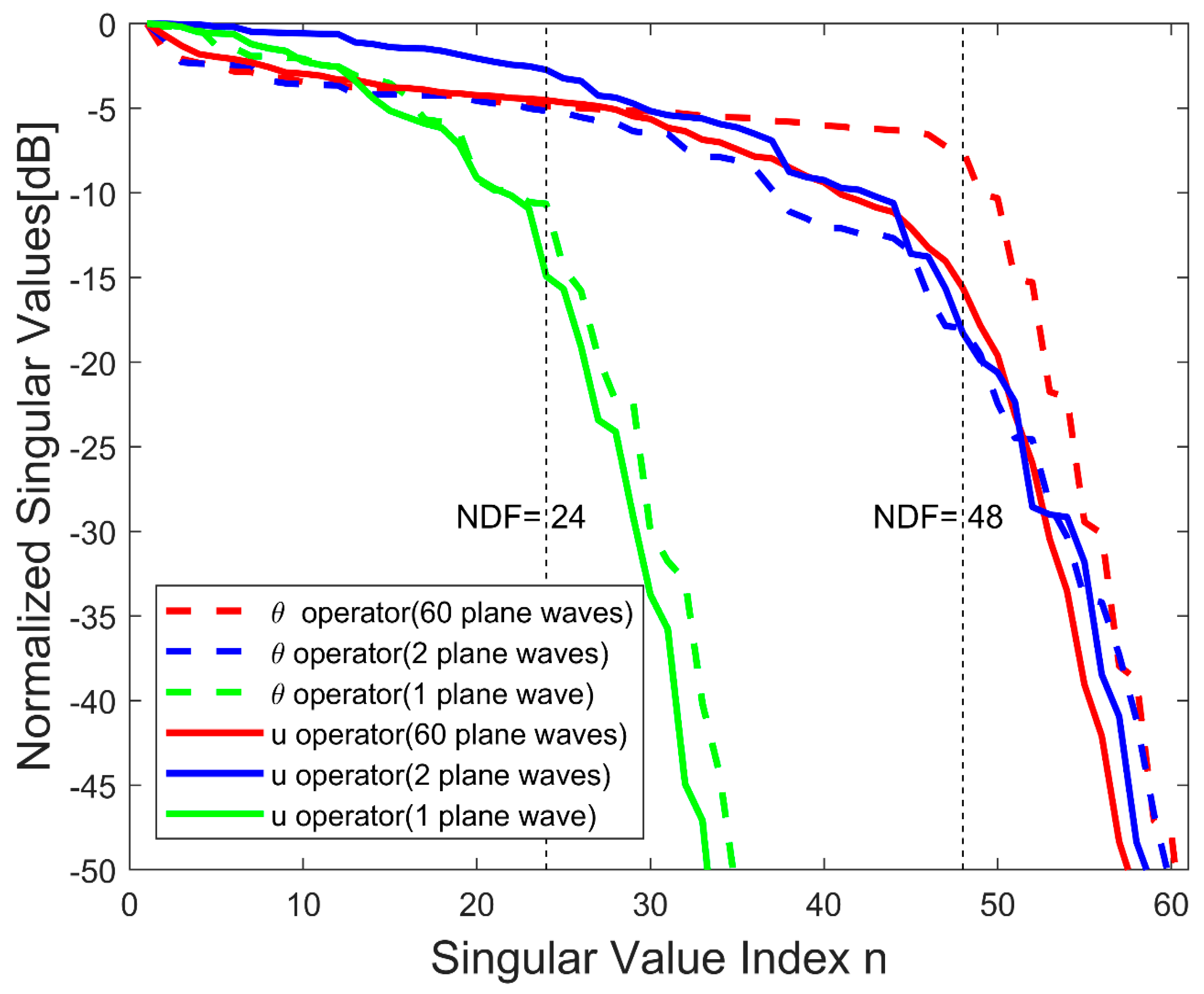
The normalized singular values of Equation (26) and the corresponding operator ${ℒ}_u$, written in terms of the $u_s,u_i$ variables, at different numbers of incident plane waves from different directions, are plotted in Figure 8. As can be seen, increasing the number of plane waves will not increase the NDF, and two plane waves are enough to achieve the whole NDF. The only difference between both operators ${ℒ}_{\theta }$ and ${ℒ}_u$ is the behavior of singular values; however, it can achieve the same NDF in both operators.

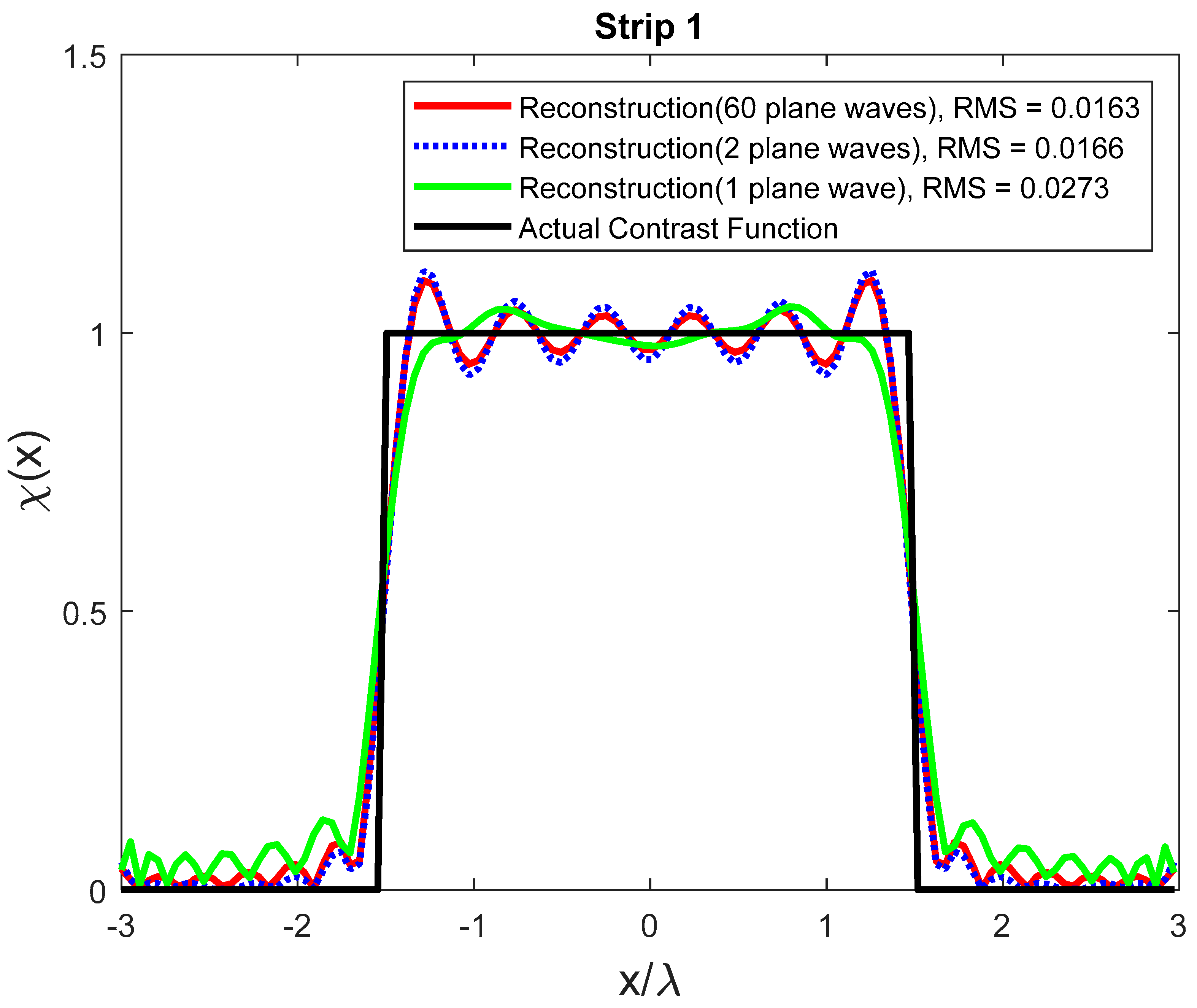
Figure 9 shows the same reconstructions as the previous section for a strip object inserted in the ID (strip 1) for different incident plane waves. As can be seen, the reconstructions by $60$ plane waves (red line) and by two plane waves (blue dotted line) nearly overlap. On the other hand, the reconstruction of one plane wave (green line) is markedly worst.

Figure 10 illustrates the effectiveness of reconstruction on strip 2. The results show that the reconstruction of strip 1 cannot affect strip 2.

5. Cross-Strip ID Geometry

This section is started by recalling the previous results to address the case of an ID composed of one strip lying along the x-axis and one strip lying along the y-axis, which can be named cross-strip geometry; furthermore, they are connected, as shown in Figure 11. The purpose of this section is to examine the NDF of the total scattered field, investigate the minimum number of independent plane waves to achieve the whole NDF, and introduce the optimal directions of plane waves while evaluating the role of their intersection on the NDF.

Recalling Equation (8), the far-field scattered by the horizontal strip and the vertical one is provided, respectively, by

$$E_{sh}\left({\theta }_s,{\theta }_i\right)={{\displaystyle \int }}_{-a}^a\chi \left(x\right)e^{j\beta x(\cos {\theta }_s-\cos {\theta }_i)}dx={ℒ}_x\left(\chi \left(x\right)\right)$$

(33)

and

$$E_{sv}\left({\theta }_s,{\theta }_i\right)={{\displaystyle \int }}_{-a}^a\chi \left(y\right)e^{j\beta y(\sin {\theta }_s-\sin {\theta }_i)}dy={ℒ}_y\left(\chi \left(y\right)\right)$$

(34)

We can consider the operator (35)

$$E_s\left({\theta }_s,{\theta }_i\right)=\left[\begin{array}{cc}{E}_{sh}\left({\theta }_s,{\theta }_i\right)& E_{sv}\left({\theta }_s,{\theta }_i\right)\end{array}\right]=\left[{ℒ}_x {ℒ}_y\right]\left[\begin{array}{c}\chi \left(x\right)\\ \chi \left(y\right)\end{array}\right]=ℒ \chi$$

(35)

This section’s mathematics is the same as Section 4, whereas now, the two strips are connected, and the four terms of the matrix (36) may be all significant. Hence, it may not be possible to ignore the two off-diagonal.

$${ℒ}^{+}ℒ\left(\chi \right)=\left[\begin{array}{c}{ℒ}_x^{+}{ℒ}_x {ℒ}_x^{+}{ℒ}_y \\ {ℒ}_y^{+}{ℒ}_x {ℒ}_y^{+}{ℒ}_y \end{array}\right]\left[\begin{array}{c}\chi \left(x\right)\\ \chi \left(y\right)\end{array}\right]$$

(36)

Consequently, if the area of intersection is significant, it may affect the NDF. Thus, the total NDF might be smaller than the summation of two NDF by

$$NDF<ND{F}_H+ND{F}_V$$

(37)

On the other hand, if the intersection area is just a point, it can be expected that it cannot affect the NDF significantly. Hence, we can expect that the total NDF may be approximately achieved by

$$NDF\approx ND{F}_H+ND{F}_V$$

(38)

In numerical simulations, we consider the ID shown in Figure 11, where the length $a$ of both strips is equal to $3\lambda$. The upper bound of the estimated total NDF is $48$, which is obtained by Equation (38), and the actual NDF is close to it.

Figure 12 shows the normalized singular values of (36) and the relevant operator ${ℒ}_u$ at different numbers of incident plane waves from different directions. Since two plane waves (${\theta }_i=0,\pi$) are optimal for one strip located on the x-axis, for symmetry reasons, we expect that two more incident plane waves for ${\theta }_i=\pi /2,3\pi /2$ should be added to achieve the whole NDF. The numerical results of Figure 12 confirm these expectations. As can be seen, the only difference between the two operators is the behavior of singular values, as the same results in previous sections.

Figure 13 illustrates a comparison between four plane waves from different directions. As can be seen, ${\theta }_i=\left[0,\pi /2,\pi ,3\pi /2\right]$ are the optimal directions since they allow to achieve the same number of NDF as for the $60$ plane waves case.

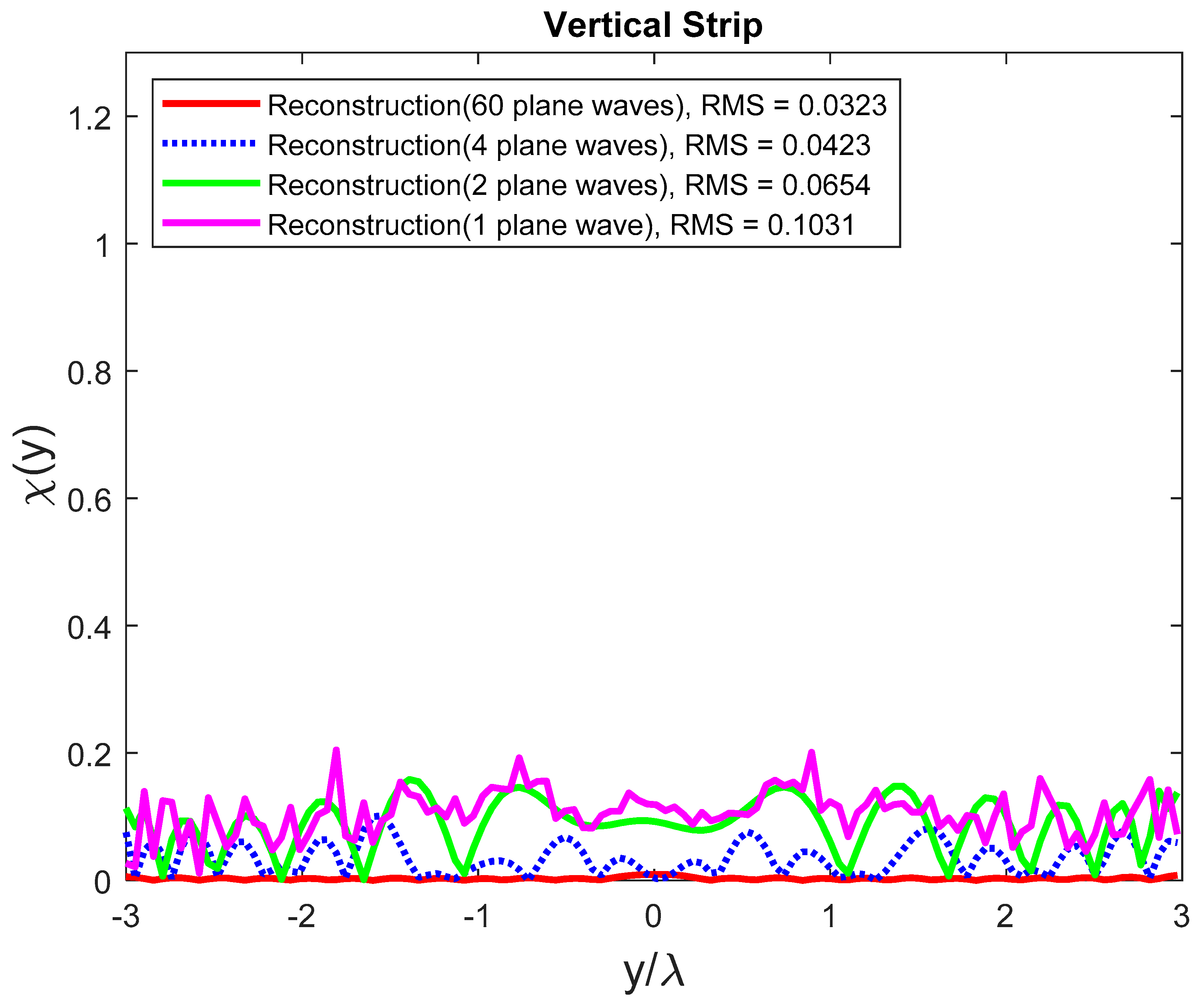
The same reconstructions as in previous sections of an object inserted in the ID for different incident plane waves are illustrated in Figure 14. The location of the scattering object within each ID is completely uninfluenced on the reconstruction results, as in the present approach, we take into account the whole set of objects embedded in the pertinent IDs. As can be seen, the reconstructions by $60$ plane waves and two plane waves nearly overlap. Moreover, the corresponding RMS is very close. On the other hand, the reconstructions with the incidence of two plane waves and one plane wave are less accurate.

The influence of the reconstruction of the horizontal strip on the vertical strip is shown in Figure 15. The results show that the reconstruction of the horizontal strip cannot affect the vertical strip.

6. Discussion and Conclusions

We have analyzed the NDF of scattered far fields for strip geometries at a single frequency, for the multi-view case, and both $\theta$ and $u$ observation variables. We theoretically estimated the NDF of scattered fields for one strip, two strips, and cross-strip using the Fourier transform and sampling theorem. Moreover, numerical simulations have shown that two incident plane waves for two strips and four incident plane waves for the cross-strip are adequate to achieve all NDF of these scattering geometries. Furthermore, we introduced the optimal directions of the plane waves for each geometry, that is, the minimum ones that allow us to achieve the same NDF than the total scattered fields. Besides, we observed that the same NDF is achieved independently on the observation variable, and the only difference is the behavior of singular values. Some numerical reconstructions at different numbers of the plane wave are presented for each geometry and confirm the expectations. These preliminary results about the NDF of the scattered fields and the possibility of choosing independent plane waves excitation are geometry dependent since the analytical properties of the linear operator to be considered are geometry dependent, too, and the extension to more general 2D geometries is under consideration.

The theoretical results about the NDF would impact the numerical effort of any imaging algorithm. In fact, the easiest way to find the contrast function of an object by scattered field data consists of the numerical inversion of the discretized version of the scattering operator (1) under the Born approximation. This amounts to inverting a matrix whose size is related to the electrical dimension of the object and the number of data points acquired at different observation angles for different plane wave incidences. It can reach a huge size for electrically large scattering objects when a λ/10 discretization step is adopted and if many scattered field data are considered. On the contrary, the NDF provides the maximum dimension of the subspace of the scattered fields that can be reconstructed by a robust linear inversion algorithm, and, at the same time, it provides the maximum dimension of the subspace of the corresponding contrast functions. Therefore, if appropriate basis functions for those subspaces were known to expand both data and unknowns, the resulting matrix would be reduced to a large extent to about the NDF × NDF size. As a result of the present investigation, where only the number of independent plane waves has been found, this final goal cannot be achieved yet, but a reduction of the size of the matrix to be inverted (and consequently, of the memory resources and the computing time) can be obtained. Quantitatively speaking, the overall reduction can be estimated as the ratio between a sufficiently large number of plane wave incidence, say 60 in our examples, and 2, or 4, that is the found minimum number of impinging plane waves. Of course, these time savings will reflect straightforwardly on any experimental imaging procedure to optimize the overall data acquisition time as well.