Translating Sentimental Statements Using Deep Learning Techniques


Abstract
1. Introduction
- The definitions of negative–positive pairs of sentimental statements with resembling semantics are proposed.
- To train the STM, the novel NPSS datasets are constructed with over 6 million negative–positive pairs of sentimental statements with resembling semantics.
- A series of tests are carried out to determine the translation outcomes, and further human evaluations on these outcomes are presented.
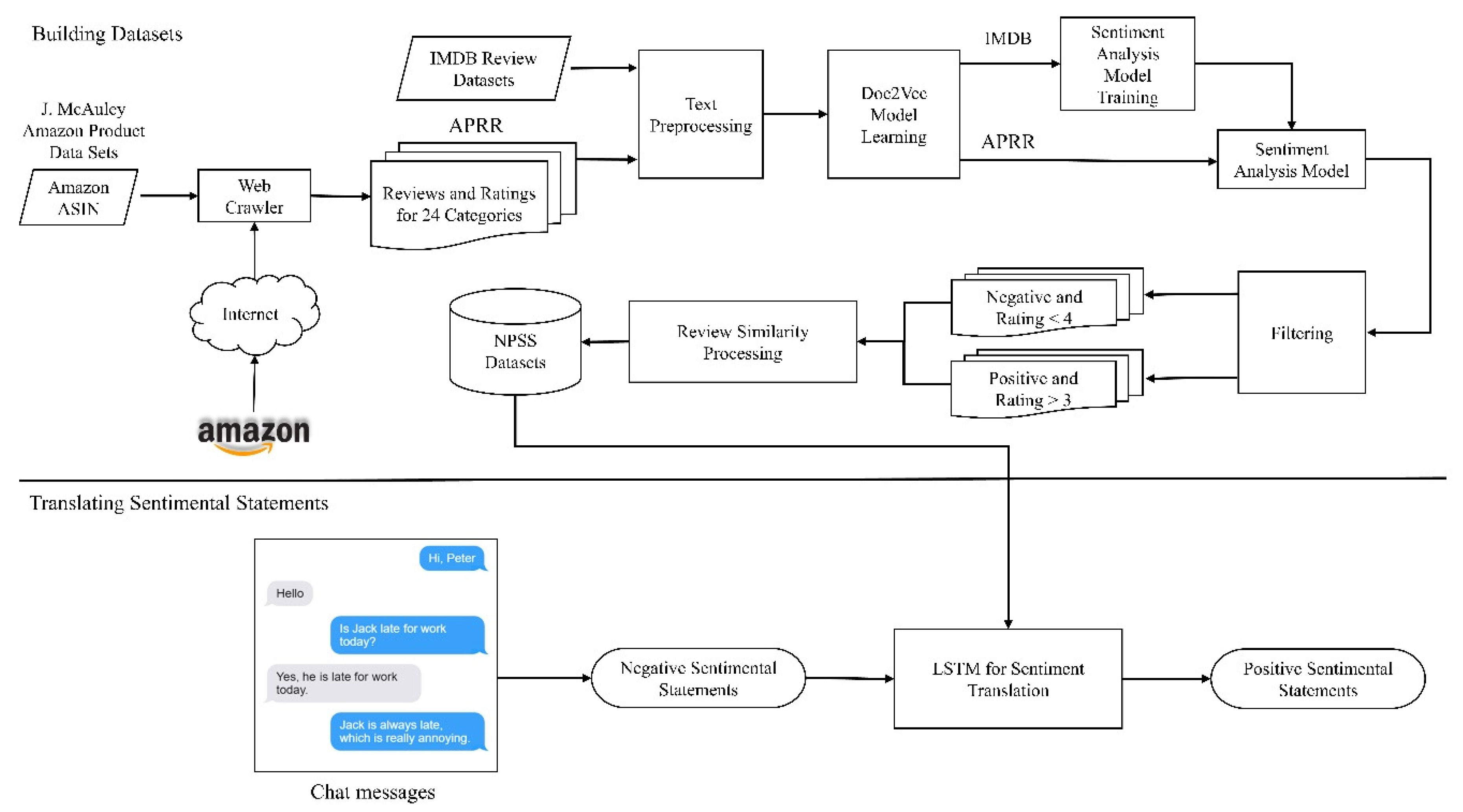
2. System Overview
3. Building Datasets
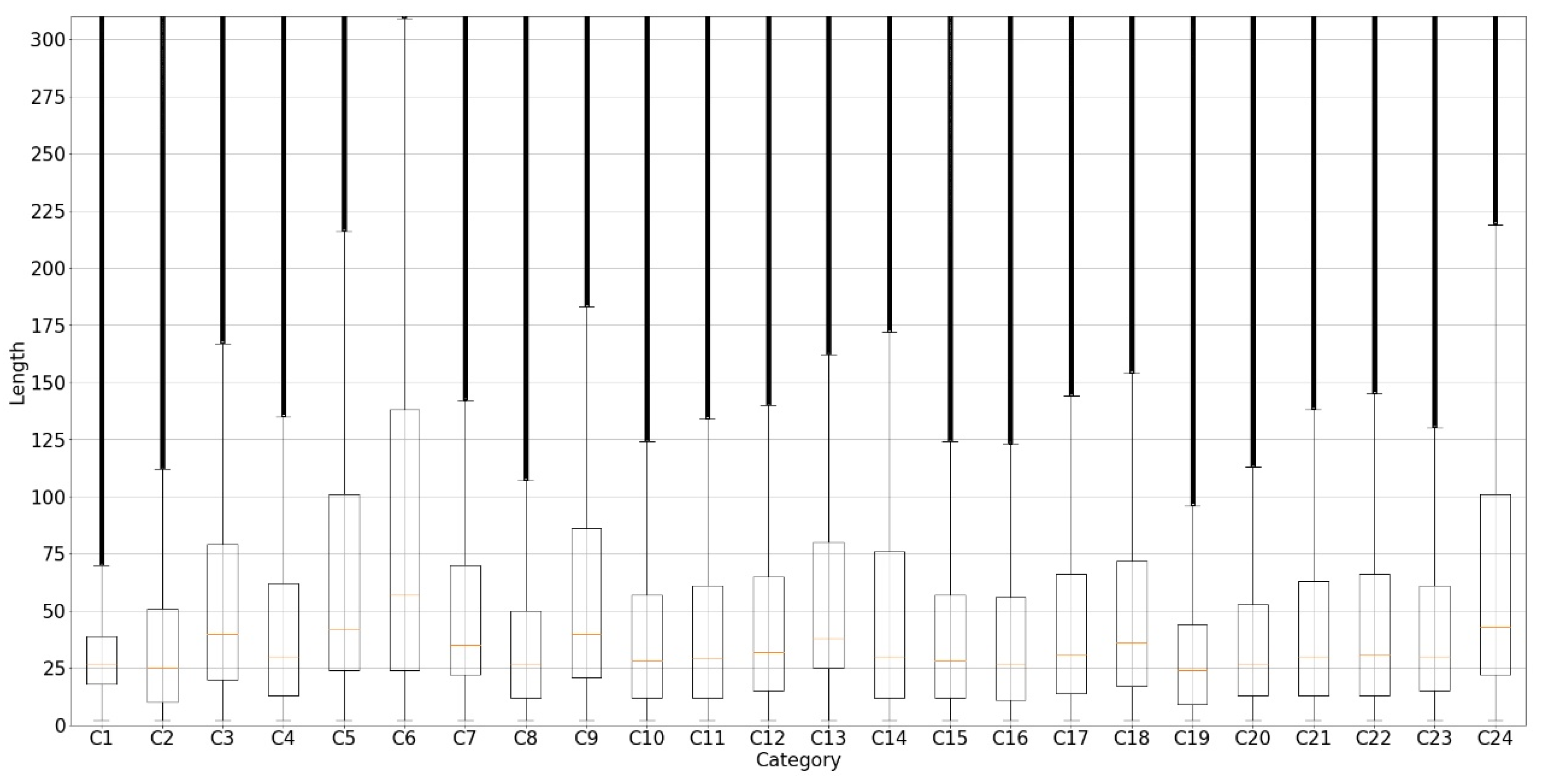
3.1. Datasets
3.2. Text Preprocessing
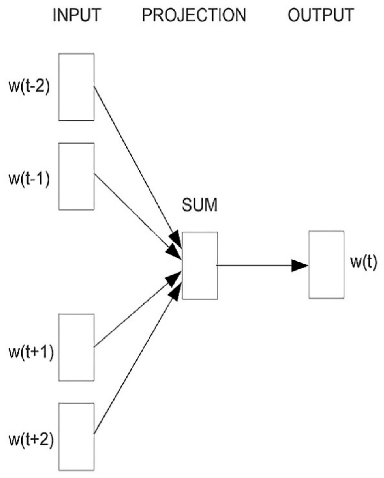
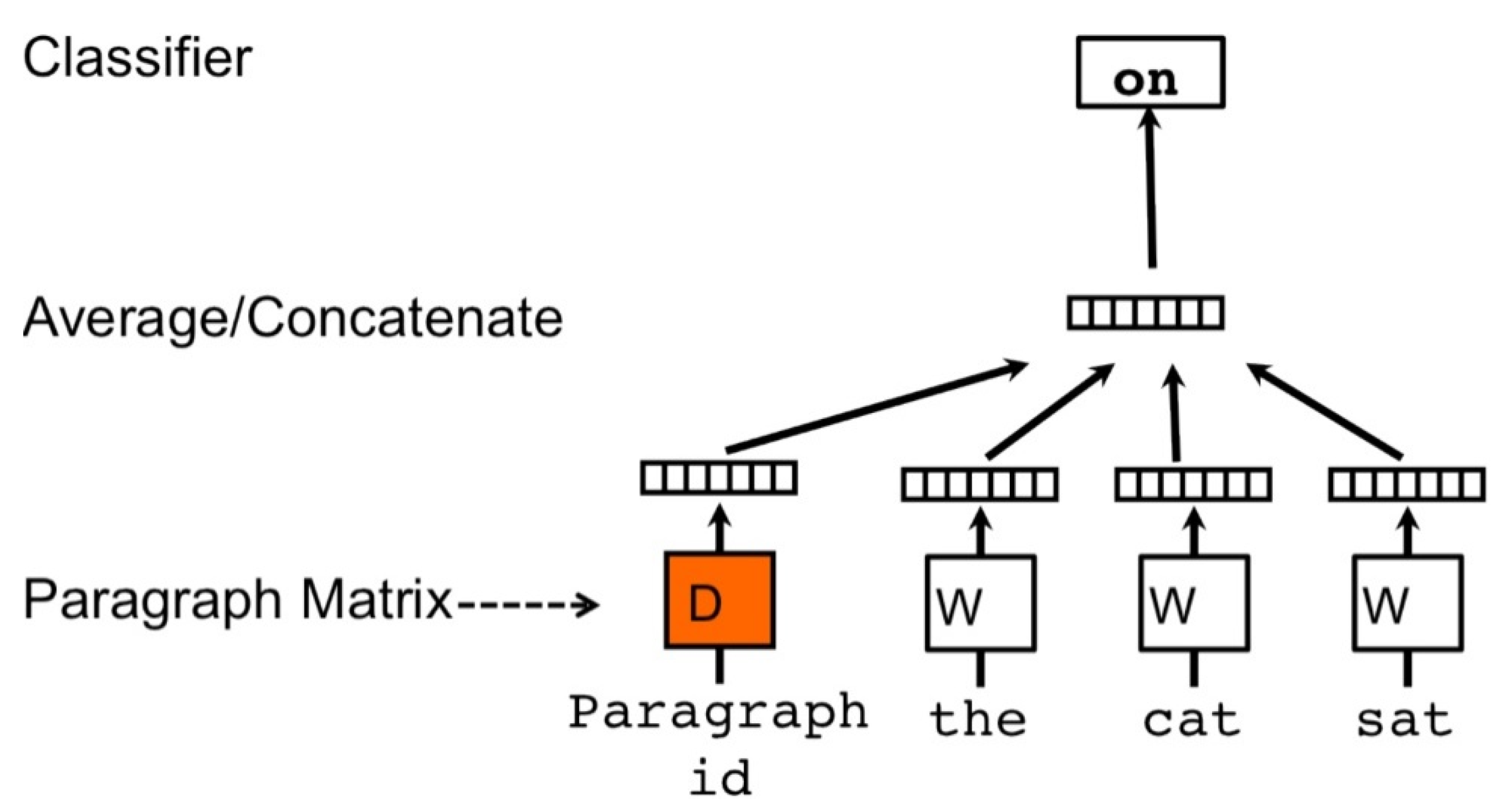
3.3. Doc2Vec Model Learning
3.3.1. Doc2Vec Model
3.3.2. Determining Dimensions and Architectures
3.4. Sentiment Analysis Model
3.5. Filtering
3.6. Review Similarity Processing
3.7. Negative–positive Sentimental Statement Datasets
4. Translating Sentimental Statements
4.1. LSTM
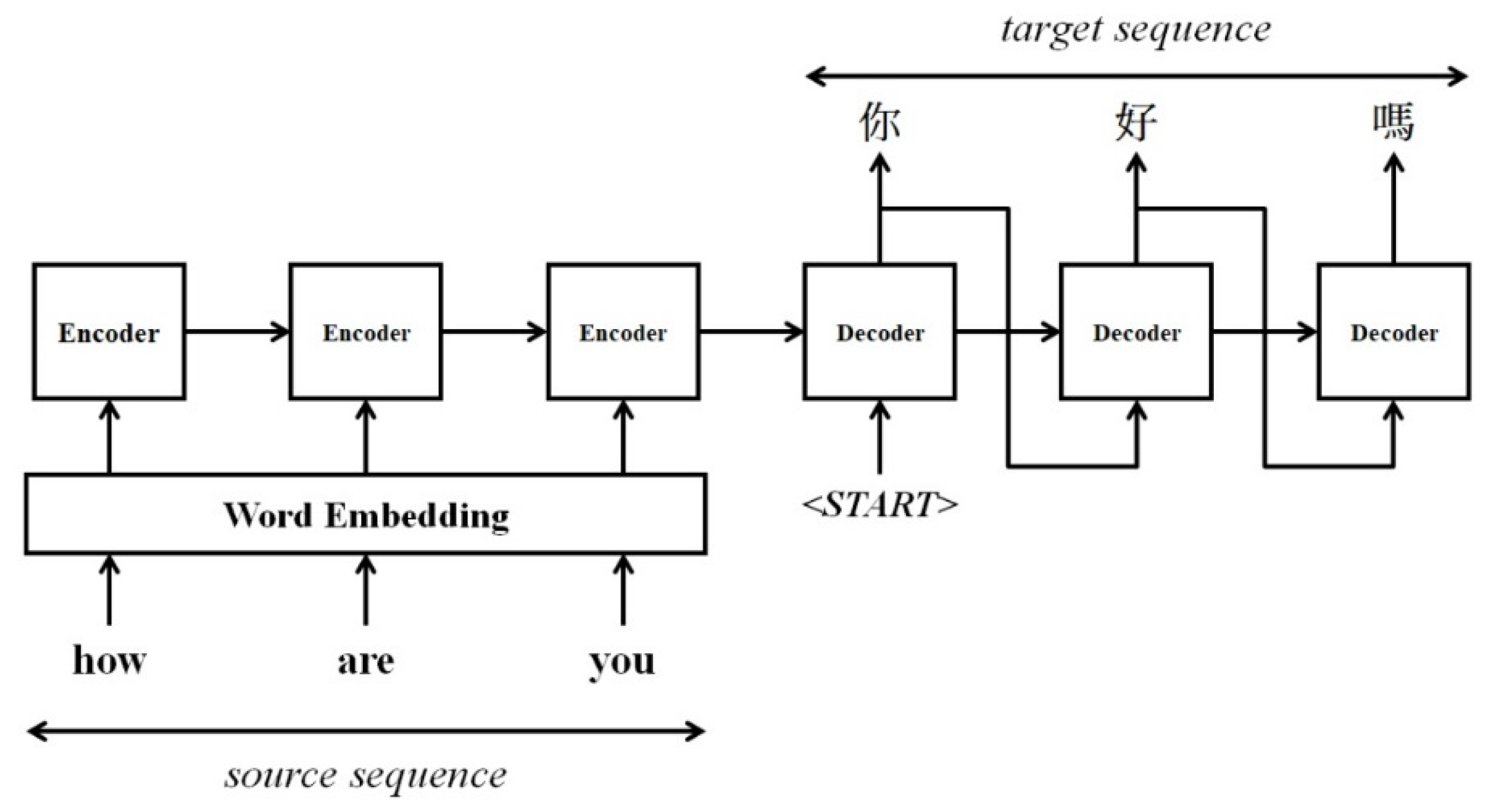
4.2. Seq2seq Model
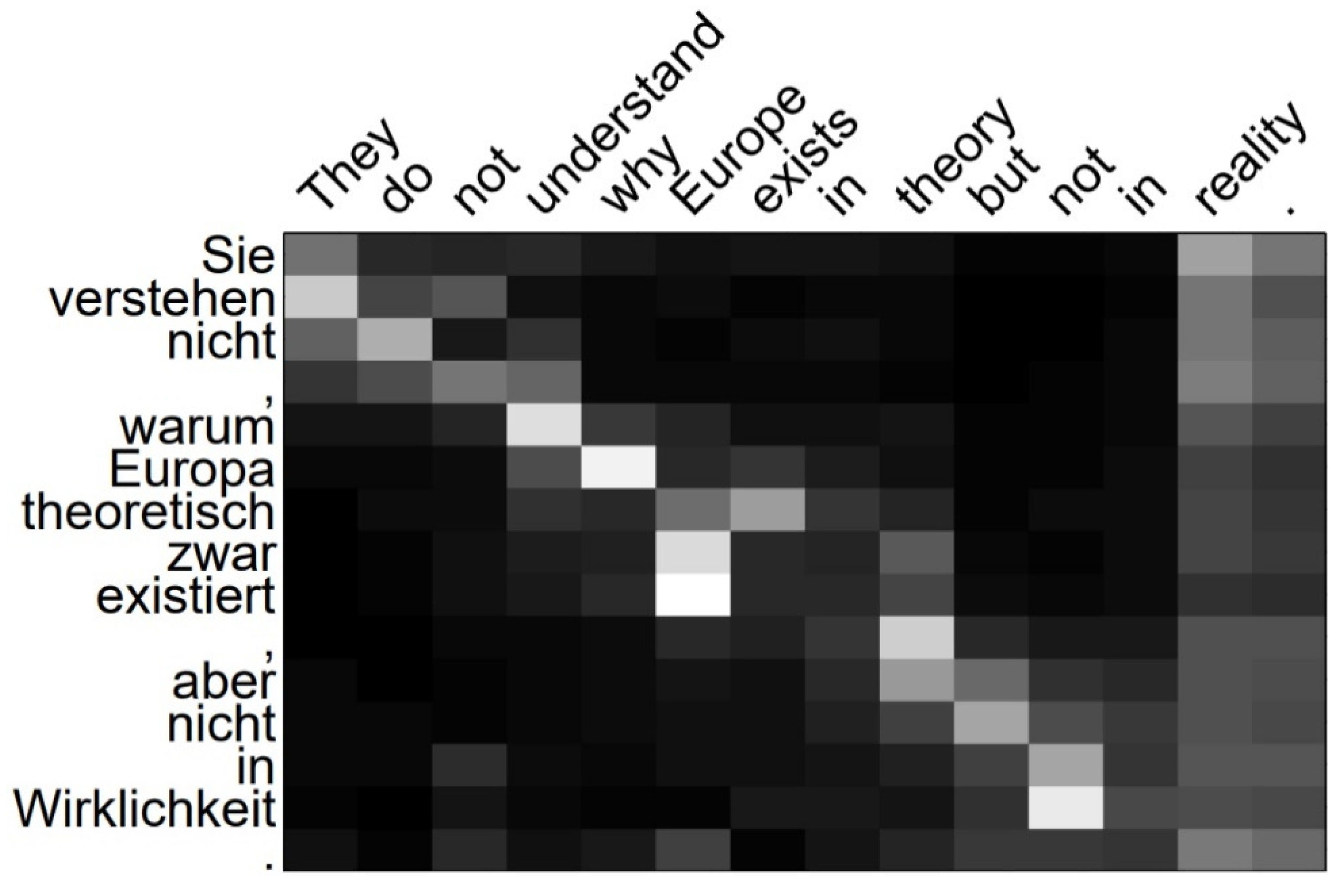
4.3. Attention Mechanism
4.4. Sentiment Translation Model
5. Experimental Results
5.1. Environments
- Batch size: 256
- Learning rate: 1.0
- Weights initialized from the uniform distribution [−0.1, 0.1]
- Optimizer: Stochastic Gradient Descent
- Gradient clipping threshold: 5
- Vocabulary size: 30,000
- Dropout rate: 0.2
- Epochs: 20
5.2. Evaluation Indicators
5.3. Case Comparisons in Experiment 1
5.4. Translated Sentimental Statements in Experiment 1
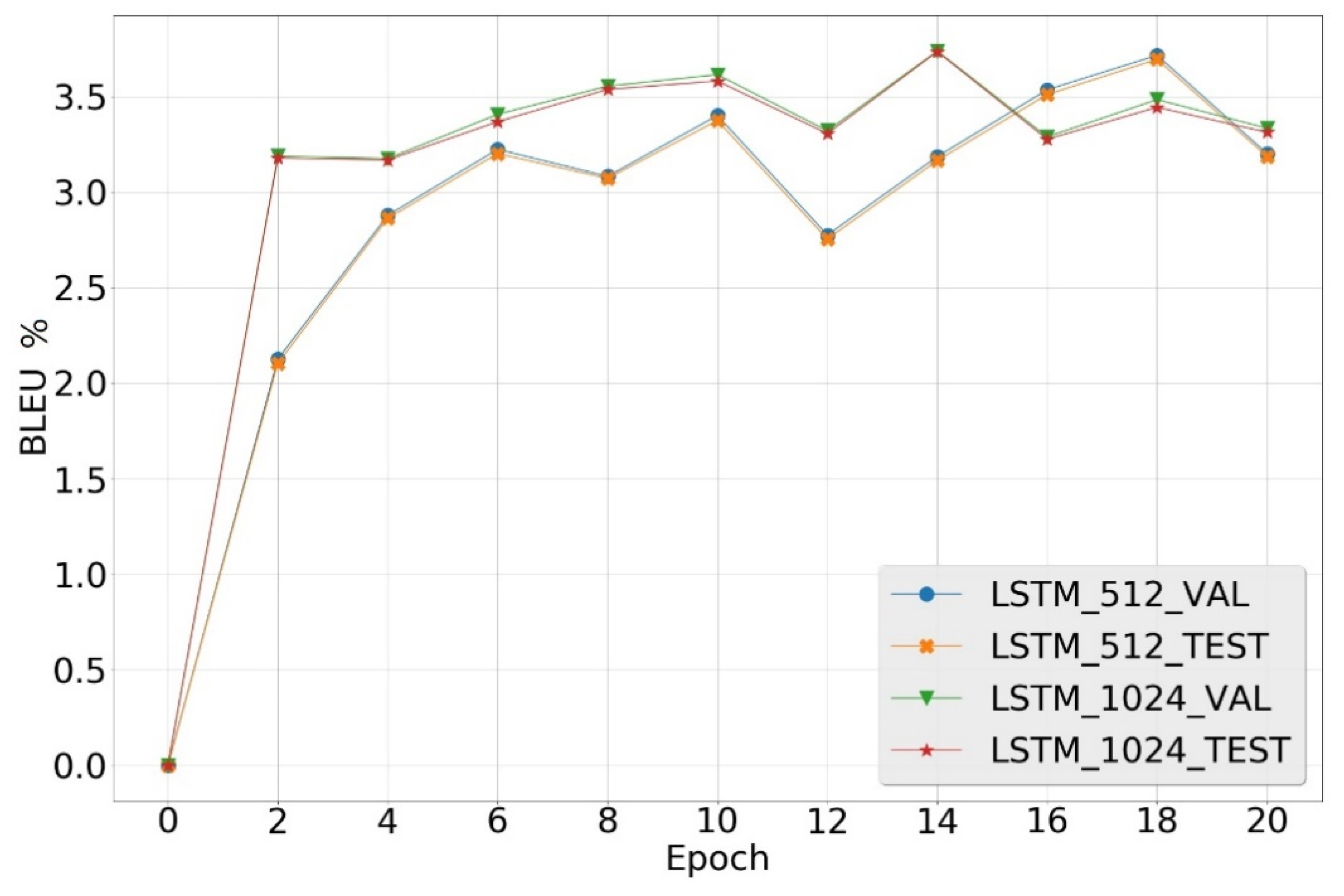
5.5. Results in Experiment 2
5.6. Human Assessments
6. Conclusions
- The Doc2Vec model can find semantically similar statements, but the statements could be contrary semantics. For example, “bad products” and “good products” are similar in semantics, but they are opposite and far from the negative-to-positive translation application.
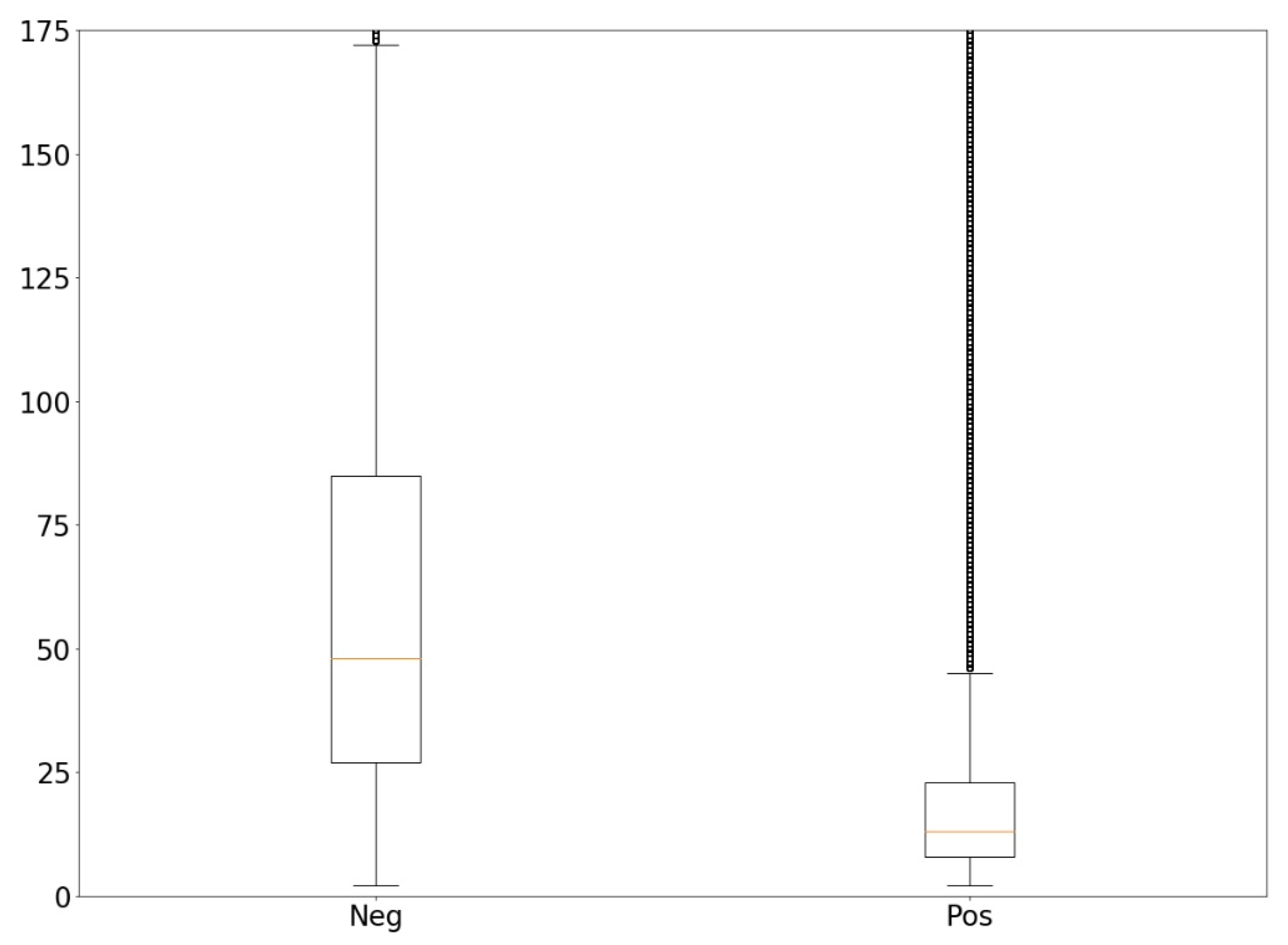
- While considering the similarity, the lengths of source statements and target statements should be considered. If their statement lengths are different too much (e.g., the length of a source/target statement is 100/10), it may cause a semantic loss in the translation.
Author Contributions
Funding
Data Availability Statement
Conflicts of Interest
References
- Li, H.; Lu, Z. Deep learning for information retrieval. In Proceedings of the 39th International ACM SIGIR Conference on Research and Development in Information Retrieval, Pisa, Italy, 17–21 July 2016; pp. 1203–1206. [Google Scholar]
- Yang, Y.; Yih, W.T.; Meek, C. Wikiqa: A challenge dataset for open-domain question answering. In Proceedings of the 2015 Conference on Empirical Methods in Natural Language Processing, Lisbon, Portugal, 17–21 September 2015; pp. 2013–2018. [Google Scholar]
- Joshi, A.; Fidalgo, E.; Alegre, E.; Fernández-Robles, L. SummCoder: An unsupervised framework for extractive text summarization based on deep auto-encoders. Expert Syst. Appl. 2019, 129, 200–215. [Google Scholar] [CrossRef]
- Hong, J.; Fang, M. Sentiment Analysis with Deeply Learned Distributed Representations of Variable Length Texts; Stanford University Report; Stanford University: Stanford, CA, USA, 2015. [Google Scholar]
- Huang, Y.F.; Li, Y.H. Sentiment translation model for expressing positive sentimental statements. In Proceedings of the International Conference on Machine Learning and Data Engineering, Taipei, Taiwan, 2–4 December 2019; pp. 79–84. [Google Scholar]
- Sutskever, I.; Vinyals, O.; Le, Q.V. Sequence to sequence learning with neural networks. In Advances in Neural Information Processing Systems; The MIT Press: Cambridge, MA, USA, 2014; pp. 3104–3112. [Google Scholar]
- Yu, L.; Zhang, W.; Wang, J.; Yu, Y. Seqgan: Sequence generative adversarial nets with policy gradient. In Proceedings of the 31st AAAI Conference on Artificial Intelligence, San Francisco, CA, USA, 4–9 February 2017. [Google Scholar]
- Vaswani, A.; Shazeer, N.; Parmar, N.; Uszkoreit, J.; Jones, L.; Gomez, A.N.; Polosukhin, I. Attention is all you need. In Advances in Neural Information Processing Systems; The MIT Press: Cambridge, MA, USA, 2017; pp. 5998–6008. [Google Scholar]
- He, R.; McAuley, J. Ups and downs: Modeling the visual evolution of fashion trends with one-class collaborative filtering. In Proceedings of the 25th International Conference on World Wide Web, Montreal, QC, Canada, 11–15 April 2016; pp. 507–517. [Google Scholar]
- McAuley, J.; Targett, C.; Shi, Q.; Van Den Hengel, A. Image-based recommendations on styles and substitutes. In Proceedings of the 38th International ACM SIGIR Conference on Research and Development in Information Retrieval, Santiago, Chile, 9–13 August 2015; pp. 43–52. [Google Scholar]
- Maas, A.L.; Daly, R.E.; Pham, P.T.; Huang, D.; Ng, A.Y.; Potts, C. Learning word vectors for sentiment analysis. In Proceedings of the 49th Annual Meeting of the Association for Computational Linguistics: Human Language Technologies, Portland, OR, USA, 19–24 June 2011; pp. 142–150. [Google Scholar]
- Le, Q.; Mikolov, T. Distributed representations of sentences and documents. In Proceedings of the International Conference on Machine Learning, Bejing, China, 22–24 June 2014; pp. 1188–1196. [Google Scholar]
- Hochreiter, S.; Schmidhuber, J. Long short-term memory. Neural Comput. 1997, 9, 1735–1780. [Google Scholar] [CrossRef] [PubMed]
- Hinton, G.E. Learning distributed representations of concepts. In Proceedings of the 8th Annual Conference of the Cognitive Science Society, Amherst, MA, USA, 15–17 August 1986. [Google Scholar]
- Mikolov, T.; Chen, K.; Corrado, G.; Dean, J. Efficient estimation of word representations in vector space. arXiv 2013, arXiv:1301.3781. [Google Scholar]
- Mikolov, T.; Sutskever, I.; Chen, K.; Corrado, G.S.; Dean, J. Distributed representations of words and phrases and their compositionality. In Advances in Neural Information Processing Systems; The MIT Press: Cambridge, MA, USA, 2013; pp. 3111–3119. [Google Scholar]
- Mikolov, T.; Yih, W.T.; Zweig, G. Linguistic regularities in continuous space word representations. In Proceedings of the 2013 Conference of the North American Chapter of the Association for Computational Linguistics: Human Language Technologies, Atlanta, GA, USA, 9–14 June 2013; pp. 746–751. [Google Scholar]
- Pennington, J.; Socher, R.; Manning, C. Glove: Global vectors for word representation. In Proceedings of the 2014 Conference on Empirical Methods in Natural Language Processing, Doha, Qatar, 25–29 October 2014; pp. 1532–1543. [Google Scholar]
- Bengio, Y.; Ducharme, R.; Vincent, P.; Jauvin, C. A neural probabilistic language model. J. Mach. Learn. Res. 2003, 3, 1137–1155. [Google Scholar]
- Rehurek, R.; Sojka, P. Software framework for topic modelling with large corpora. In Proceedings of the LREC 2010 Workshop on New Challenges for NLP Frameworks, Valletta, Malta, 22 May 2010. [Google Scholar]
- Gensim 3.8.3. Available online: https://pypi.org/project/gensim/ (accessed on 4 May 2020).
- Pang, B.; Lee, L. Opinion mining and sentiment analysis. Found. Trends Inf. Retr. 2008, 2, 1–135. [Google Scholar] [CrossRef]
- Sutskever, I.; Martens, J.; Hinton, G.E. Generating text with recurrent neural networks. In Proceedings of the 28th International Conference on Machine Learning, Montreal, QC, Canada, 28 June–2 July 2011; pp. 1017–1024. [Google Scholar]
- Cho, K.; Van Merriënboer, B.; Gulcehre, C.; Bahdanau, D.; Bougares, F.; Schwenk, H.; Bengio, Y. Learning phrase representations using RNN encoder-decoder for statistical machine translation. arXiv 2014, arXiv:1406.1078. [Google Scholar]
- Pascanu, R.; Mikolov, T.; Bengio, Y. On the difficulty of training recurrent neural networks. In Proceedings of the International Conference on Machine Learning, Atlanta, GA, USA, 16–21 June 2013; pp. 1310–1318. [Google Scholar]
- Mnih, V.; Heess, N.; Graves, A. Recurrent models of visual attention. In Advances in Neural Information Processing Systems; The MIT Press: Cambridge, MA, USA, 2014; pp. 2204–2212. [Google Scholar]
- Bahdanau, D.; Cho, K.; Bengio, Y. Neural machine translation by jointly learning to align and translate. arXiv 2014, arXiv:1409.0473. [Google Scholar]
- Luong, M.T.; Pham, H.; Manning, C.D. Effective approaches to attention-based neural machine translation. arXiv 2015, arXiv:1508.04025. [Google Scholar]
- Blei, D.M.; Ng, A.Y.; Jordan, M.I. Latent dirichlet allocation. J. Mach. Learn. Res. 2003, 3, 993–1022. [Google Scholar]
- Papineni, K.; Roukos, S.; Ward, T.; Zhu, W.J. BLEU: A method for automatic evaluation of machine translation. In Proceedings of the 40th Annual Meeting on Association for Computational Linguistics, Philadelphia, PA, USA, 6–12 July 2002; pp. 311–318. [Google Scholar]
- Chen, S.F.; Goodman, J. An empirical study of smoothing techniques for language modeling. Comput. Speech Lang. 1999, 13, 359–394. [Google Scholar] [CrossRef]
- Qian, X.; Zhong, Z.; Zhou, J. Multimodal machine translation with reinforcement learning. arXiv 2018, arXiv:1805.02356. [Google Scholar]
- Mawardi, V.C.; Susanto, N.; Naga, D.S. Spelling correction for text documents in Bahasa Indonesia using finite state automata and Levinshtein distance method. Proc. MATEC Web Conf. 2018, 164, 01047. [Google Scholar] [CrossRef]
- Chen, X.; Lawrence Zitnick, C. Mind’s eye: A recurrent visual representation for image caption generation. In Proceedings of the IEEE Conference on Computer Vision and Pattern Recognition, Boston, MA, USA, 7–12 June 2015; pp. 2422–2431. [Google Scholar]
- Vinyals, O.; Toshev, A.; Bengio, S.; Erhan, D. Show and tell: A neural image caption generator. In Proceedings of the IEEE Conference on Computer Vision and Pattern Recognition, Boston, MA, USA, 7–12 June 2015; pp. 3156–3164. [Google Scholar]
- Xu, K.; Ba, J.; Kiros, R.; Cho, K.; Courville, A.; Salakhudinov, R.; Bengio, Y. Show, attend and tell: Neural image caption generation with visual attention. In Proceedings of the International Conference on Machine Learning, Lille, France, 6–11 July 2015; pp. 2048–2057. [Google Scholar]
- Li, J.; Galley, M.; Brockett, C.; Spithourakis, G.P.; Gao, J.; Dolan, B. A persona-based neural conversation model. arXiv 2016, arXiv:1603.06155. [Google Scholar]
- Galley, M.; Brockett, C.; Sordoni, A.; Ji, Y.; Auli, M.; Quirk, C.; Dolan, B. DeltaBLEU: A discriminative metric for generation tasks with intrinsically diverse targets. arXiv 2015, arXiv:1506.06863. [Google Scholar]


| Categories | No. of Products | Ratings 4~5 | Ratings 1~3 | No. of Reviews | |
|---|---|---|---|---|---|
| C1 | Apps for Android | 13,147 | 2,006,327 | 778,726 | 2,785,053 |
| C2 | Automotive | 1817 | 709,782 | 145,202 | 854,984 |
| C3 | Baby | 6759 | 1,276,168 | 355,542 | 1,631,710 |
| C4 | Beauty | 10,825 | 2,533,868 | 712,946 | 3,246,814 |
| C5 | Book | 365,156 | 25,550,896 | 5,001,205 | 30,552,101 |
| C6 | CDs and Vinyl | 64,443 | 3,202,221 | 495,215 | 3,697,436 |
| C7 | Cell Phones and Accessories | 10,396 | 2,038,401 | 869,234 | 2,907,635 |
| C8 | Clothing Shoes and Jewelry | 22,787 | 4,473,465 | 1,172,548 | 5,646,013 |
| C9 | Electronics | 62,857 | 8,698,745 | 2,683,703 | 11,382,448 |
| C10 | Grocery and Gourmet Food | 8560 | 1,962,621 | 386,246 | 2,348,867 |
| C11 | Health and Personal Care | 18,458 | 4,924,158 | 1,240,566 | 6,164,724 |
| C12 | Home and Kitchen | 28,222 | 6,561,360 | 1,756,013 | 8,317,373 |
| C13 | Kindle Store | 61,929 | 2,788,628 | 647,101 | 3,435,729 |
| C14 | Movies and TV | 50,576 | 6,487,984 | 1,425,056 | 7,913,040 |
| C15 | Musical Instruments | 898 | 334,020 | 55,339 | 389,359 |
| C16 | Office Products | 2329 | 1,045,263 | 255,911 | 1,301,174 |
| C17 | Patio Lawn Garden | 954 | 464,412 | 122,039 | 586,451 |
| C18 | Pet Supplies | 8510 | 2,763,138 | 792,482 | 3,555,620 |
| C19 | Reviews Amazon Instant Video | 20,425 | 943,180 | 199,980 | 1,143,160 |
| C20 | Reviews Digital Music | 263,648 | 1,600,171 | 151,627 | 1,751,798 |
| C21 | Sports and Outdoors | 18,296 | 3,590,097 | 750,991 | 4,341,088 |
| C22 | Tools and Home Improvement | 10,097 | 2,261,018 | 512,217 | 2,773,235 |
| C23 | Toys and Games | 11,906 | 1,962,085 | 435,060 | 2,397,145 |
| C24 | Video Games | 8160 | 759,230 | 237,912 | 997,142 |
| All | 1,071,155 | 88,937,238 | 21,182,861 | 110,120,099 |
| Dimensions | Architectures | NPS | NS | NP | PS |
|---|---|---|---|---|---|
| 100 | DBOW | 89.32 | 89.58 | 89.56 | 89.58 |
| DMM | 87.32 | 87.60 | 87.13 | 86.78 | |
| DMC | 82.85 | 81.64 | 83.36 | 83.56 | |
| DBOW + DMM | 89.54 | 89.56 | 89.67 | 89.68 | |
| DBOW + DMC | 89.35 | 89.55 | 89.61 | 89.56 | |
| DMM + DMC | 86.58 | 86.60 | 86.48 | 86.24 | |
| 150 | DBOW | 89.20 | 89.15 | 89.36 | 89.26 |
| DMM | 87.82 | 87.89 | 87.73 | 87.64 | |
| DMC | 81.80 | 82.54 | 83.03 | 83.26 | |
| DBOW + DMM | 89.40 | 89.56 | 89.76 * | 89.60 | |
| DBOW + DMC | 89.24 | 89.27 | 89.45 | 89.38 | |
| DMM + DMC | 86.16 | 86.60 | 86.18 | 86.31 | |
| 250 | DBOW | 89.21 | 89.10 | 89.02 | 88.95 |
| DMM | 87.40 | 87.60 | 87.64 | 87.60 | |
| DMC | 80.95 | 82.04 | 82.56 | 82.77 | |
| DBOW + DMM | 89.39 | 89.32 | 89.26 | 89.35 | |
| DBOW + DMC | 89.18 | 89.12 | 89.02 | 88.98 | |
| DMM + DMC | 85.99 | 85.85 | 86.11 | 86.06 | |
| 400 | DBOW | 89.15 | 89.13 | 88.89 | 88.95 |
| DMM | 87.74 | 87.81 | 87.95 | 87.96 | |
| DMC | 76.88 | 80.49 | 73.61 | 73.65 | |
| DBOW + DMM | 89.27 | 89.17 | 89.13 | 89.01 | |
| DBOW + DMC | 89.21 | 89.16 | 89.05 | 88.94 | |
| DMM + DMC | 85.48 | 85.68 | 85.38 | 85.31 |
| Category | C1 | C2 | C3 | C4 | C5 | C6 | C7 | C8 |
| Accuracy | 88.74 | 89.19 | 88.58 | 88.12 | 87.63 | 87.96 | 88.17 | 87.85 |
| Category | C9 | C10 | C11 | C12 | C13 | C14 | C15 | C16 |
| Accuracy | 86.48 | 88.32 | 87.73 | 87.20 | 88.12 | 88.69 | 89.24 | 88.73 |
| Category | C17 | C18 | C19 | C20 | C21 | C22 | C23 | C24 |
| Accuracy | 89.14 | 87.92 | 89.08 | 88.70 | 87.82 | 88.12 | 88.16 | 89.10 |
| Case | Dataset | Perplexity | BLEU |
|---|---|---|---|
| LSTM(512) | Validation | 13.96 | 3.71% |
| Test | 13.98 | 3.69% | |
| LSTM(1024) | Validation | 12.68 | 3.74% |
| Test | 12.71 | 3.73% |
| Example 1 | |
| Source | Nice product. Overpriced. |
| Target | Nice product. |
| LSTM(512) | Nice product. |
| LSTM(1024) | Nice product. |
| Example 2 | |
| Source | This broke after two weeks just junk! |
| Target | Broke after months of use. I would buy again. |
| LSTM(512) | Broke after three uses. |
| LSTM(1024) | Broke after a few weeks but you get what you pay for. |
| Example 3 | |
| Source | Not very intuitive game play. Maybe I didn’t spend enough time on it but it seems slow and boring. Oh just fyi definitely not like a red alert type game. |
| Target | Fun game maybe not as cool as the first but still enjoyable. |
| LSTM(512) | I like it but it is a little slow. |
| LSTM(1024) | I like this game but it is not as intuitive as I thought it would be. Maybe a little slow. |
| Example 4 | |
| Source | Wobbly and rickety once put together. If the rack wobbles at all the dvd is fall out the back. Looks nice but doesn’t t function well. Returning. |
| Target | Stylish looks nice. Easy to put together. |
| LSTM(512) | Looks nice and is sturdy. |
| LSTM(1024) | Looks good but wobbles a lot. |
| Example 1 | |
| Source | Horrible product. Broke within a month. |
| Target | Great product! |
| LSTM(512) | Good quality and fit. |
| LSTM(1024) | Good quality and fit right. |
| Example 2 | |
| Source | Sickening scent. Smells completely different from the dove hairsprays I used previously. |
| Target | Best smelling hairspray ever! |
| LSTM(512) | Smells great. |
| LSTM(1024) | Love the scent. |
| Example 3 | |
| Source | Cheap and weak. Got weeks out of it. |
| Target | Got here days later it is good. |
| LSTM(512) | Got it weeks ago and it works great! |
| LSTM(1024) | Got it for a good price. |
| Example 4 | |
| Source | The range is too short for my use. I set up the unit in the living room with the hopes of controlling my cable box from another room. It works as long as the remote is close enough. At about feet, it is intermittent at best. |
| Target | Range is a little short at around feet but works great closer. |
| LSTM(512) | Works great. The remote is a little short but it works. |
| LSTM(1024) | Works great with my directv box. |
| Dataset | Perplexity | BLEU |
|---|---|---|
| 20% | 7.00 | 9.92% |
| 40% | 6.83 | 8.12% |
| 60% | 10.23 | 5.41% |
| 80% | 10.93 | 4.62% |
| 100% | 12.71 | 3.73% |
| Level | Input | Output |
|---|---|---|
| A | why not, you stupid bastard. | why not? |
| B | learning is painful, hate it. | learning so much. |
| C | you are hard to communicate. | easy to use and easy to hookup. |
| D | can’t sleep. i really hate sleepless nights. | i can’t sleep without it. |
| E | don’t bother me. | didn’t work for me. |
| Dataset | A | B | C | D | E | Score |
|---|---|---|---|---|---|---|
| 20% | 2 | 9 | 29 | 6 | 4 | 15.25 |
| 40% | 0 | 13 | 29 | 2 | 5 | 14.25 |
| 60% | 1 | 15 | 25 | 1 | 8 | 15.00 |
| 80% | 1 | 11 | 24 | 5 | 9 | 13.75 |
| 100% | 1 | 10 | 27 | 3 | 9 | 13.50 |
Publisher’s Note: MDPI stays neutral with regard to jurisdictional claims in published maps and institutional affiliations. |
© 2021 by the authors. Licensee MDPI, Basel, Switzerland. This article is an open access article distributed under the terms and conditions of the Creative Commons Attribution (CC BY) license (http://creativecommons.org/licenses/by/4.0/).
Share and Cite
Huang, Y.-F.; Li, Y.-H. Translating Sentimental Statements Using Deep Learning Techniques. Electronics 2021, 10, 138. https://doi.org/10.3390/electronics10020138
Huang Y-F, Li Y-H. Translating Sentimental Statements Using Deep Learning Techniques. Electronics. 2021; 10(2):138. https://doi.org/10.3390/electronics10020138
Chicago/Turabian StyleHuang, Yin-Fu, and Yi-Hao Li. 2021. "Translating Sentimental Statements Using Deep Learning Techniques" Electronics 10, no. 2: 138. https://doi.org/10.3390/electronics10020138
APA StyleHuang, Y.-F., & Li, Y.-H. (2021). Translating Sentimental Statements Using Deep Learning Techniques. Electronics, 10(2), 138. https://doi.org/10.3390/electronics10020138