Article

Fractional Order Adaptive Fast Super-Twisting Sliding Mode Control for Steer-by-Wire Vehicles with Time-Delay Estimation

1
School of Automobile and Traffic Engineering, Wuhan University of Science and Technology, Wuhan 430065, China
2
School of Energy Engineering, Huanghuai University, Zhumadian 463000, China
*
Author to whom correspondence should be addressed.
Electronics 2021, 10(19), 2424; https://doi.org/10.3390/electronics10192424
Submission received: 19 August 2021 / Revised: 17 September 2021 / Accepted: 2 October 2021 / Published: 5 October 2021
(This article belongs to the Section Systems & Control Engineering)

Abstract

:
It is difficult to model and determine the parameters of the steer-by-wire (SBW) system accurately, and the perturbation is variable with complex and changeable tire–road conditions. In order to improve the control performance of the vehicle SBW system, an adaptive fast super-twisting sliding mode control (AFST-SMC) scheme with time-delay estimation (TDE) is proposed. The proposed scheme uses TDE to acquire the lumped dynamics in a simple way and establishes a practical model-free structure. Then, a fractional order (FO) sliding mode surface and a fast super-twisting sliding mode control structure were designed on the basic super-twisting sliding mode to ensure fast convergence and high control accuracy. Since the uncertain boundary information of the actual system is unknown, a novel adaptive algorithm is proposed to regulate the control gain based on the control errors. Theoretical analysis concerning system stability is given based on the Lyapunov theory. Finally, the effectiveness of the method is verified through comparative experiments. The results show that the proposed TDE-AFST-FOSMC control scheme has the advantages of model-free, fast response and high accuracy.

1. Introduction

In recent years, the steer-by-wire (SBW) technology has been greatly developed and many research results have been achieved [1,2,3,4]. However, the SBW technology can not meet the requirements of practical application at present, and there is still a need to improve the reliability and control performance of SBW systems.
It is difficult to achieve high precision control for the SBW due to its complex dynamic characteristics and strong nonlinearity. Many factors affect the control performance of SBW simultaneously, such as system dynamics modeling, parameter perturbation, complicated road adhesion conditions, unexpected disturbance, and so on. Therefore, scholars have done a lot of work to develop applicable control algorithms. Certain progress has been made in control schemes based on sliding mode control, H2/H robust control, adaptive control, fuzzy control, neural network control and model predictive control [5,6,7,8,9].
Sliding mode control (SMC) is a variable structure control method, which has been widely used in various uncertain systems in recent years and has also achieved good results in the application of the SBW system. Various SMC algorithms have been developed to improve control performance. At first, the basic SMC was adopted in SBW, but it could not achieve the finite-time convergence of the error dynamics due to the linear sliding manifold. After that, different types of terminal sliding mode control and their variants were applied in the SBW system [10,11,12,13]. The nonlinear sliding manifold was constructed to accelerate the process of the system state approaching the equilibrium point and ensure finite-time reachability. Subsequently, in order to reduce chattering, the second-order sliding mode control was applied to the SBW system. The super-twisting sliding mode control component was used to guarantee strong robustness while alleviating the chattering phenomenon [14,15]. In practical applications, the boundary values of perturbations and parameter uncertainties are usually unknown. However, they are needed in the SMC controller’s design. Therefore, the adaptive algorithms are used to estimate the boundary values; then, the controller parameters can be adjusted accordingly [10,12].
In the steering process of vehicle operation, self-aligning torque and other disturbances act on the steering wheels. Moreover, the self-aligning torque is highly nonlinear and affected by many dynamic factors, which will greatly affect the steering tracking accuracy of SBW. If these disturbance torques can be estimated and compensated in feedforward control, the performance of the SBW controller will be greatly improved. In studies [11,16], an adaptive estimation law was employed to estimate the self-aligning torque coefficient. In [12], a Kalman filter was combined with an adaptive gain observer to calculate the self-aligning torque. The results proved that high tracking accuracy can be guaranteed via effectively estimating the self-aligning torque.
However, accurate estimation of the self-aligning torque requires accurate modeling of the vehicle and needs to take into account many effect factors, which are very difficult to achieve. In the aforementioned literature, simplified methods were employed. The influence of tires, suspensions and other characteristics was ignored. Consequently, the applicability of these methods is limited. It should also be noted that many parameters are involved in the SBW dynamics model, and these parameters may also have a certain degree of perturbation in the working process. These parameters are usually needed to complete the control. All the parameters need to be accurately measured for high-precision control performance of the SBW system, which is very difficult or even impossible.
In the control design of actual systems, uncertain parameters, unknown dynamics, and unexpected disturbances may be encountered. These unknown terms need to be estimated by appropriate methods. In the studies [17,18,19], Bresch-Pietri et al. investigated the adaptive control scheme for uncertain time-delay systems. The backstepping transformation is introduced to address the classic problems of equilibrium regulation under partial measurements, disturbance rejection, parameter or delay adaptation. Control strategies with time-delay on-line updating, parameters adaptation, input disturbance rejection, and distributed input estimation have been successively achieved. These research achievements have directive significance to the estimation of uncertain delay and unknown parameters for the time-delay system.
Another estimation technique is the so-called “time-delay estimation (TDE)”, which is generally used to estimate and cancel the nonlinear terms in the dynamics of a delay-free system. The TDE technique is originally proposed in areas of robotic control assuming that the disturbance does not change much from one sampling period to the next when the sampling rate is sufficiently high [20,21]. It has been successfully used to approximate the unknown dynamic model of robot manipulators [22,23,24]. In recent years, TDE has been adopted by many highly cited papers and has become a research hotspot [25,26,27].
In the TDE scheme, the system dynamics are composed of the desired dynamics and the remaining dynamics. The desired dynamics are known. The remaining dynamics are unknown including the uncertain dynamics and disturbances. Since the values of control input and system states at the past moment are known, the remaining dynamics at the past moment can be calculated. If the interval is sufficiently small, the difference of the remaining dynamics between the current moment and the past moment will be very small. So, the time-delayed remaining dynamics can be treated as the estimation of the current value. In this process, no specific system model is required. Therefore, TDE provides an attractive model-free property. However, TDE will inevitably introduce estimation error, which may lead to the decline of control performance. Therefore, a strong robust control scheme is needed to enhance nonlinear control based on TDE. Sliding mode control and its variants are widely combined with TDE schemes due to their strong robustness and simple form [23,24]. Kali et al. adopted the TDE-based super-twisting algorithm (STA) to control the uncertain manipulator and obtained good results successfully [28]. Therefore, in order to deal with the problem of self-aligning torque estimation and accurate acquisition of model parameters, time delay estimation is a good choice.
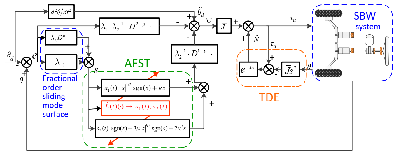
During the steering process, the disturbance torque applied to the steering system may change abruptly due to the variation of road adhesion conditions. If the disturbance torque cannot be compensated quickly, a large tracking error will be generated in the transient process. Therefore, on the basis of existing research, combined with TDE and super-twisting sliding mode, an adaptive fast super-twisting sliding mode controller based on TDE is proposed.
In this controller, TDE is adopted to solve the estimation problem of lumped uncertainty including system parameters and disturbances. The fast super-twisting structure and fractional sliding mode surface are employed to improve the tracking accuracy in the transition process of the system. According to the system state, the designed adaptive law can automatically adjust the super-twisting gain parameters. The proposed control scheme has the advantages of model-free, high tracking accuracy and strong robustness.

2. Plant Modeling

In the SBW system, the front wheels are driven by the steering motor through the steering gear. The rotation of the steering motor shaft is transmitted to the front wheels to perform the steering action, and Equations (1) and (2) are established.
θ ¨ f w θ ¨ p = θ ˙ f w θ ˙ p = θ f w θ p = 1 k 1
θ ¨ p θ ¨ s m = θ ˙ p θ ˙ s m = θ p θ s m = 1 k 2
where, k 1 , k 2 are the gear ratio. θ f w ,   θ p ,   θ s m are the rotation angles of the front wheel, the pinion and the steering motor shaft, respectively.
According to the driving torque and resistance torque around the rotation axis acting on the front wheels, Equation (3) is established.
J f w θ ¨ f w + B f w θ ˙ f w + τ F c s g n θ ˙ f w τ a + τ d = τ s
Equation (4) holds for the force analysis of the steering motor rotator.
J s m θ ¨ s m + B s m θ ˙ s m + τ p g k 2 = τ s m
J f w , J s m , B f w , B s m are the front wheel, steering motor inertia and viscous resistance coefficient. τ F C , τ a , τ d are the Coulomb friction torque, self-aligning torque and external disturbance torque of the wheel. τ s , τ p g , τ s m are the steering torque acting on the steering arm, the torque acting on the pinion, and the torque of the rotor of the steering motor, respectively. According to the transmission relationship, τ s = τ p g · k 1 , τ p g = τ s m · k 2 . Combined Equations (1)–(4), yield Equation (5).
J e θ ¨ s m + B e θ ˙ s m + τ F c k s g n θ ˙ f w τ a k + τ d k = τ s m
where, J e , B e are the equivalent inertia and equivalent viscous resistance coefficient of the steering system. J e = J s m + J f w / k 2 , B e = B s m + B f w / k 2 ,   k = k 1 · k 2 .
According to a DC motor’s equivalent circuit model, Equation (6) can be established.
u = L d i d t + R i + k e d θ s m d t τ s m = k m i
In a DC motor, L is usually very small and close to zero compared with R. Therefore, Equation (6) can be simplified as:
u = R i + k e θ ˙ s m τ s m = k m i
Combined (5), (7), θ s m abbreviated as θ , yield the dynamic Equation (8).
k m R u = J e θ ¨ + B e R + k e k m R θ ˙ + τ F c k s g n θ ˙ τ a k + τ d k
In the dynamics Equation (8), the steering device and steering motor are simplified to a certain extent in the modeling process. Compared with the actual steering system, the model has unmodeled dynamics. Moreover, Equation (8) involves parameters J s m , J f w , B s m , B f w , k m , k e , R , τ F C , in practical applications, it will be difficult to accurately determine the parameters. In addition, the self-aligning torque and the external disturbance torque are nonlinear, which are affected by many factors and are difficult to be accurately estimated. Therefore, it will face the problem of accurately determining the parameters and accurately estimating the self-aligning torque and external disturbance torque to achieve accurate tracking control of steering wheel angle with Equation (8).

3. Control Design of TDE-AFST-FOSMC

3.1. TDE Scheme

As aforementioned, the TDE technique directly utilizes the time-delayed information of the state variables and control input to estimate unknown dynamics and external disturbances. Only the value of state variables and control input at the past moment are required in the process. Therefore, it can be used to deal with the problem of accurately determining the model parameters and disturbance torque in the system (8). The specific implementation is as follows.
In order to facilitate the realization of the time-delay estimation scheme, a constant parameter J ¯ is introduced here, and the value of J ¯ can be determined by experiments. Rewrite system (8) as follows:
k m R u Control   input = J ¯ θ ¨ Desired   dynamics + J e J ¯ θ ¨ + B e R + k e k m R θ ˙ + τ F c k s g n θ ˙ τ a k + τ d k Remaining   dynamics
where, the desired dynamics are known, and the remaining dynamics are unknown. Rewrite system (9) as:
τ u = J ¯ θ ¨ + N
τ u = k m R u N =   J e J ¯ θ ¨ + B e R + k e k m R θ ˙ + τ F c k s g n θ ˙ τ a k + τ d k
In system (10), τ u is the control input, N is the remaining dynamics that need to be time-delay estimated. The value of J ¯ can be set according to the need, the optimal value can be determined by experiments.
In Equations (10) and (11), if N can be obtained timely and accurately, the control objectives can be easily achieved. The time delay estimation scheme can effectively satisfy acquisition of N by:
N ^ N t Δ t
where t is the delay time. When t is sufficiently small, the difference between N and N t Δ t will be small. Therefore, N t Δ t can be considered as an estimation of N . The lumped dynamics represented by N in (11) can be estimated using this method. Since t is very small, it does not lead to a large dynamics lag to make the system unstable [29]. In Equation (12), the TDE scheme uses the time delay value of N itself to obtain the estimated value of its current value. Since t is a small value, and it is generally selected as an integer multiple of the sampling period, this estimation scheme is effective for most systems.
According to Equations (10) and (12), we obtain:
N ^ N t Δ t = τ u t t J ¯ θ ¨ t Δ t
Therefore, the estimation value of N requires τ u t t and θ ¨ t t values. τ u t t can be acquired from the control input, while the θ ¨ t t can not be obtained directly without angular acceleration sensors. According to the existing literature, the following methods can be used to obtain θ ¨ t t [29,30,31].
θ ¨ t t =   θ t 2 θ t t + θ t 2 t / t 2 , t > t 1 θ ¨ t t = 0 , t t 1
where, t 1 2 t . In the case of small t , the bounded error generated by numerical differentiation in Equation (14) is close to zero and can be ignored. However, since t is small, t 2 is very small, the influence of noise is greatly amplified. In order to effectively suppress the influence of noise, small J ¯ or a low-pass filter can be selected.

3.2. Control Design of AFST-FOSMC

In order to achieve accurate tracking control under the condition of variable external disturbance and uncertain system parameters, inspired by reference [32], a novel adaptive fast super-twisting fractional-order sliding mode control (AFST-FOSMC) scheme is proposed in this paper.

3.2.1. Fast Super-twisting Algorithm with Fractional Order Sliding Mode

In the steering process, the desired steering motor shaft angle is defined as the reference angle θ d , which can be obtained from the desired front wheel angle θ f w using Equation (15). θ d is usually twice-differentiable due to common curves of roads.
θ d = θ f w k 1 k 2
We define the tracking error of the control system e as
e = θ θ d
The fractional order sliding manifold is designed as
s = λ 1 e + λ 2 D μ e
where, λ 1 , λ 2 > 0 ,   0 < μ < 1 . D μ f ( ) is the μ order fractional differential operator, more details can be found in reference [33].
Taking the time derivative, we yield
s ˙ = λ 1 e ˙ + λ 2 D μ + 1 e = λ 1 e ˙ + λ 2 D μ 1 e ¨
Referring to the method of literature [29], the control input is designed as
τ u = J ¯ v + N ^ v = θ ¨ d λ 1 λ 2 D 2 μ e 1 λ 2 D 1 μ a 1 ( t ) s 1 / 2 sgn ( s ) + κ s + a 2 ( t ) sgn ( s ) + 3 κ s 1 / 2 sgn ( s ) + 2 κ 2 s
where, a 1 ( t ) , a 2 ( t ) are the gain parameters regulated by the adaptive law.
Substituting Equation (19) into Equation (9), yield
J ¯ θ ¨ + N = J ¯ θ ¨ d λ 1 λ 2 D 2 μ e 1 λ 2 D 1 μ a 1 ( t ) s 1 / 2 sgn ( s ) + κ s + a 2 ( t ) sgn ( s ) + 3 κ s 1 / 2 sgn ( s ) + 2 κ 2 s + N ^
Rearrange and simplify, yield
θ ¨ θ ¨ d = λ 1 λ 2 D 2 μ e 1 λ 2 D 1 μ a 1 ( t ) s 1 / 2 sgn ( s ) + κ s + a 2 ( t ) sgn ( s ) + 3 κ s 1 / 2 sgn ( s ) + 2 κ 2 s + J ¯ 1 ( N ^ N )
Defined TDE error as ε = J ¯ 1 ( N ^ N ) , since θ ¨ θ ¨ d = e ¨ , we obtain
e ¨ = λ 1 λ 2 D 2 μ e 1 λ 2 D 1 μ a 1 ( t ) s 1 / 2 sgn ( s ) + κ s + a 2 ( t ) sgn ( s ) + 3 κ s 1 / 2 sgn ( s ) + 2 κ 2 s + ε
Taking the same μ 1 order differential for two ends of Equation (20), and multiply factor λ 2 , rearrange and simplify, we yield
λ 2 D μ 1 e ¨ + λ 1 e ˙ = a 1 ( t ) s 1 / 2 sgn ( s ) + κ s + a 2 ( t ) sgn ( s ) + 3 κ s 1 / 2 sgn ( s ) + 2 κ 2 s + λ 2 D μ 1 ε
Define ρ t   = λ 2 D μ ε , combine with Equation (18), rearranging Equation (21), we get the dynamic Equation (22) with super-twisting form.
s ˙ = a 1 ( t ) s 1 / 2 sgn ( s ) + κ s + φ φ ˙ = a 2 ( t ) sgn ( s ) + 3 κ s 1 / 2 sgn ( s ) + 2 κ 2 s + ρ ( t )
where a 1 ( t ) , a 2 ( t ) are the gain parameters, κ is the constant parameter.
Equation (22) is a variant super-twisting structure originated from the basic super-twisting. Compared with Equation (23), the power reaching law s 1 / 2 sgn ( s ) is replaced by the fast terminal reaching law s 1 / 2 sgn ( s ) + κ s in the improved super-twisting structure. As shown in Figure 1, the improved structure (22) can significantly accelerate the convergence of the sliding manifold under the same condition.
s ˙ = a 1 s 1 / 2 sgn ( s ) + φ φ ˙ = a 2 sgn ( s ) + f ( t )

3.2.2. Design of Adaptive Law

In the system dynamics Equation (22), the values of gain parameters a 1 t , a 2 t affect the quality of dynamic processes and need to be chosen reasonably. Due to the influence of system parameter perturbation and external disturbance torque, N in Equation (11) is constantly changing, and the delay estimation error ε = J ¯ 1 ( N ^ N ) is also constantly changing. Accordingly, the disturbance term ρ ( t ) = λ 2 D μ ε in system (22) is uncertain. According to the proof in references [28,31], when the delay time t is small enough, the delay estimation error ε is bounded and the time derivative ε ˙ is bounded. Since ρ ( t ) is the μ order differential of the time delay estimation error ε , ρ ( t ) is bounded too. Assume ρ ( t )   σ , fixed design scalar l 0 > 0 , select scalar function L ( t ) > max σ , l 0 , the gain parameters a 1 ( t ) , a 2 ( t ) could be chosen according to Equation (24) [34]:
a 1 ( t ) = a 1 L ( t ) a 2 ( t ) = a 2 L ( t )
where, a 1 > 0 , a 2 > 0 , are factors to be designed. The value of L ( t ) is determined by the adaptive law.
Inspired by reference [32], the gain parameter can be adjusted by an adaptive law to make it close to the tight upper bound of the uncertainty. So that, the sliding variable is maintained in a preset neighborhood, and accurate tracking of steering angle can be achieved under different working conditions. The adaptive law is proposed as shown in Equation (25):
L ˙ ( t ) =   η , L ( t ) L max λ L ( t ) ω s s 0 s 0 , L min < L ( t ) < L max ,   a n d     s s 0 ω s s 0 s 0 , L min < L ( t ) < L max ,   a n d     s > s 0 η , L ( t ) L min
where, η , ω , s 0 > 0 , 0 < λ L ( t ) < 1 , are parameters to be designed. The specific values can be adjusted according to the experimental results. According to the adaptive law, when L ( t ) is lower than the lower limit or higher than the upper limit, it increases or decreases at a constant rate η , so that it can be maintained within the upper and lower limits. When the sliding mode variable s exceeds the neighborhood defined by s0, the increase rate of L ( t ) is given by ω ( s s 0 ) / s 0 . The greater the deviation is, the greater L ˙ ( t ) is. When the sliding mode variable s is in the neighborhood limited by s0, L ( t ) slowly decreases at the rate of λ L ( t ) ω ( s s 0 ) / s 0 . So that the system states could be maintained in the neighborhood s s 0 .
The block diagram of our proposed TDE-based AFST-FOSMC control scheme is depicted in Figure 2.

3.3. System Stability Analysis

To facilitate the stability analysis of the system (22), coordinate transformations are performed as follows:
ξ = ξ 1 ξ 2 = L ( t ) ( s 1 / 2 sgn ( s ) + κ s ) φ
Taking the derivative of ξ , obtain
ξ ˙ 1 = L ( t ) ( 1 2 s 1 / 2 s ˙ + κ s ˙ ) = L ( t ) ( 1 2 s 1 / 2 + κ ) a 1 ( t ) s 1 / 2 sgn ( s ) + κ s + φ
ξ ˙ 2 = φ ˙ = a 2 ( t ) sgn ( s ) + 3 κ s 1 / 2 sgn ( s ) + 2 κ 2 s + ρ = ( 1 s 1 / 2 + 2 κ ) a 2 ( t ) ( s 1 / 2 sgn ( s ) + κ s ) + ρ
Rewrite system Equation (22) with ξ as system variable:
ξ ˙ 1 = L ( t ) ( 1 s 1 / 2 + 2 κ ) a 1 ( t ) 2 L ( t ) ξ 1 + 1 2 φ ξ ˙ 2 = L ( t ) ( 1 s 1 / 2 + 2 κ ) a 2 ( t ) L ( t ) ξ 1 + ρ ¯
where, ρ ¯ is defined as ρ ¯ = s 1 / 2 ρ L ( 1 + 2 κ s 1 / 2 ) , Equation (29) rewriting to matrix form, we obtain
ξ ˙ = D ( s ) ( A ξ + B ρ ¯ )
where, A = a 1 2 1 2 a 2 0 , B = 0 1 , D ( s ) = L ( t ) ( 1 s 1 / 2 + 2 κ ) .
Define a symmetric matrix P = p 1 p 2 p 2 p 3 , p 1 , p 3 > 0 , p 2 2 < p 1 p 3 , then P is a positive definite matrix. The Lyapunov function is constructed as V = ξ T P ξ , V is positive definite and radially unbounded. Taking derivation of V along the system trajectory, yield
V ˙ = ( ξ ˙ ) T P ξ + ξ T P ξ ˙ = [ D ( s ) ( A ξ + B ρ ¯ ) ] T P ξ + ξ T P [ D ( s ) ( A ξ + B ρ ¯ ) ] = D ( s ) [ ξ T ( A T P + P A ) ξ + ρ ¯ B T P ξ + ξ T P B ρ ¯ ] D ( s ) [ ξ T ( A T P + P A ) ξ + ξ T P B B T P ξ + ρ ¯ 2 ]
For
ξ 1   =   L ( s 1 / 2 sgn ( s ) + κ s )   = L s 1 / 2 ( 1 + κ s 1 / 2 ) ,  
ρ ¯   = s 1 / 2 L ( 1 + 2 κ s 1 / 2 ) ρ   ρ L ξ 1     ξ 1   ,
Then V ˙ D ( s ) [ ξ T ( A T P + P A ) ξ + ξ T P B B T P ξ + ξ 1 2 ] , select C =   1 0 , then
V ˙ D ( s ) [ ξ T ( A T P + P A + P B B T P + C T C ) ξ ] .
If the values of a 1 , a 2 make the positive definite symmetrix P satisfying inequality (31) exit, where ε 0 > 0 , then Equation (32) holds.
A T P + P A + P B B T P + C T C + ε 0 P < 0
V ˙ ε 0 s 1 / 2 L V 2 κ ε 0 L V
According to ξ 1   = L s 1 / 2 ( 1 + κ s 1 / 2 ) , there is L s 1 / 2 <   ξ 1   <   ξ , and λ min ( P ) ξ 2 V , we obtain s 1 / 2 V 1 / 2 ( λ min ( P ) L ) 1 / 2 , then Equation (32) can be reduced as V ˙ ε 0 L λ min ( P ) V 1 / 2 2 κ ε 0 L V . For L > l 0 , then V ˙ + η 1 V + η 2 V 1 / 2 0 , where η 1 = 2 κ ε 0 l 0 , η 2 = ε 0 l 0 λ min ( P ) . Based on the existing work in the literature [35], it is known that the system (30) achieves the second-order sliding mode motion in finite time Tr, ξ ( t ) = 0 holds and Tr satisfies Equation (33). According to the definition in Equation (26), s = 0 , φ = 0 hold. According to Equation (22), s ˙ = 0 holds too.
T r = 2 η 1 ln 1 + η 1 η 2 V 1 / 2 ( 0 )
According to the Bounded Real Lemma, inequality (31) is equivalent to the frequency domain constraint G 0 s < 1 , where the transfer function G 0 ( s ) : = C ( s I A ) 1 B = 1 / ( 2 s 2 + a 1 s + a 2 ) . The necessary condition is that a 2 > 1 to ensure G 0 s < 1 . Therefore, the value of a 1 , a 2 can refer to the literature [34] and choose as a 1 = 1.5 , a 2 = 1.1 , which will make the inequality (31) hold and make system (22) stable.

4. Experimental Verification
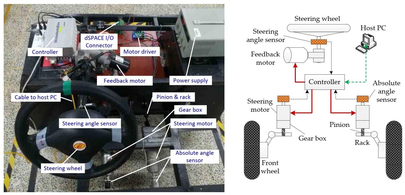
As shown in Figure 3, the SBW experimental plant is composed of steering motors, steering gears, front wheels, angle sensors and a controller. The steering angle sensor measures the driver’s steering command angle. The multi-ring absolute encoder measures the angular position of the steering motor shaft as a feedback signal. The dSPACE MAB is used as an SBW controller which receives the sensors’ angle signals and outputs the control signal. The host computer records the data in the experiment process. In the experiment, the controller receives the sensor’s data through the CAN bus, and the CAN bus rate is set as 500 kb/s. The encoder is set to timing mode, angular position data is sent to the controller every 50 microseconds. The relevant parameters used by the controller are shown in Table 1.
In order to verify the effectiveness of the control algorithm proposed in this paper, the setting condition experiments and simulation experiments are carried out on the experimental plant. The control accuracy and disturbance estimation performance of different algorithms are verified through experiments. In the experiment, the control algorithm for comparison is carried out under the same conditions. The results validated the effectiveness and the advantage of the proposed algorithm.

4.1. Control Algorithm for Comparison

The performance of time-delay estimation, fast super-twisting fractional order sliding mode and adaptive control law are verified in the experiments. In order to carry out comparative research, the traditional adaptive sliding mode control (ASMC), the super-twisting sliding mode control based on TDE (TDE-STSMC), the fast super-twisting fractional order sliding mode control based on TDE (TDE-FST-FOSMC) are selected as the controllers for comparative verification.
In order to facilitate the design of the comparison controller, the SBW system dynamic equation is arranged as follows. Substituting Equation (7) into Equation (5) and rearranging into state equation form, the steering system dynamic Equation (34) can be obtained.
x ˙ 1 = x 2 x ˙ 2 = g 0 ( x ) u + f 0 ( x ) + d
where, x = x 1 , x 2 T = θ s m , θ ˙ s m T , f 0 ( x ) = k m k e + B e R J e R x 2 τ F c s g n ( x 2 ) k J e , g 0 ( x ) = k m J e R . d is the lumped disturbance term, d = τ a x + τ d x + Δ p a r a m + Δ u m . τ a x = τ a k J e denotes the equivalent self-aligning torque, τ d x = τ d k J e denotes the external disturbance torque, Δ p a r a m = Δ g u + Δ f x denotes the parameter uncertainty and Δ u m denotes the unmodeled uncertainty.
The definition of tracking error is the same as Equation (16), the sliding mode variable is designed as Equation (35):
s = e ˙ + λ e
The first derivative of the sliding mode variable can be written as Equation (36):
s ˙ = g 0 ( x ) u + f 0 ( x ) + λ x 2 + d x ¨ d λ x ˙ d = G 0 ( x ) u + F 0 ( x ) + d S d
where, G 0 ( x ) = g 0 ( x ) , F 0 ( x ) = f 0 ( x ) + λ x 2 , S d = x ¨ d + λ x ˙ d .

4.1.1. Traditional ASMC Controller

According to reference [16], the ASMC controller is designed as shown in Equation (37):
u A S M C = G 0 x 1 F 0 x + S d ϖ s K K s i g n s tanh ( x 1 ) μ 1 s tanh ( x 1 ) + μ 2 s ˙ tanh ( x 1 )
Define the tracking error e as e = x 1 x d . The linear sliding variable s is defined as s = e ˙ + λ e , G 0 ( x ) , F 0 ( x ) , S d are the same as Equation (36). K K , ϖ , μ 2 , μ 1 = μ 2 ϖ / J e are the parameters of ASMC.

4.1.2. TDE-STSMC Controller

The design of the TDE-STSMC controller is shown as Equation (38):
τ u = J ¯ x ¨ d λ e ˙ a 1 s 1 / 2 sgn ( s ) a 2 sgn ( s ) + N ^
Define the tracking error e as e = x 1 x d . The linear sliding variable s is defined as s = e ˙ + λ e , τ u is the control input, N ^ is obtained by time-delay estimation.

4.1.3. TDE-FST-FOSMC Controller

The TDE-FST-FOSMC controller is designed according to Equation (39):
τ u = J ¯ x ¨ d λ 1 λ 2 D 2 μ e 1 λ 2 D 1 μ a 1 s 1 / 2 sgn ( s ) + κ s + a 2 sgn ( s ) + 3 κ s 1 / 2 sgn ( s ) + 2 κ 2 s + N ^
Define the tracking error e as e = x 1 x d . The nonlinear sliding variable s is defined as s = λ 1 e + λ 2 D μ e , τ u is the control input, N ^ is obtained by time-delay estimation.

4.1.4. Selection of Controller Parameters

Different controller gain parameters lead to different control performance. For fairness, the gain parameters of the controller with the same structure are selected as the same values. Integer order sliding mode surface s = e ˙ + λ e is adopted in ASMC and TDE-STSMC controllers, the parameter is selected as λ = 5 . Fractional order sliding mode surface s = λ 1 e + λ 2 D μ e is adopted in TDE-FST-FOSMC and TDE-AFST-FOSMC controllers, the parameter is selected as λ 1 = 5 , λ 2 = 1 , μ = 0.75 , the parameter in super-twisting structure is selected as κ = 1 . The parameters λ , λ 1 , λ 2 , are related to the tracking bandwidth of the sliding mode variable. A larger λ leads to a faster response rate and higher tracking accuracy, which, however, may bring excessive high-frequency noises to the system that deteriorate the tracking accuracy inversely. λ 1 , λ 2 , are treated the same as λ . The selection of μ 
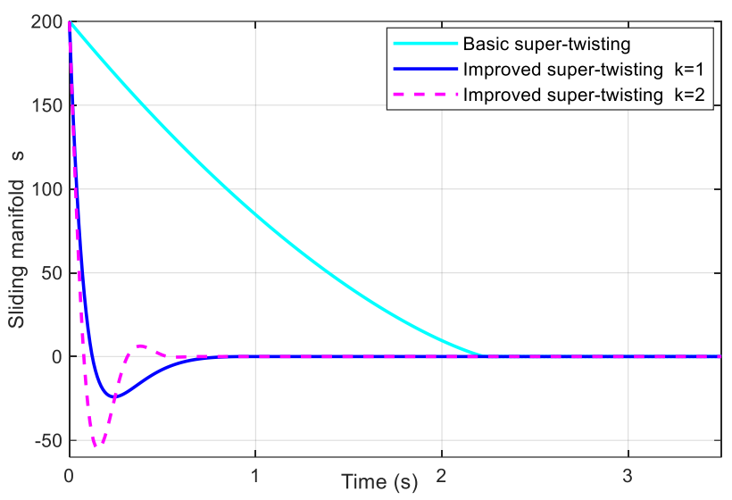
can be gradually reduced from 1 until the system performance begins to decline. The parameter κ is a positive integer. A larger κ can shorten the convergence time of the sliding manifold, but it will lead to the oscillation of the reaching process. It can be seen in Figure 1. The gain parameters of super-twisting sliding mode can be selected according to reference [34], and the upper bound of uncertainty can be determined by experiment. The gain is selected as a 1 = 15 , a 2 = 110 in TDE-STSMC and TDE-FST-FOSMC controllers and a 1 = 1.5 , a 2 = 1.1 is selected in TDE-AFST-FOSMC controllers.
The parameters of the ASMC controller are selected according to reference [16], the parameters are selected as ϖ = 45 , μ 2 = 120 , K K = 20 . Unlike the reference [16], the parameter μ 2 is tuned according to the experimental results. Increasing μ 2 can improve the convergence rate of the estimation, but it will lead to the oscillation of the control voltage, which is very harmful to the motor driver.

4.2. Slalom Path Following

The slalom path following is used to test the steering angle tracking performance of the SBW system. In order to simulate the maneuvering steering in the test, the reference front-wheel steering angle is generated by expression (40):
θ f w = 0.4 s i n ( 0.4 π t )
According to the force analysis of the front wheel, the self-aligning torque can be obtained by τ a = F y f t p + t m , and the lateral tire force of the front wheels F y f can be calculated by F y f = C f α f . According to the literature [36], the front wheel sideslip angle α f can be calculated by α f = β + γ l f / V δ f , and the sideslip angle β can be calculated by β = tan 1 tan ( δ f ) l r / ( l r + l f ) . Therefore, according to the 2-DOF vehicle model, the self-aligning torque can be obtained from expression (41) [15,36].
β = tan 1 tan ( δ f ) l r / ( l r + l f ) γ =   β ˙ + C f + C r m V β C f m V δ f C r l r C f l f m V 2 1 1 τ a = C f ( t m + t p ) ( β + γ l f / V δ f )
Since the experiment platform could not drive on the road, a voltage signal is loaded on the steering motor to simulate the self-aligning torque. The voltage signal can be given by expression (42) [14,15,16]. Where k , J e are the same as parameters in Equation (5), g 0 ( x ) is the control matrix in Equation (34), nw is white noise signal. According to the parameters of the experiment platform and reference [14], the parameters of the vehicle model are set as in Table 2.
u τ a = τ a / ( k J e g 0 ( x ) ) + n w
When the adhesion condition switches on different road, the self-aligning torque is influenced by the adhesion and changes abruptly. The rapidly changing self-aligning torque is applied to the system as a disturbance, which has an adverse impact on the tracking control. In order to verify the robustness and tracking accuracy of different algorithm, typical road conditions are adopted according to reference [14] in this experiment. The tires’ cornering stiffness is set as:
C f = C r = 12,000 N / r a d , 0 < t 18.75 s , s n o w y   r o a d C f = C r = 45,000 N / r a d , 18.75 < t 33.75 s , w e t   a s p h a l t   r o a d C f = C r = 80,000 N / r a d , 33.75 < t 60 s , d r y   a s p h a l t   r o a d
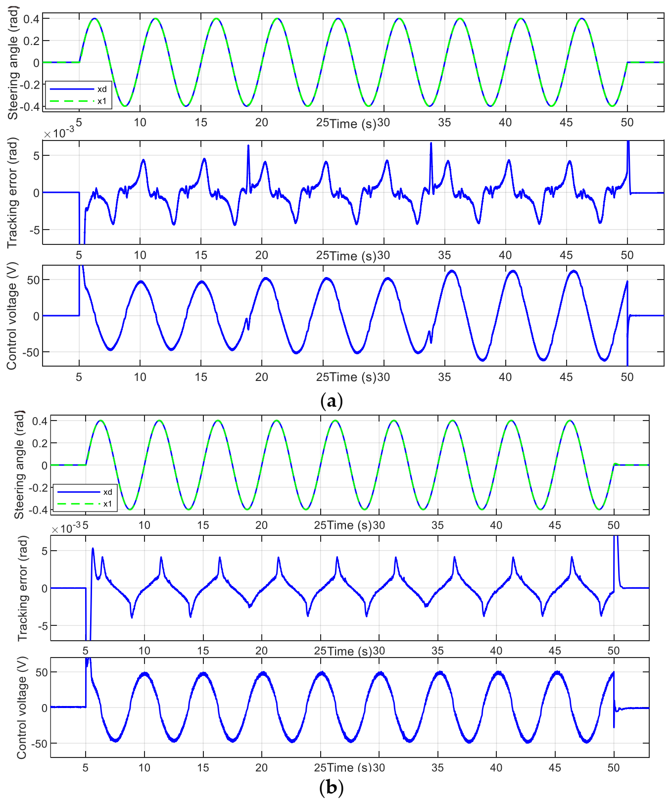
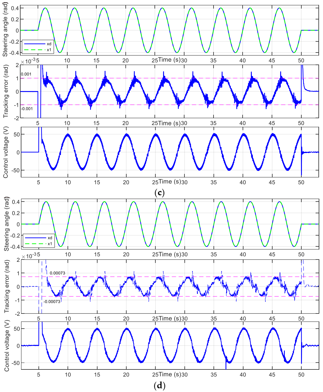
The tracking performance and error comparisons of the different algorithms are shown in Figure 4 and Table 3, respectively. In Figure 4a, corresponding to the ASMC algorithm, at the switching point of different road, the jump of disturbance torque caused a large steering angle tracking error, the amplitude is 0.0067 rad. In the stable stage, the error amplitude is maintained at ± 0.0044 rad. In Figure 4b, corresponding to the TDE-STSMC algorithm, due to the disturbance torque could be estimated and compensated by TDE, there is no large tracking error at the switching point of different road. In the stable stage, the error amplitude is maintained at ± 0.0041 rad. In Figure 4c, corresponding to the TDE-FST-FOSMC algorithm, the tracking error has no obvious change at the switching point of different road. The tracking performance is consistent in three stages. The stable error amplitude is maintained at ± 0.0010 rad. In Figure 4d, corresponding to the TDE-AFST-FOSMC algorithm, the tracking performance is consistent in three stages, there is no obvious change at the switching point of different road. The stable error amplitude is maintained at ± 0.00073 rad. The performance of the TDE-AFST-FOSMC algorithm is the best.
It should be noted that the first derivative of the reference steering angle has a jump at 5 s and 50 s, which is equivalent to introduce an impact in the system. It can be seen from Figure 2 that all the controllers can maintain a stable state, showing good robustness.
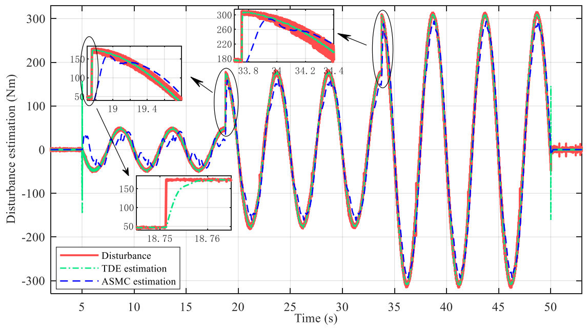
The estimated performance validation results for the perturbations are shown in Figure 5. The self-aligning torque jumps to a large extent when the vehicle turns at the junction of different road surfaces. That is displayed in red lines in the graph as a disturbance. Obviously, the ASMC controller has a large error in estimating disturbance torque. Especially on the snowy road, the ASMC algorithm can only estimate the disturbance torque on the general trend. For TDE, the disturbance term in the original system after a certain small time delay is equivalent to the estimated value of system uncertainty, so the disturbance torque term can be accurately estimated. It can be seen in Figure 5, at the switching point of different road, the self-aligning torque has a jump, and the estimated value of TDE can track the disturbance torque within 7 ms. This shows the good estimation performance of TDE. Therefore, in the case of unknown system model parameters and external disturbances, it has great advantages to apply TDE to closed-loop system control.
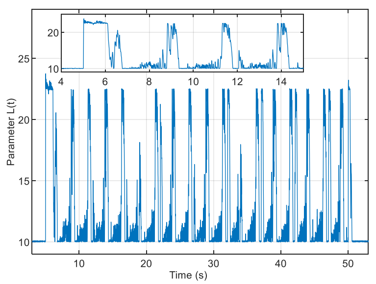
The effect of the adaptive law is shown in Figure 6. It can be seen that L(t) can be adjusted automatically with the change of the system state so that the super-twisting gain parameters a 1 ( t ) , a 2 ( t ) are adjusted accordingly.

4.3. Impact Disturbance Suppression

When a vehicle is driven on a broken road or collides with obstacles, the front wheels will be subjected to a shock torque. Since the mechanical connection between the steering wheel and the front wheels has been removed, the driver cannot exert counter-torque to eliminate the impact. If the SBW system could not quickly estimate the impact torque and suppress it, the vehicle will turn in an unexpected direction and result in a dangerous situation. For this reason, a shock disturbance rejection experiment was carried out to verify the controller’s performance of suppressing impact torque and keeping the direction.
In the experiment, the vehicle is set as running straight on a road with good adhesion conditions. The reference steering angle is set to zero, and the tires cornering stiffness are set as C f = C r = 80,000 N / r a d . A pulse voltage signal with a width of 0.5 s and an equivalent amplitude of 300 Nm is exerted on the steering motor at the 2nd second to simulate the impact disturbance.
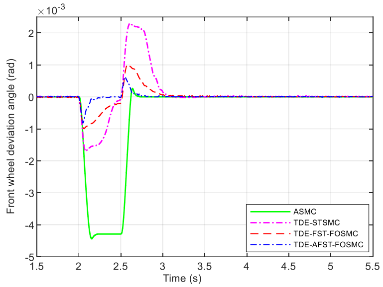
The impact disturbance suppression performance of each algorithm is shown in Figure 7 and Table 4. For the ASMC control, due to the poor disturbance estimation, it results in a front-wheel deflection angle of −0.0044 rad with a duration close to 0.6 s under the impact torque, and the deflection is single direction, which can seriously affect the vehicle safety. For the TDE-AFST-FOSMC, the deflection angle is very small and with a symmetrical shape, and the duration time is very short. It will not cause a dangerous situation.
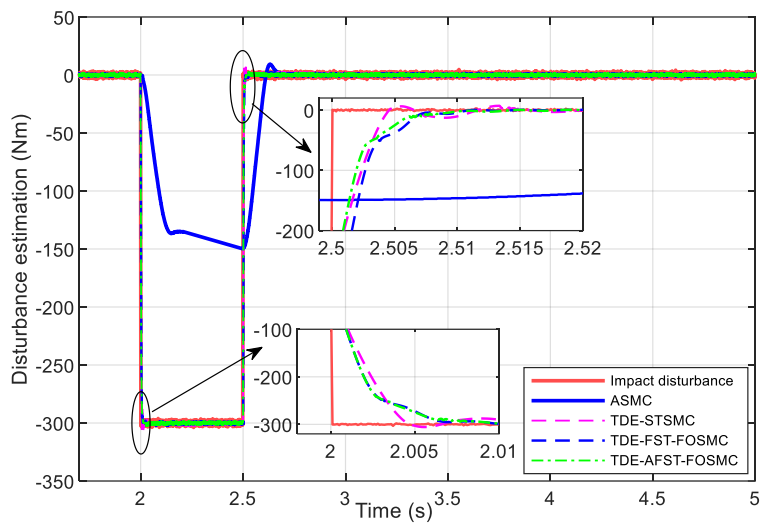
The impact torque estimation performance of each control algorithm is shown in Figure 8. Obviously, the dynamic response of the ASMC algorithm is too slow. The impact torque cannot be accurately estimated. While the TDE adopted by the other three control algorithms can quickly and accurately estimate the impact disturbance torque within 7 ms.

4.4. Double Lane Change Co-Simulation

In this section, CarSim and Simulink co-simulations are conducted on different SBW system controllers to verify the effectiveness of the control algorithm under actual driving conditions. The simulation procedure is selected as “DLC@120 km/h(Quick Start)”, and the “Constant target speed” is modified to 60 km/h. The road friction is selected as “Friction: Mu via S-L Grid”, and the friction coefficient is set as:
{ μ = 0.20 , 0 < S t a t i o n 74 μ = 0.85 , 74 < S t a t i o n 142 μ = 0.20 , 142 < S t a t i o n 210
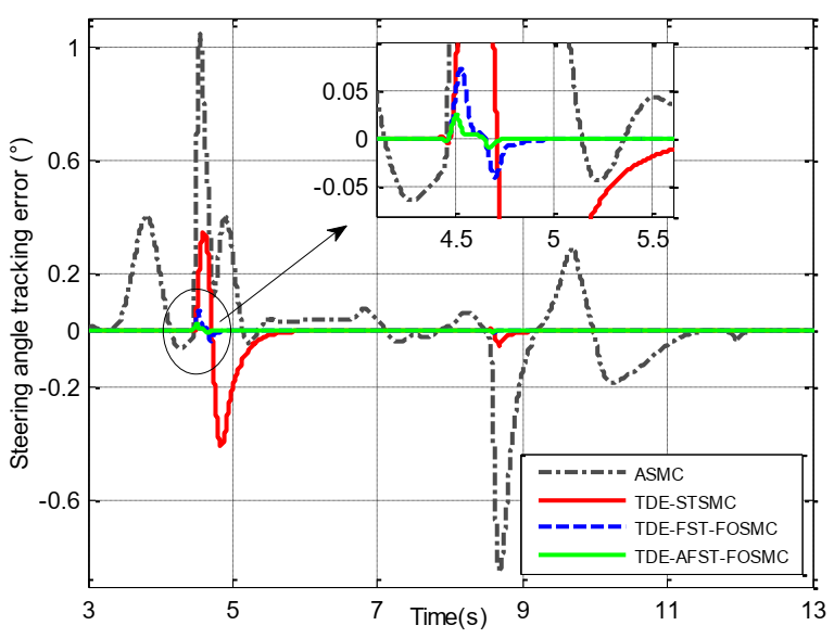
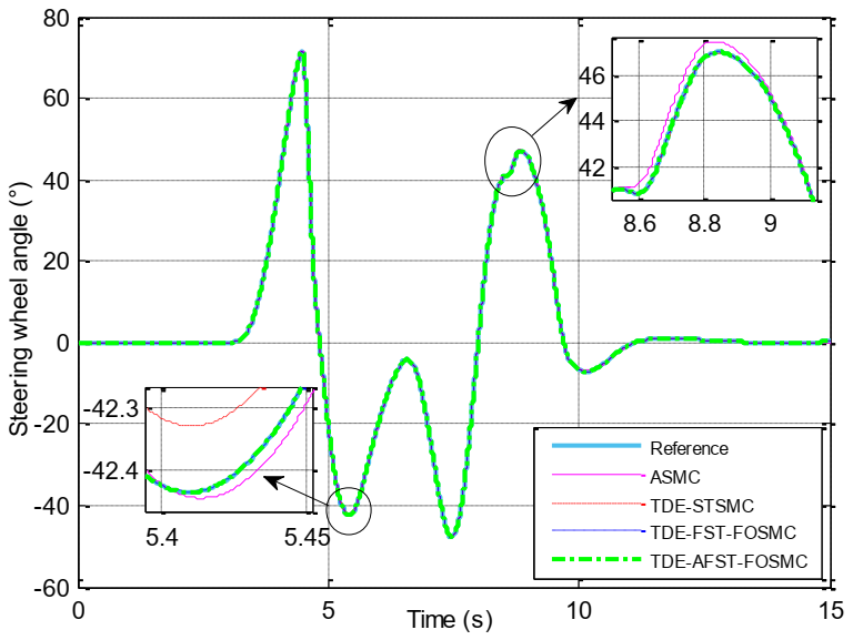
In the DLC simulation test, the “Steer_DM” variable is used as a reference command for the SBW system. The output of the SBW system acts on the vehicle steering system to steer the vehicle. The tracking performance and tracking error in the DLC test are shown in Figure 9; Figure 10 and Table 5. It is obvious that the TDE-AFST-FOSMC algorithm has the best performance when the road adhesion condition changes abruptly, and the maximum tracking errors are +0.024 degrees and −0.01 degrees.
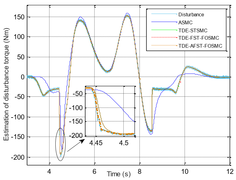
The disturbance estimating performance is shown in Figure 11. The ASMC algorithm has the worst performance. Its dynamic response is severely lagging. The other controllers made a good performance, the TDE estimation can quickly track the disturbance. It is shown in the figure at 4.45 s, the self-aligning torque acquired from CarSim has a large jump due to the road adhesion coefficient change, the TDE estimation can follow the change within 20 ms, and the TDE-AFST-FOSMC controller performs best.
Comparing Figure 10; Figure 11, the ASMC controller produces large steering angle tracking errors at the moments when the disturbance torque estimation error is large. It indicated that the accurate estimation and compensation of the disturbance term can help improve the tracking accuracy. Comparing the tracking performance of TDE-STSMC controller and TDE-FST-FOSMC controller, the maximum tracking error of the former is about 6 times higher than the latter. This shows that the transient response performance of the TDE-FST-FOSMC controller is better due to the fractional-order sliding mode surface and the fast super-twisting structure. Thanks to the adaptive control of the gain parameters, the maximum tracking error of the TDE-AFST-FOSMC controller is reduced to one-third of the TDE-FST-FOSMC controller.

5. Conclusions

In this paper, the time-delay estimation scheme was adopted to solve the problems of precise model design, system parameter determination and estimation of disturbance. An improved super-twisting structure combining with a fractional order sliding mode was proposed to ensure fast dynamical response and high control accuracy. Thanks to the TDE, fast super-twisting with fractional order sliding mode and adaptive algorithm, the proposed control scheme has the advantage of model-free, fast response and high accuracy. Co-simulation and comparative experiments were carried out to validate the effectiveness of the proposed control scheme. Corresponding results indicate that our TDE-AFST-FOSMC can achieve better control performance under practical applications.
However, in the control scheme, the input reference steering angle signal is required to be smooth and second-order differentiable, this puts forward high requirements for the steering angle sensors. Therefore, further research is needed to process the sensor signal, suppress noise interference and improve the reliability of practical application.

Author Contributions

Conceptualization, Y.Y. (Yong Yang) and Y.Y. (Yunbing Yan); Data Curation, Y.Y. (Yong Yang) and X.X.; Writing—Review and Editing, Y.Y. (Yong Yang) and Y.Y. (Yunbing Yan); Supervision, Y.Y. (Yunbing Yan) All authors have read and agreed to the published version of the manuscript.

Funding

This research work was funded by the National Natural Science Foundation of China, grant number 51975428, 51975426; the technological innovation project of Science & Technology Department of Hubei Province, grant number 2018AAA060; the key project of colleges and universities of Henan Province, grant number 19A460027.

Institutional Review Board Statement

Not applicable.

Informed Consent Statement

Not applicable.

Data Availability Statement

The data presented in this study are available on request from the corresponding authors.

Conflicts of Interest

The authors declare no conflict of interest.

References

  1. Zhang, J.; Wang, H.; Zheng, J.C. Adaptive Sliding Mode-Based Lateral Stability Control of Steer-by-Wire Vehicles with Experimental Validations. IEEE Trans. Veh. Technol. 2020, 69, 9589–9600. [Google Scholar] [CrossRef]
  2. Russell, H.E.B.; Gerdes, J.C. Design of variable vehicle handling characteristics using four-wheel steer-by-wire. IEEE Trans. Control Syst. Technol. 2016, 24, 1529–1540. [Google Scholar] [CrossRef]
  3. Hang, P.; Chen, X.; Fang, S.; Luo, F. Robust control for four wheel-independent-steering electric vehicle with steer-by-wire system. Int. J Auto Tech-KOR. 2017, 18, 785–797. [Google Scholar] [CrossRef]
  4. Zhao, W.; Qin, X.; Wang, C. Yaw and lateral stability control for four-wheel steer-by-wire system. IEEE-ASME Trans. Mechatron. 2018, 23, 2628–2637. [Google Scholar] [CrossRef]
  5. Huang, C.; Naghdy, F.; Du, H. Sliding mode predictive tracking control for uncertain steer-by-wire system. Control Eng. Pract. 2019, 85, 194–205. [Google Scholar] [CrossRef]
  6. Zhao, W.; Qin, X. Study on mixed H2/H∞ robust control strategy of four wheel steering system. Sci. China Tech. Sci. 2017, 60, 1831–1840. [Google Scholar] [CrossRef]
  7. Liu, C.; Sun, W.; Zhang, J. Adaptive sliding mode control for 4-wheel SBW system with Ackerman geometry. ISA Trans. 2020, 96, 103–115. [Google Scholar] [CrossRef]
  8. Zhou, W.X.; Wang, Y.Y.; Ahn, C.K.; Cheng, J.; Chen, C.Y. Adaptive Fuzzy Back stepping-Based Formation Control of Unmanned Surface Vehicles With Unknown Model Nonlinearity and Actuator Saturation. IEEE Trans. Veh. Technol. 2020, 69, 14749–14764. [Google Scholar] [CrossRef]
  9. Wang, H.; He, P.; Yu, M. Adaptive neural network sliding mode control for steer-by-wire-based vehicle stability control. J. Intell. Fuzzy Syst. 2016, 31, 885–902. [Google Scholar] [CrossRef]
  10. Wang, H.; Man, Z.; Kong, H. Design and implementation of adaptive terminal sliding-mode control on a steer-by-wire equipped road vehicle. IEEE Trans. Ind. Electron. 2016, 63, 5774–5785. [Google Scholar] [CrossRef]
  11. Sun, Z.; Zheng, J.; Wang, H. Adaptive fast nonsingular terminal sliding mode control for a vehicle steer-by-wire system. IET Control Theory Appl. 2017, 11, 1245–1254. [Google Scholar] [CrossRef]
  12. Iqbal, J.; Zuhaib, K.M.; Han, C. Adaptive global fast sliding mode control for steer-by-wire system road vehicles. Appl. Sci. 2017, 7, 738. [Google Scholar] [CrossRef]
  13. Ye, M.; Wang, H. Robust adaptive integral terminal sliding mode control for steer-by-wire systems based on extreme learning machine. Comput. Electr. Eng. 2020, 86, 106756. [Google Scholar] [CrossRef]
  14. Sun, Z.; Zheng, J.C.; Man, Z.H.; Fu, M.Y.; Lu, R.Q. Nested adaptive super-twisting sliding mode control design for a vehicle steer-by-wire system. Mech. Syst. Signal Process. 2019, 122, 658–672. [Google Scholar] [CrossRef]
  15. Yang, Y.; Yan, Y.; Xu, X.; Gong, B. Super-twisting algorithm with fast super-twisting disturbance observer for steer-by-wire vehicles. Proc. IMechE Part D J. Auto. Eng. 2021, 235, 2324–2340. [Google Scholar] [CrossRef]
  16. Sun, Z.; Zheng, J.; Man, Z. Robust control of a vehicle steer-by-wire system using adaptive sliding mode. IEEE Trans. Ind. Electron. 2016, 63, 2251–2262. [Google Scholar] [CrossRef]
  17. Bresch-Pietri, D.; Chauvin, J.; Petit, N. Adaptive backstepping controller for uncertain systems with unknown input time-delay. Application to SI engines. In Proceedings of the 49th IEEE Conference on Decision and Control (CDC), Atlanta, GA, USA, 15–17 December 2010; pp. 3680–3687. [Google Scholar]
  18. Bresch-Pietri, D.; Chauvin, J.; Petit, N. Adaptive control scheme for uncertain time-delay systems. Automatica 2012, 48, 1536–1552. [Google Scholar] [CrossRef]
  19. Bresch-Pietri, D.; Krstic, M. Delay-adaptive control for nonlinear systems. IEEE Trans. Automat. Contr. 2014, 59, 1203–1218. [Google Scholar] [CrossRef]
  20. Youcef-Toumi, K.; Ito, O. A time delay controller design for systems with unknown dynamics. ASME J. Dyn. Syst. Meas. Control. 1990, 112, 133–142. [Google Scholar] [CrossRef]
  21. Hsia, T.C. A new technique for robust control of servo systems. IEEE Trans. Ind. Electron. 1989, 36, 1–7. [Google Scholar] [CrossRef]
  22. Wang, Y.; Gu, L.; Chen, B.; Wu, H. A new discrete time delay control of hydraulic manipulators. Proc. IMechE Part I J. Syst. Control Eng. 2017, 231, 168–177. [Google Scholar] [CrossRef]
  23. Wang, Y.; Yan, F.; Chen, J. A new adaptive time-delay control scheme for cable-driven manipulators. IEEE Trans. Ind. Informat. 2019, 15, 3469–3481. [Google Scholar] [CrossRef]
  24. Lee, J.; Chang, P.H.; Jin, M. Adaptive integral sliding mode control with time-delay estimation for robot manipulators. IEEE Trans. Ind. Electron. 2017, 64, 6796–6804. [Google Scholar] [CrossRef]
  25. Wang, Y.Y.; Li, S.Z.; Wang, D.; Ju, F.; Chen, B.; Wu, H.T. Adaptive Time-Delay Control for Cable-Driven Manipulators with Enhanced Nonsingular Fast Terminal Sliding Mode. IEEE Trans. Ind. Electron. 2021, 68, 2356–2367. [Google Scholar] [CrossRef]
  26. Van, M.; Ge, S.S.; Ren, H.L. Finite Time Fault Tolerant Control for Robot Manipulators Using Time Delay Estimation and Continuous Nonsingular Fast Terminal Sliding Mode Control. IEEE Trans. Cybern. 2017, 47, 1681–1693. [Google Scholar] [CrossRef] [PubMed]
  27. Baek, J.; Jin, M.; Han, S. A New Adaptive Sliding-Mode Control Scheme for Application to Robot Manipulators. IEEE Trans. Ind. Electron. 2016, 63, 3628–3637. [Google Scholar] [CrossRef]
  28. Kali, Y.; Saad, M.; Benjelloun, K.; Khairallah, C. Super-twisting algorithm with time delay estimation for uncertain robot manipulators. Nonlinear Dyn. 2018, 93, 557–569. [Google Scholar] [CrossRef]
  29. Wang, Y.; Chen, J.; Yan, F. Adaptive super-twisting fractional-order nonsingular terminal sliding mode control of cable-driven manipulators. ISA Trans. 2019, 86, 163–180. [Google Scholar] [CrossRef]
  30. Wang, Y.; Li, B.; Yan, F. Practical adaptive fractional-order nonsingular terminal sliding mode control for a cable-driven manipulator. Int. J. Robust Nonlinear Control. 2019, 29, 1396–1417. [Google Scholar] [CrossRef]
  31. Wang, Y.; Yan, F.; Zhu, K. A new practical robust control of cable-driven manipulators using time-delay estimation. Int. J. Robust Nonlinear Control. 2019, 29, 3405–3425. [Google Scholar] [CrossRef]
  32. Wang, Y.; Zhu, K.; Yan, F. Adaptive super-twisting nonsingular fast terminal sliding mode control for cable-driven manipulators using time-delay estimation. Adv. Eng. Softw. 2019, 128, 113–124. [Google Scholar] [CrossRef]
  33. Kilbas, A.A.; Srivastava, H.M.; Trujillo, J.J. Fractional integrals and fractional derivatives. In Theory and Applications of Fractional Differential Equations, 1st ed.; Elsevier: Amsterdam, The Netherlands, 2006; pp. 69–133. [Google Scholar]
  34. Edwards, C.; Shtessel, Y. Adaptive dual-layer super-twisting control and observation. Int. J. Control. 2016, 89, 1759–1766. [Google Scholar] [CrossRef] [Green Version]
  35. Lu, K.; Xia, Y.; Zhu, Z. Sliding mode attitude tracking of rigid spacecraft with disturbances. J. Frankl. Inst. 2012, 349, 413–440. [Google Scholar] [CrossRef]
  36. Rajamani, R. Lateral vehicle dynamics. In Vehicle Dynamics and Control; Rajamani, R., Boston, M.A., Eds.; Springer: Berlin/Heidelberg, Germany, 2012; pp. 20–24. [Google Scholar]
Figure 1. Convergence time comparison of different super-twisting structures.
Electronics 10 02424 g001
Figure 2. Block diagram of TDE-based AFST-FOSMC control scheme.
Electronics 10 02424 g002
Figure 3. Experimental platform of the SBW system.
Electronics 10 02424 g003
Figure 4. Tracking performance and the control voltage: (a) ASMC algorithm; (b) TDE-STSMC algorithm; (c) TDE-FST-FOSMC algorithm; (d) TDE-AFST-FOSMC algorithm.
Electronics 10 02424 g004aElectronics 10 02424 g004b
Figure 5. Estimation of disturbance torque in slalom path following.
Electronics 10 02424 g005
Figure 6. Adaptive effect of control parameter L(t).
Electronics 10 02424 g006
Figure 7. Front wheel deviation under shock disturbance.
Electronics 10 02424 g007
Figure 8. Performance of estimation of shock disturbance torque.
Electronics 10 02424 g008
Figure 9. Tracking performance of steering wheel angle.
Electronics 10 02424 g009
Figure 10. Tracking error of steering wheel angle.
Electronics 10 02424 g010
Figure 11. Estimation performance of disturbance torque.
Electronics 10 02424 g011
Table 1. SBW system parameters.
ParametersValue
Back EMF coefficient ke0.2209 V·s/rad
Torque coefficient km0.3255 Nm/A
Motor resistance R2.083 Ω
Equivalent moment of inertia Jeq0.0010 kg·m2
Equivalent viscous resistance coefficient Beq0.0090 Nm·s/rad
Coulomb friction moment τ F C 8.0 Nm
Steering gear ratio k118
Steering motor reduction ratio k220.5
Table 2. Vehicle model parameters.
ParametersValue
Mass of vehicle m1170 kg
Vehicle speed V15 m/s
The distances of front axle from the c.g. of the vehicle lf0.96 m
The distances of rear axle from the c.g. of the vehicle lr0.84 m
Front-wheel mechanical trail tm0.023 m
Front-wheel pneumatic trail tp0.015 m
Table 3. Tracking errors comparison of different algorithms in slalom path following.
ControllerASMCTDE-STSMCTDE-FST-FOSMCTDE-AFST-FOSMC
Maximum error
(rad)
0.00670.00410.0015+0.0011
Steady-stat error
(rad)
±0.0044±0.0041±0.0010±0.00073
Table 4. Deviation of the front wheels under shock disturbance.
ControllerASMCTDE-STSMCTDE-FST-FOSMCTDE-AFST-FOSMC
Deviation angle
(rad)
0+0.0023+0.001+0.0006
−0.0044−0.0017−0.001−0.0008
Table 5. Steering wheel angle tracking errors of controllers in the DLC test.
ControllerASMCTDE-STSMCTDE-FST-FOSMCTDE-AFST-FOSMC
Tracking error+1.044+0.344+0.073+0.024
−0.85−0.41−0.04−0.01
Publisher’s Note: MDPI stays neutral with regard to jurisdictional claims in published maps and institutional affiliations.

