6D Pose Estimation for Subsea Intervention in Turbid Waters

Abstract

Manipulation tasks on subsea instalments require extremely precise detection and localization of objects of interest. This problem is referred to as “pose estimation”. In this work, we present a framework for detecting and predicting 6DoF pose for relevant objects (fish-tail, gauges, and valves) on a subsea panel under varying water turbidity. A deep learning model that takes 3D vision data as an input is developed, providing a more robust 6D pose estimate. Compared to the 2D vision deep learning model, the proposed method reduces rotation and translation prediction error by ($-\Delta {0.39}^{\circ }$) and translation ($-\Delta 6.5$ mm), respectively, in high turbid waters. The proposed approach is able to provide object detection as well as 6D pose estimation with an average precision of 91%. The 6D pose estimation results show ${2.59}^{\circ }$ and $6.49$ cm total average deviation in rotation and translation as compared to the ground truth data on varying unseen turbidity levels. Furthermore, our approach runs at over 16 frames per second and does not require pose refinement steps. Finally, to facilitate the training of such model we also collected and automatically annotated a new underwater 6D pose estimation dataset spanning seven levels of turbidity.

1. Introduction

Autonomy underwater has until recently been limited to use-cases where localization and navigation can be based on sensors which exhibit positional drifts such as Doppler Velocity Logs (DVLs), compasses and IMUs. Such inaccurate localization methods are not suitable for intervention, inspection and maintenance use-cases where accurate localization is key. Underwater optical (3D) imaging has opened up possibilities for providing high-density information of the AUV surroundings, which is an enabler for accurate detection and 6DoF localization of objects. 6DoF localization refers to estimating a transformation that maps an object from object to camera coordinate system (three degrees for translation and rotation). In terrestrial applications, deep learning on 3D images has revolutionized detection and localization [1]. However, its application and performance for object detection and localization on underwater imagery has not been explored to the same degree. In this paper, we propose a deep learning based network for 6DoF localization of known objects using underwater 3D range-gated images.

There are a range of 2D and 3D vision systems that can be used to solve a wide range of applications on ROVs and AUVs. However, water turbidity, absorption and scattering or colour distortion often limits the use of standard 2D and 3D vision systems as a solution to the problem of vision-based subsea object detection and pose estimation. 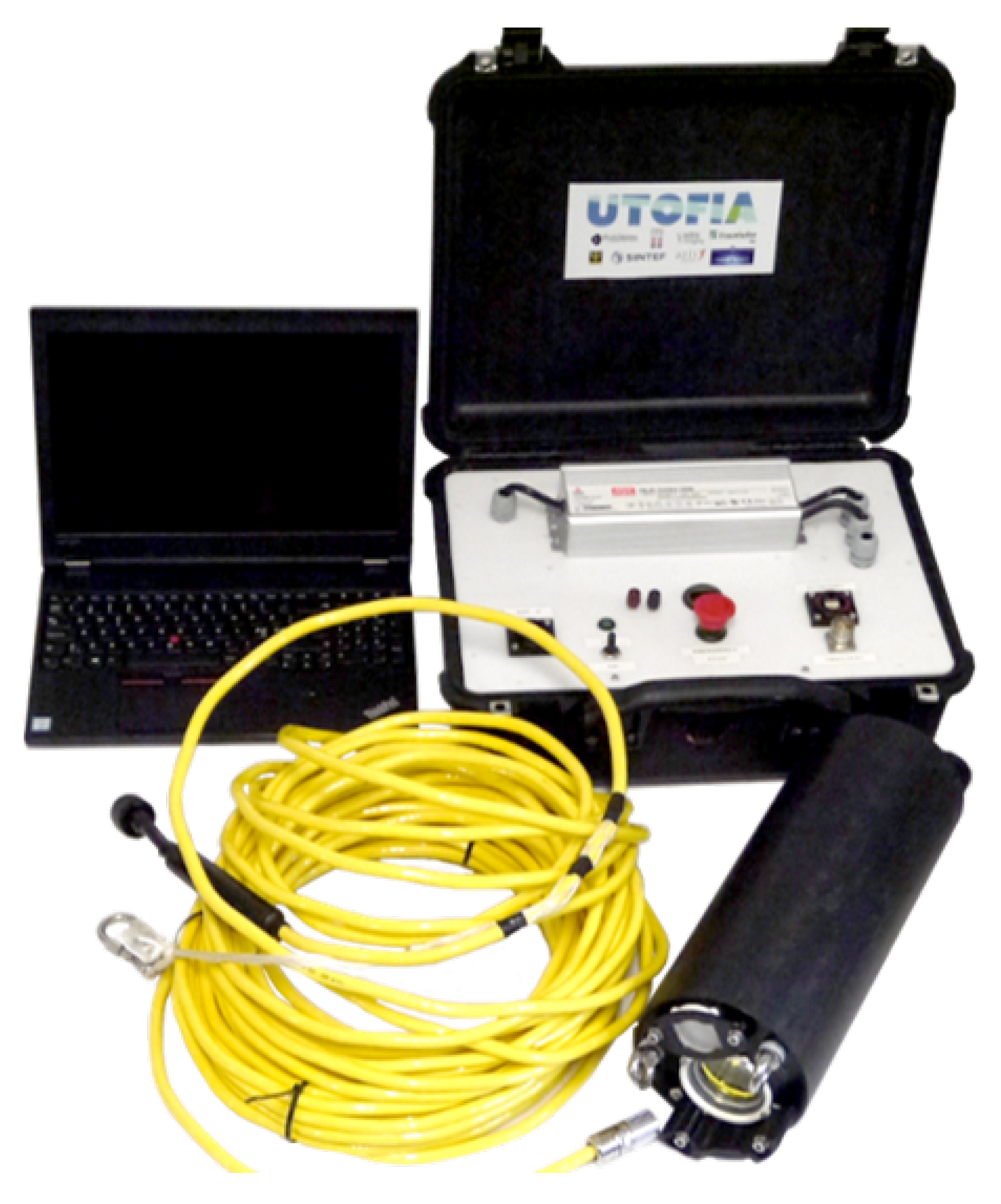Numerous optical 3D vision systems have been proposed for the purpose of subsea object detection, such as structured light and stereo-vision [2]. Stereo-vision has the advantage of being a relatively simple and cost-effective approach for underwater 3D object detection. However, such approaches tend to struggle with limited viewing distance and water turbidity, which smear out the image details that are used for object detection and pose estimation. To improve the chances of detecting subsea objects and estimate object pose more precisely, this paper proposes to equip ROVs and AUV with a range-gated 3D camera (Utofia), which is described in detail in [3]. The advantage of the 3D range-gated camera is the combination of depth resolution, field of view, real-time 3D acquisition (10 Hz), and its resistance to turbidity makes it ideal for real-time subsea object detection, localization and pose estimation.

From an algorithmic perspective, 3D vision-based pose estimation approaches focus on matching an extracted region of interest in an image or point cloud with a template CAD model to estimate the 6D pose [4]. Although such approaches achieve good 6D pose estimation accuracy, the computational complexity increases linearly with the number of objects. Furthermore, they require an object segmentation algorithm for cropping object of interest as a pre-processing step and compute 6D pose for each object individually. Therefore, such approaches are not well suited for multi-object 6D pose estimation due to runtime limitations. In this paper, we propose a deep learning model that takes 3D data which does not encounter these issues. The proposed deep learning model is able to detect and estimate 6D-pose estimation under different turbidity in an end-to-end fashion using 3D data.

Next, we review existing methods related to the topic of deep learning for object detection and pose estimation for 3D data. Our review here is intended to highlight the broad approaches of existing 6D pose estimation algorithms for underwater and terrestrial applications, and to provide appropriate background for our work.

Terrestrial 6D pose estimation: Based on the sensor, 6D pose estimation can be roughly divided into two groups: 2D vision and 3D vision based 6D pose estimation. 2D vision based approaches rely on 2D image data to predict 6D pose. PoseCNN [5] proposes a two stage process. The first stage extracts feature maps with different resolutions from the input image. This stage is the backbone of the network since the extracted features are shared across all the tasks performed by the network. The second stage consists of embedding the high-dimensional feature maps generated by the first stage into low-dimensional, task specific features. Then, the network performs three different tasks that lead to the 6D pose estimation, i.e., semantic labelling, 3D translation estimation, and 3D rotation. Using iterative closest point(ICP) as a refinement phase PoseCNN makes their 6D pose estimation accurate. In [6], a method named CosyPose was proposed, which uses multiple views to reconstruct a scene composed of multiple objects to estimate 6D pose in three stages. In the first stage, for each view, initial object candidates are estimated separately. In the second stage, the object candidates are matched across views to recover a single consistent scene. In the third stage, object pose hypotheses across different views are jointly refined to minimize multi-view reprojection error. Bukschat et al. [7] proposed a single stage approach, EfficientPose architecture that extends EfficientDet [8] for 6D pose estimation by adding translation and iterative refining rotation subnetworks. In general, 2D vision based approaches are less robust for 6D pose estimation due to geometric information are partly lost due to projection, and different keypoints in 3D space may be overlapped and hard to be distinguished after projection to 2D space. On the other hand, 3D vision based approaches work on RGBD or point cloud data. Wang et al. proposed [9] a DenseFusion method for 6D pose estimation. DenseFusion first performs image segmentation of object of interest and computes 6D pose in two stage process. In the first stage, image and geometric features are extracted by passing through a two stream network using cropped image data and point cloud, respectively. In the second stage, the RGB colours and point cloud from the depth map are encoded into embedding and fused at each corresponding pixel. The pose predictor produces a pose estimate for each pixel and the predictions are voted to generate the final 6D pose prediction of the object. In addition, it finally refines the result in an iterative procedure. In [10], PVN3D is proposed which also has a two-stage pipeline. PVN3D extends a 2D key points to 3D key points detection followed by a pose parameters fitting module. They used a least-square fitting algorithm to the predicted keypoints to estimate 6DoF pose parameters.

Underwater 6D pose estimation: The results of previous object pose estimation mostly focus on terrestrial environments and optical vision based 6D pose estimation has not been widely used in underwater scenarios. In [11], to deal with lack of underwater dataset, they generated a synthetic underwater dataset for pose estimation and object detection task. The pose estimation is done in two stages. Firstly, Mask R-CNN [12] is used to detect object of interest. Secondly, the cropped object is passed through a second network for pose estimation using Euler angle representation. Miguel et al. [13] proposed to use PointNet [14] to recognize pipes and valves in 3D RGB point cloud information provided by a stereo camera. However, the authors do not consider realistic cases such as water turbidity. In Nielsen et al. [15], a PoseNet architecture [16], which regresses both position and orientation simultaneously, is explored for underwater application. Their approach takes RGB image as input and considers a single turbidity and a single object subsea connector that is connected to a metal stick.

In contrast to earlier works, the proposed model is a single stage network for fast and efficient underwater object detection and 6D pose estimation using 3D data. Furthermore, the proposed model is able to estimate 6D pose under seven different turbidity levels with 91.03% mAP and average pose deviation of 2.59${}^{\circ }$. To summarize, the main contributions of this work are as follows:

• The use of 3D range-gated camera for underwater 6D for efficient pose estimation.
• A single stage end-to-end sub-sea object detection and 6D pose estimation deep learning model that runs 16 frames per second with 91.03% mAP and average deviation in rotation (2.59${}^{\circ }$), and translation ($6.49$ cm) as compared to the ground truth data over test turbidities.
• Ground truth data generation setup for efficient data collection for training deep learning models and a labelled dataset containing six underwater objects such as valves, fish-tails etc. with a total of 30 K frames.

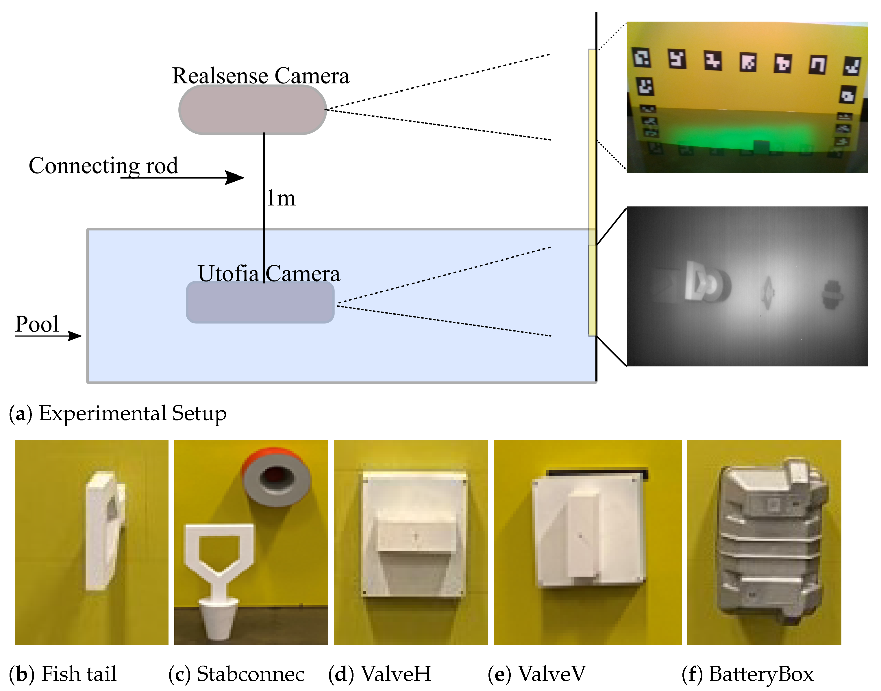
This paper is structured as follows. Section 2 describes experimental setup for data acquisition and automated data labelling procedure. Section 3 describes the study methodology to estimate object pose using 3D vision data. Section 4 presents and analyses the results with discussion on dataset bias analysis.

2. Data Acquisition and Pre-Processing

There are few, if any, relevant datasets pertaining to 6DoF localization underwater at different turbidities. One of the main contributions of this paper is the approach for gathering an underwater 3D dataset of relevant objects for the subsea-industry, where the ground truth 6DoF pose of the objects is automatically generated, even under turbid conditions.

2.1. Data Acquisition Setup

Figure 1 shows the mockup subsea panel we created, which includes valves, stab-connector, gauges and fish-tails. These objects are placed at known locations on a 3 m × 2 m flat plate.

Fifteen Aruco markers [17] are printed at known locations along the border of the plate. If one or more of the Aruco markers are observed by a camera, they can be used to establish the pose of the objects. The plate is placed at the end of a 4 m × 8 m pool with a depth of 1.5 m. Hence, the top row of Aruco markers will be located above water, while the objects and the lower 4 Aruco markers will be located under water. The Aruco markers located underwater will at high turbidities be difficult to locate precisely. Consequently, we rigidly attach a 2D camera to the Utofia camera housing as shown in Figure 1a, such that the 2D camera is located above water and will always have a clear view of the markers above water. We calibrated the extrinsic camera parameters of the above water camera in relation to the Utofia camera by comparing detections of the markers above water with detections from the Utofia camera under water in clear water. They do not image the same markers, but we exploit the fact that we know the relative positioning of the different markers on the board to solve for the extrinsics. The intrinsic parameters where established using standard checker board camera calibration [18,19].

Turbidity was increased in the pool by adding blue modelling clay dissolved in water. At each turbidity level, we measured the attenuation length of the water—i.e., the length at which $1/e\approx 37\%$ amount of light remains. We acquired datasets of the subsea panel at 7 different turbidities ranging from 8.3 m attenuation length down to 2.2 m attenuation length. Each turbidity specific dataset was acquired by continuously capturing images from the two cameras while moving the camera rig such that the objects were imaged with a wide variety of viewpoints and distances. The sub-sea panel and sample frames with the ground truth pose is shown in Figure 1 and Figure 2, respectively.

2.2. A Range-Gated Underwater 3D Camera

Capturing high quality underwater (3D) imagery is challenging due to poor visibility underwater and technological limitations in sensor design. Recently, the range gating 3D system Utofia [3] as shown in Figure 3, has provided an opportunity to capture high-resolution underwater intensity and depth images. We include a short description here for completeness.

The Utofia camera is equipped with a 532 nm 3.5 mJ laser which produces short pulses (1ns width). The combination of the short pulsed laser with a megapixel camera with a fast shutter allows us to produce range-gated images at 1000 Hz. An FPGA sequencer is implemented on the camera, which includes functionality for real-time acquisition of range-gated sweeps, where the minimal distance between two ranges is an increase of 1.67 ns (18.8 cm) between the firing of the laser pulse and the opening of the shutter. The FPGA also includes a super-resolved 3D algorithm which estimates the pixel-wise depth down to 1cm, depending on the signal to noise (SNR) ratio.

3. Methods

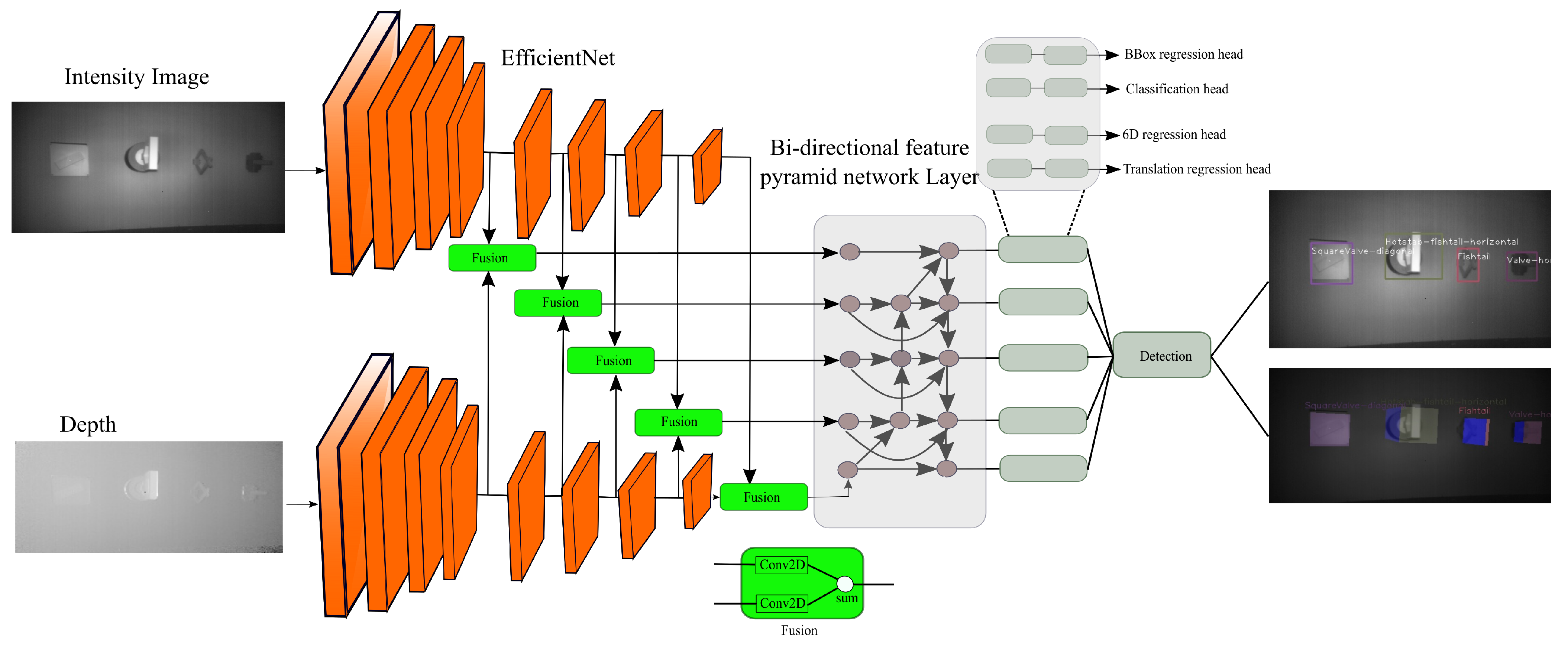
The proposed pipeline shown in (Figure 4) is divided into 4 sub-tasks that combined can solve the task of object 6D pose estimation. Class and box prediction sub-networks handle detecting objects with 3D data while handling multiple object categories and instances. The class and box prediction sub-networks follow EfficientDet architecture [8] using the EfficientNet base network [20]. Rotation and translation prediction sub-networks estimate the rigid transformation (3D rotation $R\in SO(3)$ and a translation $t\in {\mathbb{R}}^3$) that transforms an object from a world coordinate system to the camera world coordinate system. The features from intensity and depth network stream are merged and passed to a bidirectional feature pyramid network layer (BiFPN) [8]. BiFPN leveraged a convolutional neural network (CNN) to extract bidirectional feature maps at different resolutions.

3.1. Rotation Sub-Network

The rotation sub-network takes in BiFPN feature maps and predicts a rotation vector in a continuous 6D representation [21], which has been shown to lead to a more stable CNN training than quaternions. The sub-network architecture is similar to class and box prediction sub-networks, except that sigmoid activation is replaced with SiLU activation function [22], which provides a better gradient flow. The last conv layer of rotation sub-network have dimension of $6\times N_c$, where $N_c$ is the number of anchor boxes. The orthogonal properties of rotation matrices are enforced by the network by using the Gram–Schmidt orthogonalization procedure Equation (1). Given the rotation sub-network outputs $(\overrightarrow{\mathbf{u}},\overrightarrow{\mathbf{v}})\in {\mathbb{R}}^3$ the 3D rotation matrix is reconstructed as $R\in SO(3)$ as follows:

$$\begin{array}{c}\hfill \begin{array}{cc}\hfill {\overrightarrow{\mathbf{r}}}_1& =\frac{\overrightarrow{\mathbf{u}}}{\parallel \overrightarrow{\mathbf{u}}\parallel },\hfill \\ \hfill \overrightarrow{{\mathbf{r}}_2}& =\frac{\overrightarrow{\mathbf{q}}}{\parallel \overrightarrow{\mathbf{q}}\parallel },\overrightarrow{\mathbf{q}}=\overrightarrow{\mathbf{v}}-(\overrightarrow{{\mathbf{r}}_1}·\overrightarrow{\mathbf{v}})\overrightarrow{{\mathbf{r}}_1}\hfill \\ \hfill \mathbf{R}& =(\overrightarrow{{\mathbf{r}}_1}\overrightarrow{{\mathbf{r}}_2}(\overrightarrow{{\mathbf{r}}_1}\times \overrightarrow{{\mathbf{r}}_2}))\hfill \end{array}\end{array}$$

(1)

3.2. Translation Sub-Network

The network architecture for the translation sub-network follows similar architecture as the rotation sub-network and predicts the 3D translation vector $\mathbf{T}=(t_x,t_y,t_z)$ such that $\mathbf{T}$ is the coordinate of the object origin in the camera coordinate system. Rather than regressing the $\mathbf{t}$ directly, the sub-network estimates the centre pixel coordinate offset from the anchor box centre and the normalized distance $t_{nz}=\frac{t_z}{t_{zmax}}$. This reformulation has been shown to make bounding box regression task easier to learn [23]. The centre pixels, $\mathbf{c}=(c_x,c_y)$ is the centre of the projected 3D object on image coordinate [5]. Given the sub-network estimate for $\mathbf{c}$ in the image, the normalized distance $t_{nz}$ and the camera intrinsic parameters, the 3D translation vector $\mathbf{T}=(t_x,t_y,t_z)$ can be recovered following the perspective camera model as:

$$\begin{array}{c}\hfill \begin{array}{cc}\hfill t_z& =t_{nz}{t}_{zmax}\hfill \\ \hfill t_x& =\frac{t_z(c_x-p_x)}{f_x},\hfill \\ \hfill t_y& =\frac{t_z(c_y-p_y)}{f_y},\hfill \end{array}\end{array}$$

(2)

with the 2D projection of centre of the 3D object $\mathbf{c}=(c_x,c_y)$, focal lengths of the camera $f_x,f_y$ and principal point $(c_x,c_y)$. Here, the principal point is the point where the optical axis intersects the image plane.

3.3. Loss

To regress the 6D pose, we use Equation (3) as a loss function during the training. This loss function is similar to that of DenseFusion and EfficientPose [7,9], except that loss is computed for the 3D bounding box coordinates:

$${\mathcal{L}}_p=\frac{1}{m}\sum _{i=0}^m{∥\left(\tilde{\mathbf{R}}{\mathbf{p}}_{\mathrm{i}}+\tilde{\mathbf{T}}\right)-\left(\mathbf{R}{\mathbf{p}}_{\mathrm{i}}+\mathbf{T}\right)∥}^2$$

(3)

where, ${\mathbf{p}}_{\mathrm{i}}$ denotes the ith corner of the 3D bounding box points from the objects 3D model, $\left[\tilde{\mathbf{R}}\right|\tilde{\mathbf{T}}]$ is the ground truth pose, where $\tilde{\mathbf{R}}$ is the rotation matrix of the object and $\tilde{\mathbf{T}}$ is the translation. Furthermore, to handle symmetric objects in the rotation sub-network we used PoseLoss [5], which measures the average squared distance between points on the correct model pose:

$${\mathcal{L}}_r=\frac{1}{m}\sum _{i=0}^m{∥\tilde{\mathbf{R}}{\mathbf{p}}_{\mathbf{i}}-\mathbf{R}{\mathbf{p}}_{\mathbf{i}}∥}^2$$

(4)

the complete transformation loss function ${\mathcal{L}}_{trans}$ is given by:

$${\mathcal{L}}_{trans}={\mathcal{L}}_r+{\mathcal{L}}_p$$

(5)

3.4. Data Pre-Processing and Training

The dataset is divided into a training and test set; the training set contains all $\approx 18$ K images from turbidity 0, 2, 4, 5, and 7, while $\approx 12$ K images from turbidity 1, 3, and 6 is used for the test set. Our capturing setup configuration is stationary such that orientation of objects, ordering of objects, positioning is the same. This could result in the learning algorithm to memorize the configuration rather than learning the actual pose leading to overfitting the training data. To circumvent this problem we have introduced pre-processing step and random augmentation. First, the depth image is smoothed with median filter of size (5, 5) as a pre-processing step to improve object detection. Both intensity and depth image values are normalized between 0 and 1. Second, ground truth rotation matrix is augmented by applying random rotation (0${}^{\circ }$ to 360${}^{\circ }$) and scale (0.7 to 1.3). Random noise is added for objects that lie on the image boundary or partially visible after augmentation with a probability of 0.5. Finally, the intensity and depth images are resized to ($480\times 256$) and padded with zeros to a fixed size of ($512\times 512$).

We trained the network for 100 epochs, using mini-batches of 16 images, and observed that the loss converged after approximately 50 epochs. The network outputs four parameters for each object and the final loss function has the following form.

$${\mathcal{L}}_T=\beta {\mathcal{L}}_{class}+\tau {\mathcal{L}}_{reg}+\eta {\mathcal{L}}_{trans}$$

(6)

For all of our experiments we set $\beta =1,\tau =1$ and $\eta =0.5$. These values were found empirically. The first term is classification (focal) loss and we used $\alpha =0.25$ and $\gamma =2.0$, while the second term is the bounding box regression loss. The last term is the transformation loss Equation (6).

4. Results and Discussions

The performance of the network under different turbidities is evaluated based on the Relative Translation Error (RTE) and Relative Rotation Error (RRE) metrics that measures the deviations between the predicted and and ground truth pose as defined in [24]. Furthermore, mean Average Precision [25] (mAP) is computed by taking the average of precision over all the objects at 0.5 IoU (Intersection over union). Given the ground truth rotation $\mathbf{R}$ and translation $\mathbf{T}$ of each object, the RTE and RRE are defined as follows:

$$\begin{array}{c}\hfill \begin{array}{cc}\hfill RTE& =\parallel \tilde{\mathbf{T}}-\mathbf{T}\parallel \hfill \\ \hfill RRE& =arccos(\frac{trace({\tilde{\mathbf{R}}}^{\mathbf{T}}\mathbf{R})-1}{2})\hfill \end{array}\end{array}$$

(7)

where $\tilde{\mathbf{T}}$ and $\tilde{\mathbf{R}}$ denote the estimated translation vector and translation matrix, respectively.

Table 1. 6D pose and 2D object detection performance. The 2D object detection (2D OD) is measured in average precision (AP). The translation and rotation errors (RTE, RRE) are represented in cm and degree (${}^{\circ }$), respectively.

Turbidity	Metric	Avg	Fish-Tail	Square-Valve-Vertical	Fish-Tail-Hotstab	Square-Valve-Horizontal	Battery-Box
Turbidity1	2D OD	0.91	0.89	0.91	0.89	0.93	0.95
	$T_{err}$	6.54	8.78	5.87	5.41	5.72	6.92
	$R_{err}$	2.62	2.19	3.05	2.43	2.72	2.69
Turbidity3	2D OD	0.91	0.92	0.90	0.89	0.88	0.98
	$T_{err}$	6.61	8.58	5.52	5.40	6.07	7.49
	$R_{err}$	2.56	2.27	2.85	2.44	2.69	2.58
Turbidity6	2D OD	0.91	0.90	0.91	0.87	0.87	0.97
	$T_{err}$	6.33	7.89	5.48	5.37	5.92	6.97
	$R_{err}$	2.59	2.29	2.87	2.46	2.80	2.52
Overall	2D OD	0.91	0.90	0.91	0.89	0.90	0.96
	$T_{err}$	6.49	8.41	5.62	5.39	5.90	7.12
	$R_{err}$	2.59	2.25	2.92	2.44	2.74	2.60

lists the AP, RTE, RRE of the proposed model for the turbidities in the test dataset. Looking at the metrics presented for each class, the level of difficulty for object detection and pose estimation underwater varies with turbidity and the size of object of interest. It is important to note that most of the objects considered in our experiment are symmetric which is known to be more challenging than non-symmetric objects [16]. Overall, the proposed method is able to localize and estimate objects with 6D poses in a single shot without the need of further post-processing or refinement step. 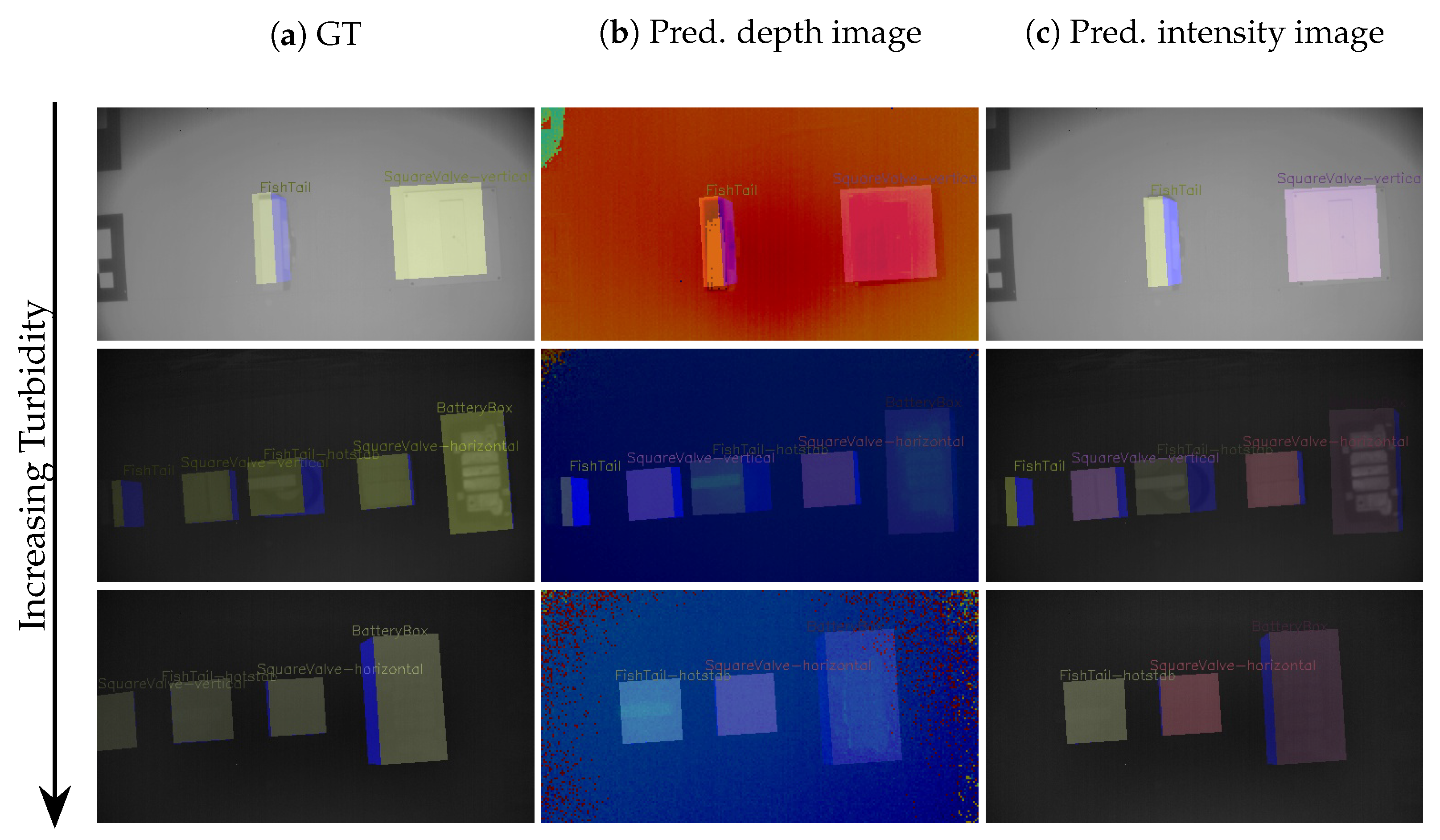To the best of our knowledge, our approach is the first holistic method achieving competitive performance on varying turbidity with multiple objects for sub-sea application [13,14,15]. To visualize the estimated pose on the test dataset, we project the eight corners of the 3D bounding box of the predicted object with the estimated rotation and translation vector and visualize them in Figure 5. The last row shows some of failure cases where it fails to detect objects with limited view and turbidity.

4.1. Evaluation on Intensity, Depth and Fusion Data

We investigate pose estimation performance under different turbidities to shed more light on the proposed model, to objectively evaluate the contribution of intensity, depth and fusion networks against the test datasets, and evaluate the performance in terms of the mAP, RTE and RRE. To this end, we devised prediction performance comparison models, namely, Intensity-Only, Depth-Only, and Fusion. In the Intensity-Only model, the pose estimation network is a single stream network with only intensity image as an input. The intensity image is single channel (gray scale) with a size of $(480\times 256)$. The designed EfficientNet encoder takes an input of size $(512\times 512)$; therefore, the intensity image is padded with zeros to a fixed size of $(512\times 512)$. In the Depth-Only model, the input to the network is only depth image. Similar to the intensity, the depth image is a single channel of $(480\times 256)$ depth values normalized to [0,1]. The depth image is padded with zeros to a fixed size of $(512\times 512)$ similar to intensity image. In the fusion model, both intensity and depth data are fused as discussed in Section 3 and shown in Figure 4. Both intensity and depth images are passed through two EfficientNet encoders. The features from both encoders are fused at different resolution and passed to BiFPN. For all our experiments hyperparameters such as learning rate, batch size, data augmentation remain the same as described in Section 3.4.

Table 2. Two-dimensional Object detection performance (AP) using intensity, depth, fusion.

Turbidity	Method	AP	Fish-Tail	Square-Valve-Vertical	Fish-Tail-Hotstab	Square-Valve-Horizontal	Battery-Box
Turbidity1	Intensity Only	0.90	0.90	0.89	0.89	0.92	0.92
	Depth Only	0.91	0.92	0.90	0.88	0.92	0.90
	Fusion	0.91	0.89	0.91	0.89	0.93	0.94
Turbidity3	Intensity Only	0.90	0.92	0.91	0.89	0.87	0.93
	Depth Only	0.91	0.94	0.90	0.89	0.88	0.93
	Fusion	0.91	0.92	0.90	0.89	0.88	0.97
Turbidity6	Intensity Only	0.90	0.92	0.86	0.89	0.86	0.96
	Depth Only	0.89	0.91	0.87	0.84	0.86	0.94
	Fusion	0.91	0.90	0.91	0.87	0.87	0.97
Overall	Intensity Only	0.90	0.91	0.89	0.89	0.88	0.94
	Depth Only	0.90	0.92	0.89	0.87	0.89	0.92
	Fusion	0.91	0.90	0.91	0.88	0.89	0.96

,

Table 3. Per class translation error (RTE) in $cm$ for the test dataset. The results are averaged over all acquisition.

Turbidity	Method	Avg	Fish-Tail	Square-Valve-Vertical	Fish-Tail-Hotstab	Square-Valve-Horizontal	Battery-Box
Turbidity1	Intensity Only	6.55	6.32	7.01	7.13	6.12	6.16
	Depth Only	6.07	5.40	6.65	6.23	6.25	5.81
	Fusion	6.54	8.78	5.87	5.41	5.72	6.92
Turbidity3	Intensity Only	6.72	6.87	6.88	6.95	6.27	6.62
	Depth Only	6.05	5.19	6.45	6.18	6.59	5.83
	Fusion	6.61	8.58	5.52	5.40	6.07	7.49
Turbidity6	Intensity Only	6.98	7.29	6.89	7.24	6.59	6.91
	Depth Only	6.28	5.37	6.61	6.67	7.00	5.73
	Fusion	6.33	7.89	5.48	5.37	5.92	6.97
Overall	Intensity Only	6.75	6.83	6.93	7.11	6.33	6.56
	Depth Only	6.13	5.32	6.57	6.36	6.61	5.79
	Fusion	6.49	8.42	5.62	5.39	5.90	7.13

and

Table 4. Per class rotation error(RRE) in degree (${}^{\circ }$) for the test dataset. The results are averaged over all acquisition.

Turbidity	Method	Avg	Fish-Tail	Square-Valve-Vertical	Fish-Tail-Hotstab	Square-Valve-Horizontal	Battery-Box
Turbidity1	Intensity Only	3.06	2.64	3.32	2.61	3.83	2.90
	Depth Only	2.93	2.64	3.10	2.45	3.43	3.02
	Fusion	2.62	2.19	3.05	2.42	2.72	2.68
Turbidity3	Intensity Only	3.01	2.75	3.18	2.60	3.73	2.80
	Depth Only	2.87	2.66	2.99	2.46	3.31	2.94
	Fusion	2.56	2.26	2.85	2.44	2.69	2.58
Turbidity6	Intensity Only	2.98	2.75	3.18	2.60	3.63	2.73
	Depth Only	2.91	2.67	3.03	2.57	3.40	2.86
	Fusion	2.59	2.29	2.87	2.46	2.80	2.52
Overall	Intensity Only	3.02	2.71	3.23	2.60	3.73	2.81
	Depth Only	2.90	2.66	3.04	2.49	3.38	2.94
	Fusion	2.59	2.25	2.92	2.44	2.74	2.59

summarize the 2D object detection and pose estimation performances for intensity only, depth only and fusion networks. The results demonstrate that the object detection and rotation estimation performance improved when fusing the intensity and depth image subnetworks. Furthermore, it can be concluded that the rotation error can be reduced optimally by ${0.427}^{\circ }$ on average over all turbidities by combining the intensity and the depth subnetworks. However, the translation error is reduced by 0.36 cm as compared to using only depth. In summary, the 2D and rotation predictions obtained by fusing depth and intensity subnetworks are found to be complementary, and the fusion model can obtain more accurate 6D pose estimation.

4.2. Dataset Bias Analysis

We further analyse the capture bias problem [26] (generalization beyond the training domain) in order to explore the limitation and performance of the proposed approach as well as the dataset. The capture bias is related to how the images are acquired both in terms of turbidity and of the collector preferences for point of view, lighting, etc. Table 1 shows the proposed approach is able to generalize to novel turbidity that is not in the training dataset. Compared to related works [13,14,15], the proposed model is robust to different turbidity levels. In regard to preference for view point, Figure 6 shows the variation of rotation error with respect to ground truth euler angles of each object along X, Y and Z axis.

The ground truth mean rotation angle of the test dataset distribution is shown in the right side Y axis of Figure 6. We observe that the rotation error varies with a span of dataset capturing setup more in high turbidity. This is expected in that, in high turbid cases 6D pose estimation requires large amount of data for a better generalization. Overall, the proposed model is able to generalize in high turbidity cases with mAP score above 90% as show in Table 1.

4.3. Discussion

The ability to detect and localize objects underwater is a crucial step for subsea inspection, maintenance and repair operations. The results presented earlier in this section revealed that the pose estimation errors exhibit variation in performance with object size, data capture bias and turbidity. Large objects such as battery box are easy to detect as compared to small objects ($+\Delta 5\%$) AP. Increasing capturing device image resolution as well as models input resolution could help boost the performance. Using 3D vision reduces the rotation and translation error by ${0.39}^{\circ }$ and $6.5$ mm, respectively, as compared to 2D vision. However, the rotation sub-network is benefited more from 3D vision than translation sub-network. This is due to the fact that there is a small deviation between object location in the intensity and depth images during fast movement of the capturing setup. Performance drop on high turbidity water could be mitigated by including high turbidity examples for training the network (i.e., we used turbidity 0, 2, 4, 5, and 7 for training and turbidity 1, 3 and 6 for testing). Lastly, dataset capture bias related to view point selection in 3D pose estimation could also impact the performance of the proposed method. Figure 6 shows that the rotation values are not evenly represented in the datasets. This is seen in conjunction with turbidity values and prediction error in the rotation. It appears that, the largest errors of the pose estimates occur in the high turbidity and with less represented pose values in the training dataset. In practical settings, such issues need to be addressed if one is to build a system that works outside of well calibrated laboratory setups and datasets. Data capture bias can emanate from automated data labelling process. Recall from Section 2.1 that the process of labelling the datasets was automated and based on real-sense camera detected Aruco markers mapped by a time-stamp to the locations in the images of the Utofia camera. The transformation between the two cameras could result in small drift depending on the speed of capturing setup, which in turn results in miss-aligned bounding boxes. It is uncertain how these incorrect pose labels affect the performance of the network. It is also possible that there will be outliers in the training/test dataset with small bounding box and pose deviation. Moreover, such deviation in the test set could affect the results as the network will not predict the corresponding incorrect values. However, for the training and test data, we have filtered frames with large displacement and trained only clean version of the dataset (using only frames were the capturing setup is relatively stationary). We have checked visually that such deviations occur in a few samples out of thousands in the training sets, and should therefore not have a too big impact.

5. Conclusions

In this work, we introduce an efficient automated data annotation approach to train deep learning models for underwater pose estimation. Furthermore, we proposed an end-to-end deep learning model that is able to estimate 6D pose using 3D vision under different turbidity levels. The method couples object detection with 6D pose (translation and rotation) estimation using shared encoder, making it more efficient than previous two-stage approaches. The results showed that the proposed model is able to detect and estimate underwater objects 6D pose with 91% mAP and 2.59${}^{\circ }$ and 6.5 cm deviation in rotation and translation, respectively. The proposed approach runs at 16 frames per second on a single GPU (GeForce RTX 2080 Ti, 11 GB) and is able to handle multiple objects without computational time increase.

References

1. Hodan, T.; Michel, F.; Brachmann, E.; Kehl, W.; GlentBuch, A.; Kraft, D.; Drost, B.; Vidal, J.; Ihrke, S.; Zabulis, X.; et al. Bop: Benchmark for 6d object pose estimation. In Proceedings of the European Conference on Computer Vision (ECCV), Munich, Germany, 8–14 September 2018; pp. 19–34. [Google Scholar]
2. Castillón, M.; Palomer, A.; Forest, J.; Ridao, P. State of the art of underwater active optical 3D scanners. Sensors 2019, 19, 5161. [Google Scholar] [CrossRef] [PubMed] [Green Version]
3. Risholm, P.; Thorstensen, J.; Thielemann, J.T.; Kaspersen, K.; Tschudi, J.; Yates, C.; Softley, C.; Abrosimov, I.; Alexander, J.; Haugholt, K.H. Real-time super-resolved 3D in turbid water using a fast range-gated CMOS camera. Appl. Opt. 2018, 57, 3927–3937. [Google Scholar] [CrossRef] [PubMed]
4. He, Z.; Feng, W.; Zhao, X.; Lv, Y. 6D Pose Estimation of Objects: Recent Technologies and Challenges. Appl. Sci. 2021, 11, 228. [Google Scholar] [CrossRef]
5. Xiang, Y.; Schmidt, T.; Narayanan, V.; Fox, D. Posecnn: A convolutional neural network for 6d object pose estimation in cluttered scenes. arXiv 2017, arXiv:1711.00199. [Google Scholar]
6. Labbé, Y.; Carpentier, J.; Aubry, M.; Sivic, J. CosyPose: Consistent multi-view multi-object 6D pose estimation. In European Conference on Computer Vision; Springer: Berlin/Heidelberg, Germany, 2020; pp. 574–591. [Google Scholar]
7. Bukschat, Y.; Vetter, M. EfficientPose—An efficient, accurate and scalable end-to-end 6D multi object pose estimation approach. arXiv 2020, arXiv:2011.04307. [Google Scholar]
8. Tan, M.; Pang, R.; Le, Q.V. Efficientdet: Scalable and efficient object detection. In Proceedings of the IEEE/CVF Conference on Computer Vision and Pattern Recognition, Seattle, WA, USA, 13–19 June 2020; pp. 10781–10790. [Google Scholar]
9. Wang, C.; Xu, D.; Zhu, Y.; Martín-Martín, R.; Lu, C.; Fei-Fei, L.; Savarese, S. DenseFusion: 6D Object Pose Estimation by Iterative Dense Fusion. In Proceedings of the Computer Vision and Pattern Recognition (CVPR), Long Beach, CA, USA, 16–20 June 2019. [Google Scholar]
10. He, Y.; Sun, W.; Huang, H.; Liu, J.; Fan, H.; Sun, J. Pvn3d: A deep point-wise 3d keypoints voting network for 6dof pose estimation. In Proceedings of the IEEE/CVF Conference on Computer Vision and Pattern Recognition, Seattle, WA, USA, 13–19 June 2020; pp. 11632–11641. [Google Scholar]
11. Jeon, M.; Lee, Y.; Shin, Y.S.; Jang, H.; Kim, A. Underwater object detection and pose estimation using deep learning. IFAC-PapersOnLine 2019, 52, 78–81. [Google Scholar] [CrossRef]
12. He, K.; Gkioxari, G.; Dollár, P.; Girshick, R. Mask r-cnn. In Proceedings of the IEEE International Conference on Computer Vision, Venice, Italy, 22–29 October 2017; pp. 2961–2969. [Google Scholar]
13. Martin-Abadal, M.; Piñar-Molina, M.; Martorell-Torres, A.; Oliver-Codina, G.; Gonzalez-Cid, Y. Underwater Pipe and Valve 3D Recognition Using Deep Learning Segmentation. J. Mar. Sci. Eng. 2021, 9, 5. [Google Scholar] [CrossRef]
14. Qi, C.R.; Su, H.; Mo, K.; Guibas, L.J. Pointnet: Deep learning on point sets for 3d classification and segmentation. In Proceedings of the IEEE Conference on Computer Vision and Pattern Recognition, Honolulu, HI, USA, 21–26 July 2017; pp. 652–660. [Google Scholar]
15. Nielsen, M.C.; Leonhardsen, M.H.; Schjølberg, I. Evaluation of posenet for 6-dof underwater pose estimation. In Proceedings of the OCEANS 2019 MTS/IEEE SEATTLE, Seattle, WA, USA, 27–31 October 2019; IEEE: Piscataway, NJ, USA, 2019; pp. 1–6. [Google Scholar]
16. Kendall, A.; Grimes, M.; Cipolla, R. Posenet: A convolutional network for real-time 6-dof camera relocalization. In Proceedings of the IEEE International Conference on Computer Vision, Santiago, Chile, 7–13 December 2015; pp. 2938–2946. [Google Scholar]
17. OpenCV. OpenCV: Detection of ArUco Markers. Available online: https://docs.opencv.org/3.4/d5/dae/tutorial_aruco_detection.html (accessed on 14 June 2021).
18. Szeliski, R. Computer Vision: Algorithms and Applications; Springer Science & Business Media: Berlin/Heidelberg, Germany, 2010. [Google Scholar]
19. Kang, L.; Wu, L.; Yang, Y.H. Experimental study of the influence of refraction on underwater three-dimensional reconstruction using the svp camera model. Appl. Opt. 2012, 51, 7591–7603. [Google Scholar] [CrossRef] [PubMed]
20. Tan, M.; Le, Q. Efficientnet: Rethinking model scaling for convolutional neural networks. In Proceedings of the International Conference on Machine Learning, Long Beach, CA, USA, 10–15 June 2019; PMLR: Cambridge, MA, USA, 2019; pp. 6105–6114. [Google Scholar]
21. Zhou, Y.; Barnes, C.; Lu, J.; Yang, J.; Li, H. On the continuity of rotation representations in neural networks. In Proceedings of the IEEE/CVF Conference on Computer Vision and Pattern Recognition, Long Beach, CA, USA, 15–20 June 2019; pp. 5745–5753. [Google Scholar]
22. Elfwing, S.; Uchibe, E.; Doya, K. Sigmoid-weighted linear units for neural network function approximation in reinforcement learning. Neural Netw. 2018, 107, 3–11. [Google Scholar] [CrossRef] [PubMed]
23. Liu, W.; Anguelov, D.; Erhan, D.; Szegedy, C.; Reed, S.; Fu, C.Y.; Berg, A.C. Ssd: Single shot multibox detector. In European Conference on Computer Vision; Springer: Berlin/Heidelberg, Germany, 2016; pp. 21–37. [Google Scholar]
24. Elbaz, G.; Avraham, T.; Fischer, A. 3D point cloud registration for localization using a deep neural network auto-encoder. In Proceedings of the IEEE Conference on Computer Vision and Pattern Recognition, Honolulu, HI, USA, 21–26 July 2017; pp. 4631–4640. [Google Scholar]
25. Everingham, M.; Van Gool, L.; Williams, C.K.; Winn, J.; Zisserman, A. The pascal visual object classes (voc) challenge. Int. J. Comput. Vis. 2010, 88, 303–338. [Google Scholar] [CrossRef] [Green Version]
26. Yamada, M.; Sigal, L.; Raptis, M. No bias left behind: Covariate shift adaptation for discriminative 3d pose estimation. In European Conference on Computer Vision; Springer: Berlin/Heidelberg, Germany, 2012; pp. 674–687. [Google Scholar]
Figure 1. Experimental setup and objects of interest. (a) shows capturing setup. Realsense and Utofia cameras are time synced, and the projection between the two cameras is established using known locations of the Aruco markers. (bf) shows typical objects such as valves, fish-tails, stab-connector, and gauges that are common in sub-sea inspection.
Electronics 10 02369 g001
Figure 2. Subsea panel with projected ground truth pose as seen across turbidities. Images were acquired under seven different turbidites, ranging from 8.3 m down to 2.2 m attenuation length.
Electronics 10 02369 g002
Figure 3. Range-gated 3D camera system. The full system includes a top-side box, Gigabit Ethernet cable, PC, and a cylindrical underwater housing.
Electronics 10 02369 g003
Figure 4. Overview of the proposed 6D pose estimation network. Input features are extracted from intensity and depth image with an EfficientNet [20] encoder. Features from both streams are fused at different scales and passed to bidirectional feature pyramid networks (BiFPN) and the prediction subnetworks. Both intensity and depth input images are the size of ( 512 × 512 ) . The output shape for bbox regression, classification, 6D regression and translation heads are 4 × N c , 1 × N c , 6 × N c and 3 × N c , respectively, where N c is the number of anchor boxes used for object detection.
Electronics 10 02369 g004
Figure 5. Qualitative results for detection and pose estimation: The first column (a) shows ground truth pose projected on the intensity images. Column two (b) and three (c) shows the estimated pose projected on the depth and intensity image, respectively. The top, middle and last row shows ground truth and predicted pose result for turbidities 1, 3 and 6. The last row shows miss-detection (i.e., four object in GT and three detected objects in the prediction) under partial occlusion and low depth resolution. The processing time for a single frame is 62.5 ms or 16 frames per second using a single GPU (GeForce RTX 2080 Ti, 11 GB).
Electronics 10 02369 g005
Figure 6. Fusion model pose estimation (rotation and translation) error with respect ground truth data distribution for various turbidities. The top, middle and last row shows ground truth rotation angles vs. error in rotation for turbidities 1, 3 and 6, respectively.
Electronics 10 02369 g006