Applying a Genetic Algorithm to a m-TSP: Case Study of a Decision Support System for Optimizing a Beverage Logistics Vehicles Routing Problem

Abstract

Route optimization has become an increasing problem in the transportation and logistics sector within the development of smart cities. This article aims to demonstrate the implementation of a genetic algorithm adapted to a Vehicle Route Problem (VRP) in a company based in the city of Covilhã (Portugal). Basing the entire approach to this problem on the characteristic assumptions of the Multiple Traveling Salesman Problem (m-TSP) approach, an optimization of the daily routes for the workers assigned to distribution, divided into three zones: North, South and Central, was performed. A critical approach to the returned routes based on the adaptation to the geography of the Zones was performed. From a comparison with the data provided by the company, it is predicted by the application of a genetic algorithm to the m-TSP, that there will be a reduction of 618 km per week of the total distance traveled. This result has a huge impact in several forms: clients are visited in time, promoting provider-client relations; reduction of the fixed costs with fuel; promotion of environmental sustainability by the reduction of logistic routes. All these improvements and optimizations can be thought of as contributions to foster smart cities.

1. Introduction

The concern for the development of smart cities has been growing exponentially in recent years. The smart city concept may vary, but it is mostly focused on the environment, and its preservation, and not only on the technology, as described by Aletà et al. [1]. It can also be based on three main concepts: economic efficiency, social equity, and, the most relevant, environmental quality [2]. The increasing need to make cities more sustainable and designed for people has led to the search for alternatives that allow for a better rationalization and optimization of resources and means. These developments in cities have not only had an effect on their design and organization but also play a very important role in promoting development, for example, in industry and in the way communities perceive their activities. Smart Mobility, as some authors refer to it, may be perceived through the optics of the transportation of people or goods. The growth of the cities and the importance of mobility within the urban area has led to research on ways to minimize traffic, its impact on the environment, and increase the efficiency of travel. The industry’s evolution has also increased the concern to improve the profitability of resources, in order to reduce costs and increase efficiency, keeping up with the main concerns of the evolution of smart cities. Despite being a constantly changing problem, due to instabilities of a different kind, business success can often be dictated by the applied methodology. With the growing need for the enhancement of the efficiency associated with the transportation of goods, logistics has become a very important economic activity.

Logistics can be defined as the art and science of acquiring, producing, and distributing all products considering the usefulness of time and place, that is, the timing of delivery at the right place and not only in the shortest time possible but also at the right time [3]. Companies specialized in logistical processes can focus on different areas, such as transporting goods and some additional services, such as warehouse management or stock control. Although transportation is the main focus of this sector, it is also very important to control the stock and manage the storage of products. Thus, decision support systems play a very important role in this management.

It is possible to observe an increasing interconnection between linear programming and problems in goods transportation, most of the time related to the question: What would be the best shipping method that allows a minimized cost of shipping of n units to m destinations and a maximization of the profit? Several methods are available. Vehicle Route Problem (VRP) is based on the assignment of distribution routes for a set of clients scattered on the map at the lowest possible cost [4]. The Traveling Salesman Problem (TSP) seeks to define routes that cover all points of sale, passing through each one only once, returning to the point of origin. The Multiple Traveling Salesman Problem (m-TSP) is a variant of the TSP. The difference is the existence of m sellers for n destinations. Since the beginning of the TSP study, many approaches and methods have been developed [5]: classic methods, mainly based on linear programming [6] and branch-and-bound [7], and artificial intelligence methods, such as Tabu Search, Genetic Algorithms or Artificial Neural Networks. Artificial intelligence methods based on neural networks represent a good approach to the problem in this study, as they are not less effective than others. Their characteristics allow the needed calculations to occur, even when conditions change over time [8]. If a complex problem of the shortest path is not approached using a neural network or genetic algorithms, the complexity of the problem grows exponentially.

Sakharov et al. [9] consider that a large number of empirical problems can be formulated as problems of finding the shortest path and can be solved using network models, once again, recurring to artificial intelligence methods. A universal computer model of the Floyd–Warshall algorithm was used to approach a shortest path problem. All steps that the algorithm takes to return a solution were described, providing a tree of points. However, the Floyd–Warshall algorithm is not the best approach to this problem, specifically because of the characteristics of the user data. This type of algorithm works better in cases of weighted, oriented or not, graphs, opposed to this problem in which the simplification of the roads and establishments to nodes and edges could return a non-applicable solution.

Azis et al. [10] conducted a study whose main objective was to compare the conventional methods, the Floyd–Warshall Algorithm and the Heuristic Method, the so-called Greedy Algorithm. Through the data analysis and interpretation, it was possible to conclude that the conventional method, despite its “temporal” limitations in defining the shortest route, compared to the greedy algorithm, is more accurate. Although taking longer, it considers all stopping points and possible routes, while the greedy algorithm exclusively recognizes the one with the lowest weight in each interaction, so that the time frame is smaller and consequently always leading to the optimal final result. Hybrid methods can also be applied. Jiang et al. [11] proposed a hybrid method, merging the Ant Colony Algorithms (ACO) and the Partheno Genetic Algorithms (PGA), similar to the Genetic Algorithms, but lacking the crossover operators. The ACO are known for being suitable for NP-hard problems, such as m-TSP, and the PGA are a great approach to this kind of problem [12]. The complexity level of the current case study does not require such a method.

Fujdiak et al. [13] applied genetic algorithms in a real case study of waste collecting in smart cities context as an optimization method. A crossover and mutation of the Floyd–Warshall algorithm was performed. This algorithm was chosen since a metric system was used and the negative values of edges are not used. The crossover allowed to develop changes in the new population and consequently find a better solution. The mutations allowed to exchange nodes. As in our case study, asymmetric matrices considering the existence of one-way streets were resorted to. Despite being similar case studies, this algorithm does not apply to the current problem since despite generating the solution for the shortest distance between all pairs of vertices, it was applied to a problem with a smaller sample size.

The m-TSP problem is an approach that softens the VRP problem when it comes to capacity but is nevertheless able to address other needs, such as single or multiple warehouse constraints, numbers of vendors, work schedule constraints or limits on locations per vendor, and even time window constraints. These types of problems are not only useful for managing vendor routes, but also for other purposes where more informed decision-making is useful. Solving this problem can be used, for example, to distribute work among several workers with restricted functions, by managing their schedules, by planning missions or production, or by distributing tasks efficiently [14]. We seem to be moving towards times when, for example, unmanned aerial vehicles, known as drones, will play a fundamental role in short distribution routes for light load or for transportation within industrial complexes. The m-TSP problem using aerial vehicles is addressed in [15]. New approaches will be required to deal effectively with these kind of problems.

It is also usual to observe that some of these routing problems are dynamic, in which the cities or places to visit are known over time and not in advance as in conventional vehicle routing problems. Gam [16] addressed two different heuristics, proposing in one the assignment of the vehicle with the shortest distance traveled to the client, and in the other, the vehicle that is closest to the new location that arose in the problem. These heuristics also pay attention to the number of locations to visit so that all salesmen visit roughly the same number.

There are numerous applications for dynamic m-TSP problems, such as pickup and delivery services where several time windows and vehicle waiting times are present [17]. This is already an evolution from one of the pioneering studies [18] in which it was not taken into account that deliveries can all influence each other directly by changing all delivery times.

Based on methods already developed, such as VRP, TSP, m-TSP, combined with Genetic Algorithms (GA), it was possible to obtain the best route to follow in order to minimize costs [19]. A GA is a meta-heuristic method that does not work with single optimal solutions, but with populations of solutions [20].

2. Methodology

The m-TSP is a well-known extension of the traveling salesman problem, in which n cities are assigned to m sellers, where each knot can only be visited once by only one seller, thus preventing route overlapping. It is necessary to pay attention to the limitations to which the problem is subject, such as, for example, damaged roads or tolls, timetables and temporal windows, precedence in deliveries, etc. In this case study, the biggest constraint is the minimum number of places to be visited [15].

The mathematical model of m-TSP can be represented through the following formulation:

$$Minimization:F=\left(f_1,f_2\right)$$

(1)

$$f_1={\sum }_{k=1}^m{\sum }_{i=0}^n{\sum }_{j=1}^n{c}_{ij}{x}_{ijk}$$

(2)

$$f_2=\underset{0\le x\le 1}{\mathit{max}}{\sum }_{i=0}^n{\sum }_{j=0}^n{c}_{ij}{x}_{ijk}-\underset{1\le k\le m}{\mathit{min}}{\sum }_{i=0}^n{\sum }_{j=0}^n{c}_{ij}{x}_{ijk}$$

(3)

where,

$$x_{ij}=\{\begin{array}{c}1, salesmene K goes from city i to city j \\ 0, otherwise\end{array}$$

(4)

$$s.t.\{\begin{array}{l}{\sum }_{k=1}^m{\sum }_{i=0}^n{x}_{ijk}=1; \forall j=1\dots \dots ,\mathrm{n}\\ {\sum }_{k=1}^m{\sum }_{j=0}^n{x}_{ijk}=1; \forall j=1\dots \dots ,\mathrm{n}\\ \hspace{1em}\hspace{1em}\hspace{1em}{\sum }_{k=1}^m{\sum }_{i=1}^n x_{i0k}=m\\ \hspace{1em}\hspace{1em}\hspace{1em}{\sum }_{k=1}^m{\sum }_{j=1}^n x_{i0k}=m\\ {\sum }_{i\in S}{\sum }_{j\notin S}{x}_{ijk}\ge 1; \forall k\in V,\forall S\subseteq C\end{array}$$

(5)

The information above is represented by the set of n cities and m sellers and is expressed by

$$C=\left(i\right), i=0, 1, 2, \dots , n; V=\left(k\right), k=1, 2, \dots , m.$$

(6)

where c_ij defines the distance between cities i and j, and x_ijk for the salesman k from cities i to j, considering that each city is visited only once [21].

Equations (2) and (3) represent, respectively, the two objective functions that are intended to be minimized: the total distance from the seller and the difference between the longest and shortest route. Equation (5) concerns the restriction that all salesmen depart from the same city. So, except at the point of origin, there is only one salesman at each point.

Through a previous analysis of the various types of algorithms and methods available, it is concluded that, for problems of this type, the best approach is to use Genetic Algorithms. Genetic Algorithms are meta-heuristic methods that are based on scientific phenomena, such as the Theory of the Evolution of Species, in which each one has a variety of individuals, with some characteristics being maintained in generations and others recombined. This type of algorithm does not work with single optimal solutions, but with a population of solutions, which are improved over time, as only individuals with the best characteristics survive and predominate [20]. 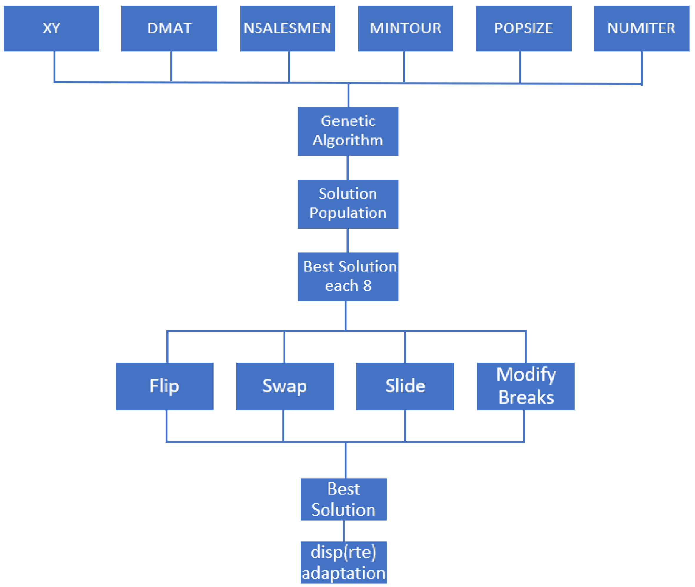The Genetic Algorithm developed by Kirk [22] finds a viable solution close to the optimal solution for m-TSP, one of the TSP variations, which looks for the shortest route passing through all points of a network. This algorithm is based on two important premises: (a) it is a closed m-TSP, that is, the starting point is also the return point, in this case, the company’s headquarters; (b) Except for the starting point, each location is only visited once. Before the iterative process, it is necessary to define the characteristic inputs of this algorithm:

• Generate XY, an N × 2 matrix, where N is the number of places, in which it was chosen to generate a “random” matrix of N × N. Thus, the results of the solution will be later portrayed on a map, instead of having to insert a matrix with the coordinates of each place.
• Insert DMAT, which is the N × N matrix of distances or costs. Distances between locations were looked up on Google Maps and imported in Microsoft Excel matrices.
• NSALESMEN represents the number of vendors visiting the locations, which differ in this problem between one salesman on the large experimental routes, two salesmen on the routes in the North and South zones and four in the Central area.
• MINTOUR is the minimum number of places to be visited by each salesman, in this case 10 locations on all routes except Central Route which was defined as 15 as there are more places. It was through this input that the number of places to visit per day, for each salesman, was kept balanced.
• POPSIZE was set to 80, which represents the number of solutions with which the algorithm starts iterations and mutations in search of a better solution. This parameter must be, by obligation of the algorithm, divisible by 8.
• NUMITER is the maximum number of iterations that the algorithm will do, in search of the best solution, in which case it was defined as 5000.
• The remaining inputs, were kept unchanged, remaining by default.

It was also necessary to make an adjustment to the code of the algorithm, in which a “disp(rte)” was inserted, a function that allows the viewing of the order of the points of the returned routes. Contrary to the original code, where only the visual format of the connections and the total sum of kilometers of the solution’s routes existed, this not being viable because a random matrix was used instead of a matrix of geographic coordinates.

The algorithm flowchart shown in Figure 1 helps to understand how the algorithm works, in which the necessary inputs are initially inserted. After defining the inputs, the algorithm will choose the best solution from the initial population of eight. With this more restricted group of solutions, it will start mutating some parts of the solution through Flip, Swap, Slide and Modify Breaks. With the best solution found and with the adaptation included in the algorithm it is possible to visualize the direction in which to go.

The algorithm was reproduced on an Asus VivoBook computer with Intel(R) Core (TM) i7-8565U CPU @ 1.80 GHz 1.99 GHz, 16.0 GB RAM, Windows 10 Home 64-bit OS. The response time of the various routes was always between 2 s and 10 s. Thus, the computation time is acceptable for real case applications.

3. Case Study

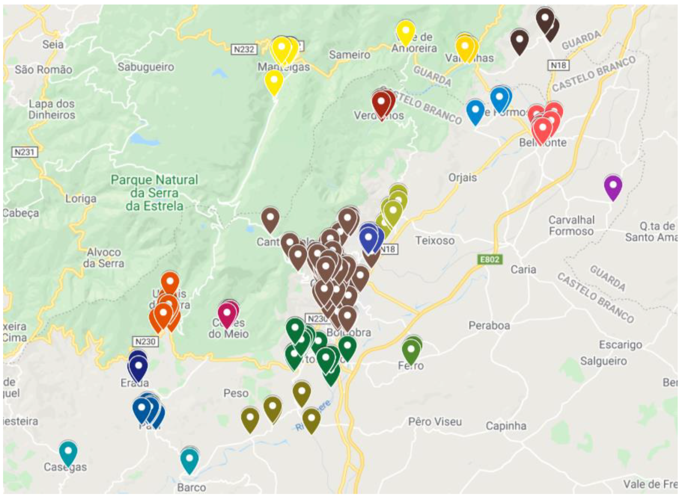
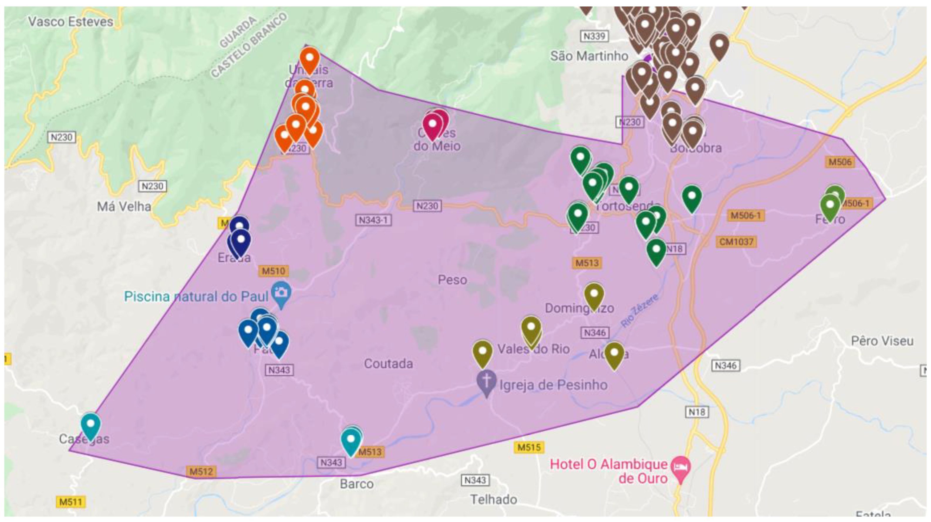
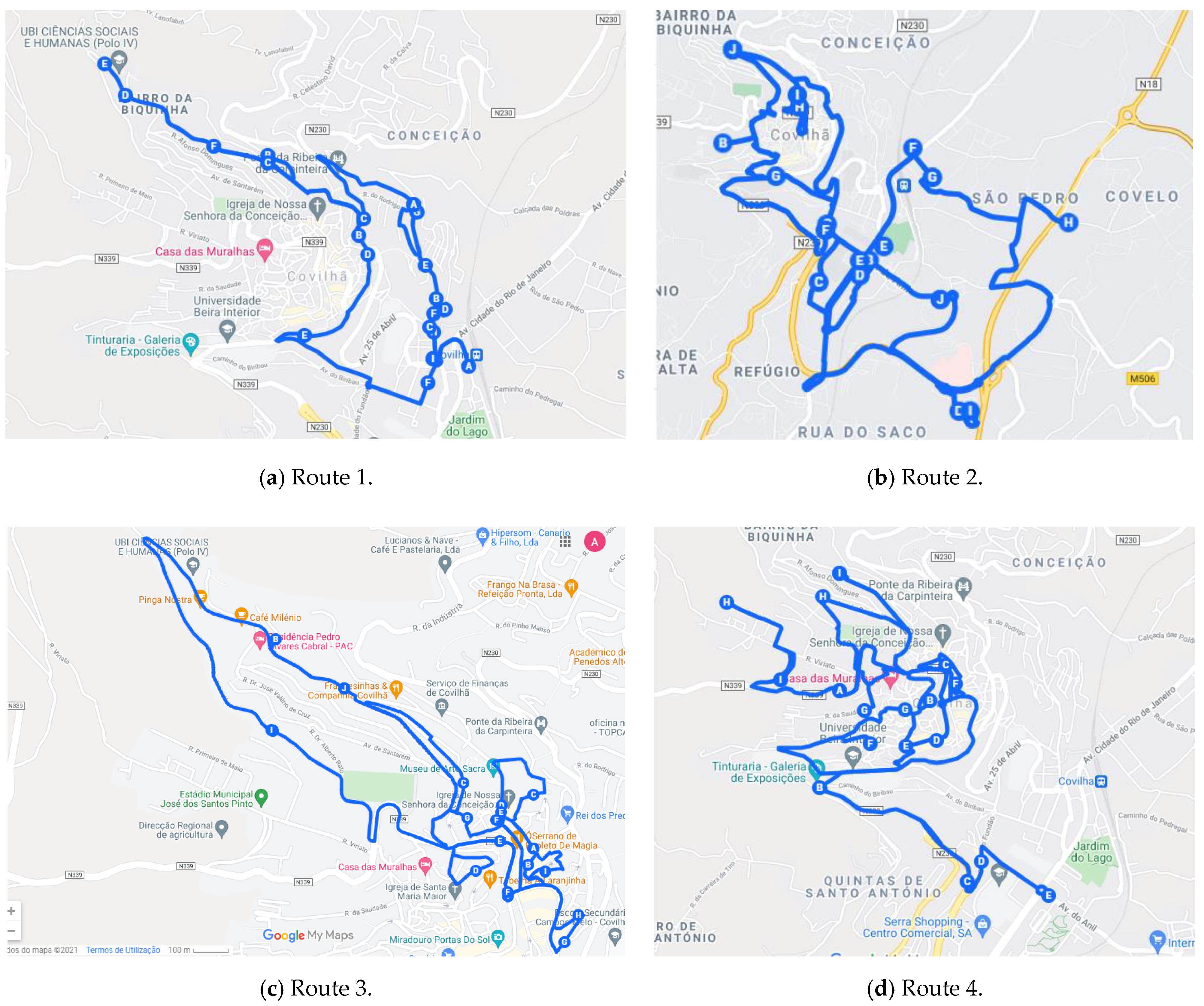
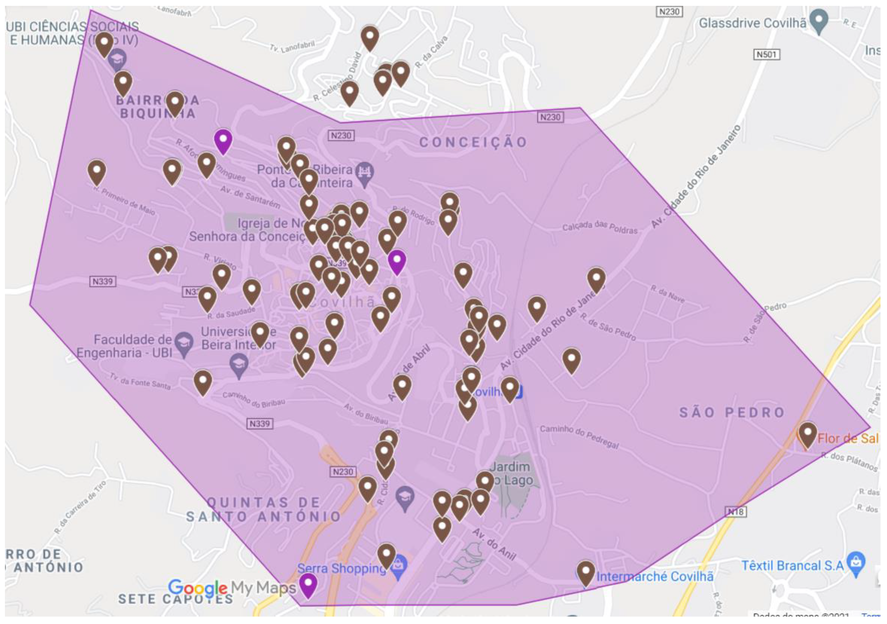
The problem under analysis is the creation of a decision support system (DSS) that allows for the optimization of distribution routes of a small food and beverage distribution company, headquartered in Covilhã, Portugal. The main goal of the DSS is to optimize routes, for the five days of the week, which minimizes travel costs and the distances traveled by workers, considering the approximately 270 establishments provided by the company. These locations can be seen in Figure 2.

Currently, the routes are covered by four workers: one that only carries out sales, another which carries out sales and only distributes the respective orders, one that carries out sales only one day of the week and distributes the rest, and the last that only distributes. However, these task assignments are not reflected on an optimization of the time and distance covered by workers and, therefore, the applied methodology undergoes a reorganization of the distribution of the workers in question. Thus, two workers are allocated to exclusively carry out the sales and the remaining two workers to exclusively carry out the delivery of orders. Following this approach, it was intended to optimize eight routes, one for each seller/distributor, for four days a week, with Friday being destined for locations that, for some reason external to the company, could not be visited.

Currently, there are many factors external to the company that may lead to the need to revisit some of the locations at the end of the week. This way, two routes to the North and South Zones and four routes to the Central Zone will be considered. It is assumed that the distributor can travel the same route that the seller traveled and that, therefore, there will not be a need to create personalized routes. These routes must allow workers to cover the minimum number of total kilometers, but also consider the characteristics of the roads, particularly the orography since the city is located in a mountain region with crooked roads with high slopes. This condition may lead to high fuel consumption and consequently to higher fuel costs besides the significant emission of combustion gases that must be reduced to promote environmental sustainability.

4. Model Formulation

Initially, in order to reduce the complexity of data processing provided by the company, the approximately 270 establishments were divided into three main zones: North Zone, South Zone and Central Zone. A simplification was sought, similarly to the division into three main zones, within the North and South zones because, although there is a wide dispersion of establishments in the zones, it is possible to define some clusters within the locations, since the distances between establishments, compared to the distances between locations, are negligible. Using the Google Maps distance measurement tool, the exact distances between each point were obtained, thus allowing the construction of distance matrices for the respective zones. These matrices of dimension N × N, with N being the number of key points associated with each of the three zones in question, were adapted, resorting, when necessary, to the maximization of distances that would represent conditioned sections, either by the distance they represent or by the conditions of the road necessary to go through. These maximizations were the result of a study of the pattern through the exhaustive iterative running of the algorithm, which was observed in the various routes. Mostly, the algorithm returned a solution that presented a smaller route and a larger one, in the case of the North and South zones. It is considered that these matrices are symmetric, to ease problem-solving. For example, the distance from point A to B is always equal to the distance from point B to A, therefore not considering any types of traffic constraints that may cause significant differences between A to B and vice-versa.

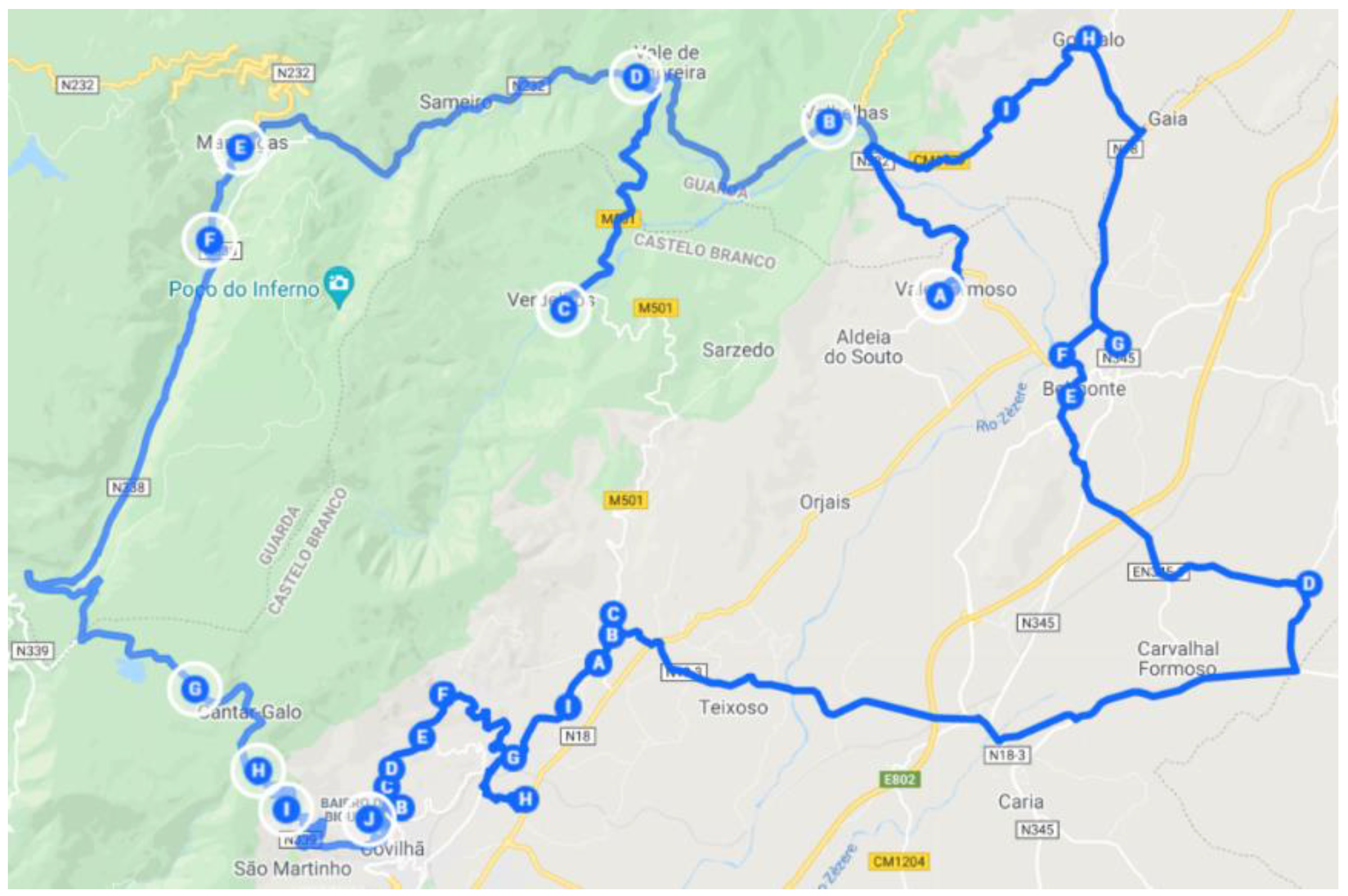
4.1. North Zone

The zone defined as the North Zone has 26 key points. It is possible to observe in Figure 3 and

Table 1. Clusters of North zone.

Clusters (1)	Key Points
Inguias (1)	217
Belmonte (12)	202, 57, 175
Gonçalo (4)	125
Cruz da Pedra (1)	253
Vale Formoso (3)	213
Valhelhas (3)	15
Verdelhos (6)	69
Vale da Amoreira (1)	212
Manteigas (11)	136, 139
Penhas da Saúde (4)	230, 169, 180
Penedos Altos (16)	121, 145, 215, 73
Parque Industrial Canhoso (1)	60
Canhoso (7)	162
Teixoso (10)	148, 229, 261
Gibraltar (1)	103
Vila do Carvalho (5)	52

⁽¹⁾ Number of establishments associated with the cluster.

the many key points associated with the Clusters in question.

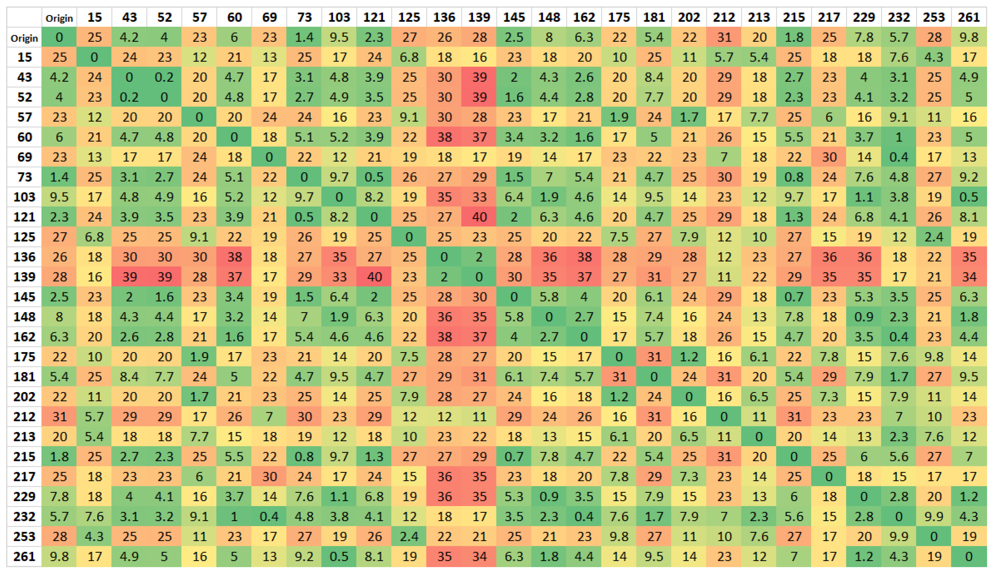
Initially, using the 26 × 26 matrix shown in Figure 4, and considering a single route, with only one salesman, it was evaluated how the algorithm would proceed in the connection between the points. Due to the orography of the area, the first matrix, when used for two salesmen, did not return a viable solution. The solution considered splitting the 26 × 26 distance matrix in two: an outer Route, including the points far away with crooked roads with high slopes, and a smaller Route, encompassing the points closer to the city.

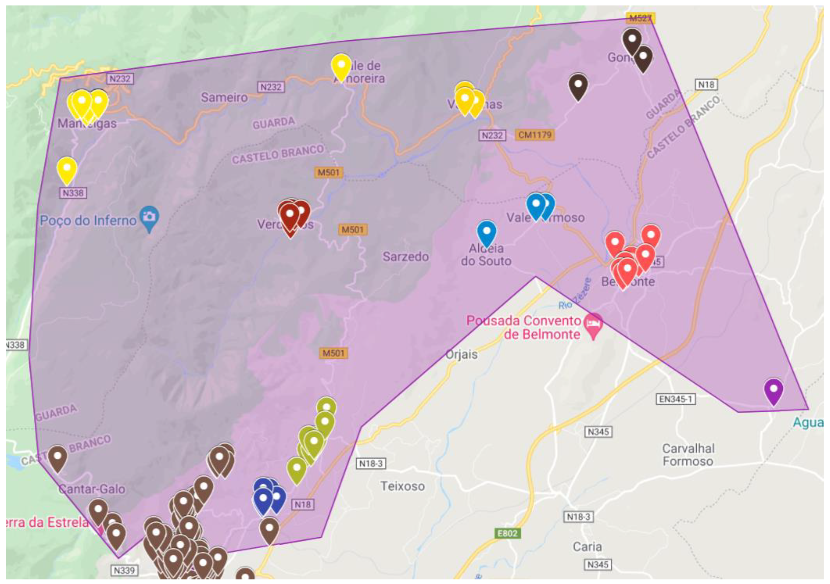
Also, for this main zone, due to the different responses returned by the algorithm, it was necessary to study the possibility of conditioning, through the maximization of values, a specific location of key points and decide to which route it belongs. Thus, through a preliminary analysis, the matrix of this zone was divided into two, with only the points of the routes previously returned, and divided into two approaches: Verdelhos (red dots in Figure 3, corresponding to key point 69) in the inside and the outside route. By applying the algorithm to only one salesman for both approaches, adding the distances of both routes, the solutions were 152.95 km and 139.10 km, for key point 69, inside or outside, respectively. With these data, it was possible to conclude that there was a need to maximize the distances from the cluster associated to point 69 to points further south, thus enforcing it to be inserted in the route of the localities on the outside.

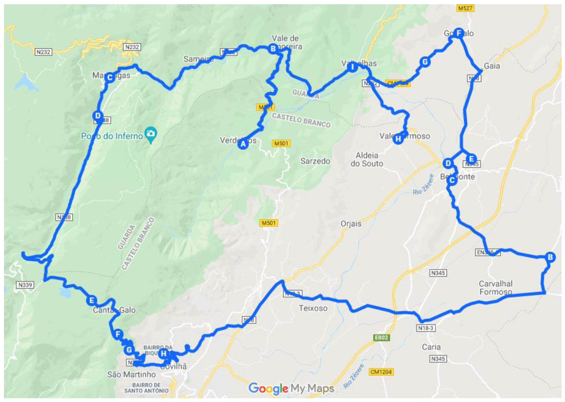
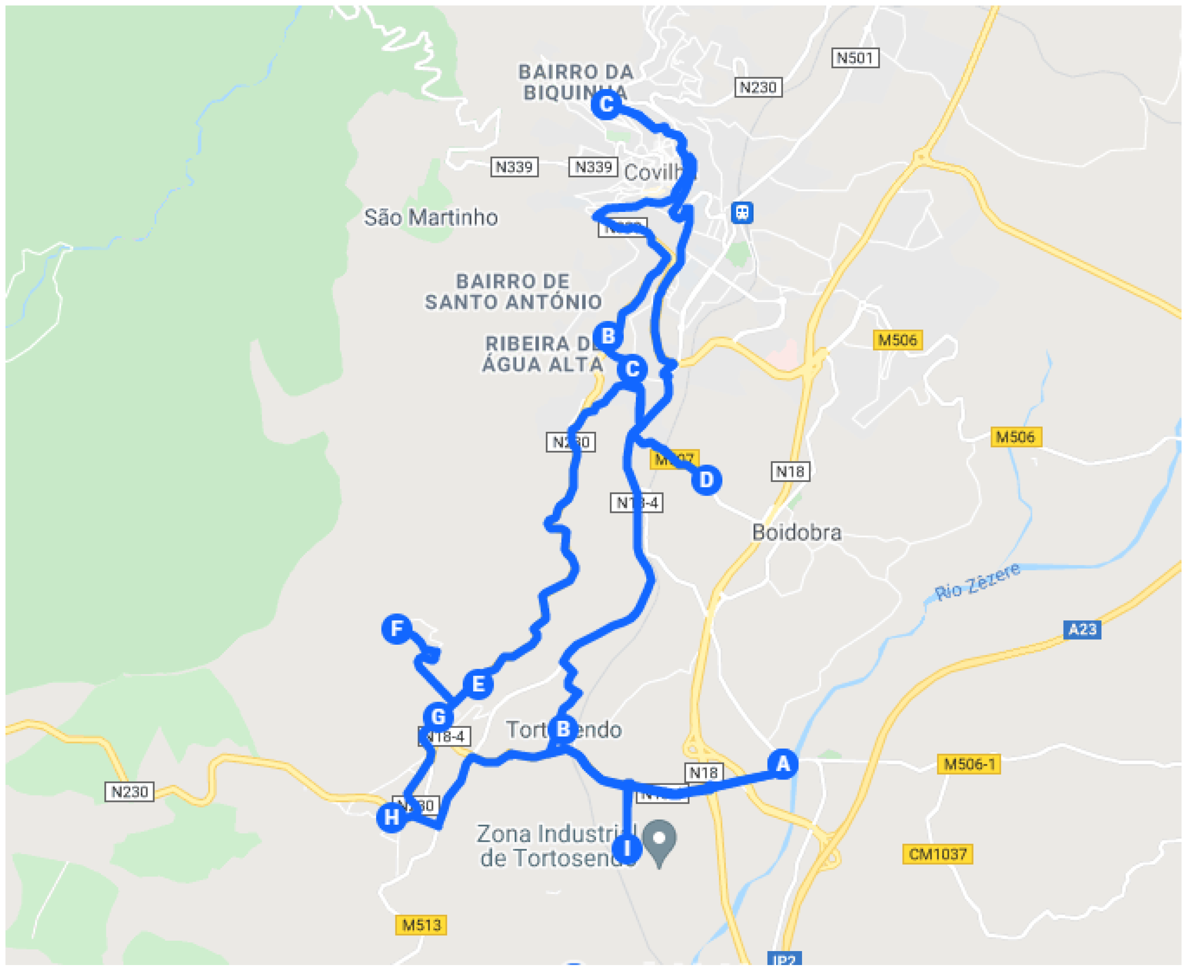
4.2. South Zone

The South Zone also has 26 key points. These can be seen in Figure 5 and

Table 2. Clusters South zone.

Clusters (1)	Key Points
Covilhã Sul (4)	260, 54
Ferro (2)	218
Alcaria (1)	259
Dominguizo (1)	254
Vales do Rio (2)	199
Peso (1)	120
Barco (3)	131
Paul (12)	79, 220
Casegas (1)	44
Erada (3)	101
Unhais da Serra (15)	105, 126
Cortes do Meio (5)	133
Bairro do Cabeço (4)	75
Tortosendo (9)	86, 118, 208
Casal da Serra (3)	18
Parque Industrial do Tortosendo (3)	267
Ponte Pedrinha (1)	59
Boidobra (11)	214, 83
Refúgio (4)	243, 270

⁽¹⁾ Number of establishments associated with the cluster.

.

Similarly, to the North Zone, the behavior of the algorithm was first studied through a single route, including all points, using the 26 × 26 matrix (see Figure 6). Then, after maximizing some distances, and conditioning some paths, a solution was obtained that met the first one attained. A particular case in this zone is Casegas, key point 44. Due to the restriction of a single passage through each point associated with the m-TSP, it was necessary to condition the Paul-Casegas zone (79-220-44), for the algorithm to triangulate the surrounding locations. Like the previous case, it was necessary to carry out a previous analysis of the situation at point 44 alone, concluding that it was necessary to return to points 79 and 220, and then follow the rest of the route.

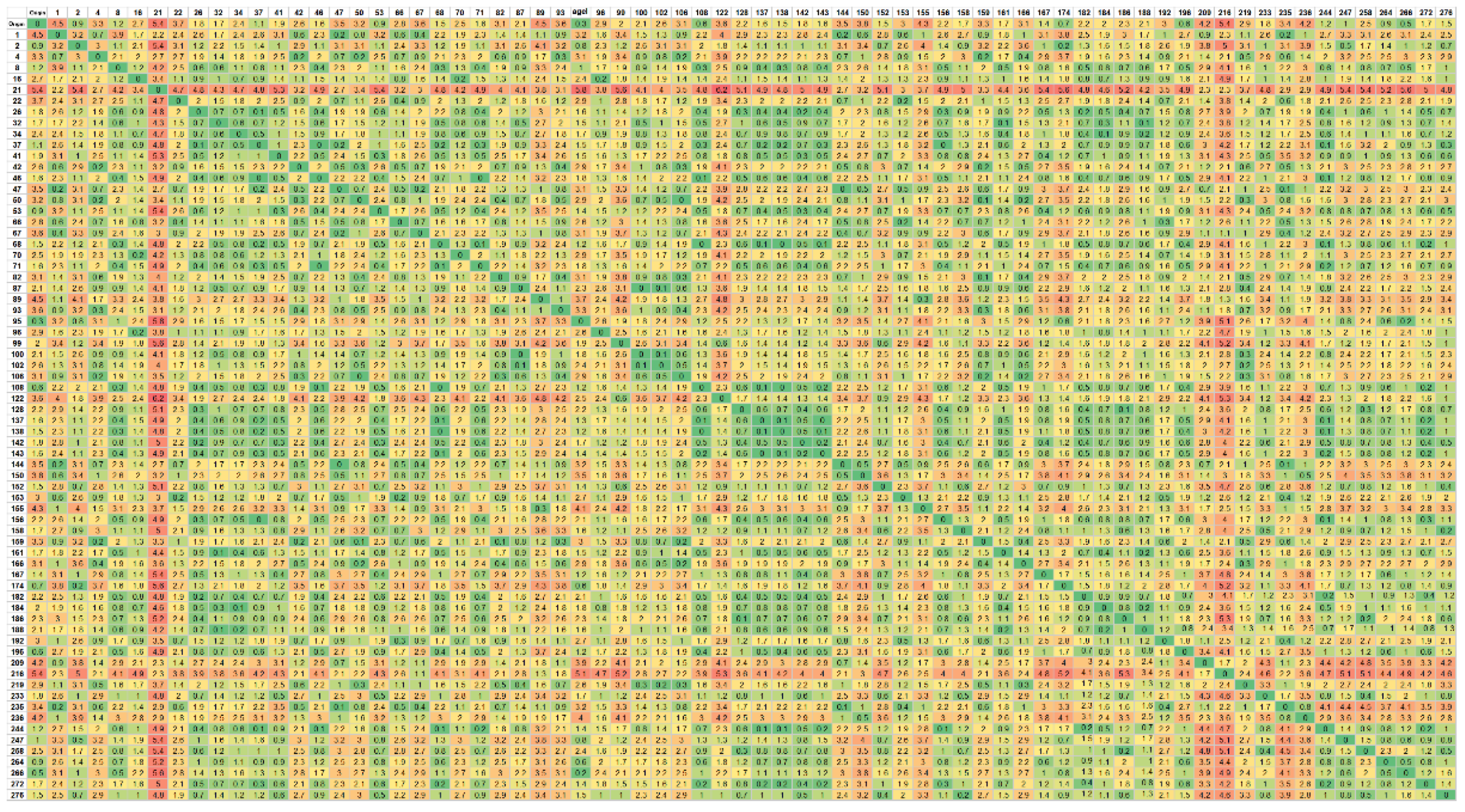
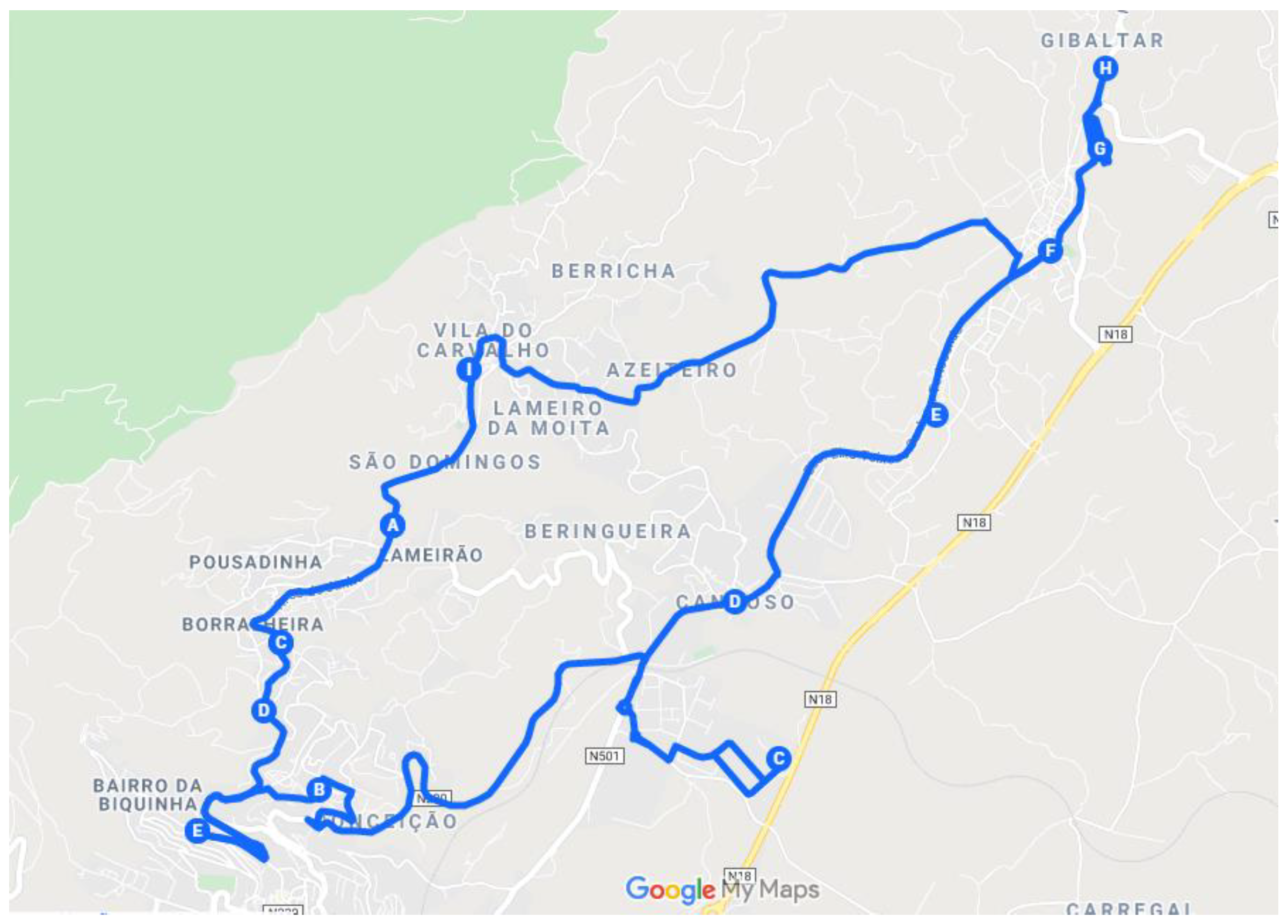
4.3. Central Zone

The zone defined as the Central Zone represents around 100 establishments. However, as some are in the same buildings or at a distance of less than 10 m (distance defined as the limit for considering clusters in this zone), some points were grouped together, thus reducing to 72 key points. These points can be seen in Figure 7.

As the distances between points are very small, there is no need to obtain an optimal solution as all points are close and relatively close to the Headquarters, within a radius of about 5 km. Thus, it was not necessary to carry out an equally detailed analysis of the 72 × 72 matrix, as it happened in the other zones. It was only necessary to run the algorithm for four salesmen, representing the two days of the week associated with the two workers. The 72 × 72 matrix can be seen in Figure 8.

5. Analysis of Results

5.1. North Zone

Figure 9 shows the route that covers all points in the North Zone, which served as the base for the analysis that led to the maximization of some distances. After applying the algorithm for two salesmen, the routes observed in Figure 10 and Figure 11 were returned.

Figure 10 represents the route that was referred to as the inside route, which runs through the points in the North Zone closest to the city.

In Figure 11, the route identified as the outside route is represented, which includes the remaining locations. As defined, this route already includes the key point 69 cluster.

Table 3. Routes optimization for the North zone.

Route	Key Points	Distance (km)
Long route	0→121→73→215→145→52→162→60→148→229→261→103→217→202→57→175→125→253→213→15→69→212→139→136→230→169→180→0	126.30
1st route	0→217→202→57→175→125→253→213→15→69→212→139→136→230→169→180→0	118.60
2nd route	0→121→60→162→148→229→261→103→52→145→215→73→0	21.10

shows the distances of the various routes mentioned above.

5.2. South Zone

Figure 12 shows the route that covers all points in the South zone, which, through its analysis, led to the maximization of some distances. After applying the algorithm for two salesmen, the routes observed in Figure 13 and Figure 14 were returned.

Once again, it is possible to conclude that the algorithm itself always opts for a larger route shown in Figure 13, and a smaller one shown in Figure 14, to minimize the distances from the first and last point of the routes to the origin.

In Figure 13 it is possible to observe the triangulation that occurs in the Paul-Casegas section. The distances between these points had to be maximized so that the algorithm would return the route that the worker will take.

In this particular case, it is beneficial that the road that connects Paul to Casegas (44) is traveled in both directions, although there is an alternative connection between 44 and 3 (Erada, the location that would be visited next, if the matrix was not adapted). The use of this route would result in a greater distance covered.

Figure 14 shows the route that runs through the establishments in the South zone of the city.

Comparing Figure 13 and Figure 14, it is possible to see that, when returning to the headquarters, the sellers will go through very close roads (top of the outside route and bottom of the inside route) that could even be visited in an alternative route that encompassed all these points. However, in order for daily routes to be balanced and sellers to cover roughly the same number of establishments per day, the minimum number of points to visit on each route has a significant impact on the distribution of points.

Table 4. Routes optimization for the South zone.

Route	Key Points	Distance (km)
Long route	0→260→54→218→259→254→199→120→131→79→44→220→101→105→126→133→75→118→18→208→86→267→59→214→83→243→270→0	119.65
1st route	0→260→54→214→218→259→254→199→120→131→79→44→220→101→105→126→133→0	100.50
2nd route	0→270→243→83→208→18→118→75→267→59→86→0	31.95

includes the distances of the various routes mentioned above.

5.3. Central Zone

For the Central zone of the city, four routes were generated: two for each worker, representing the two days of the week that will be assigned in this zone. These routes are shown in Figure 15a–d.

Thus, taking into account the proximity of all points, there was no need to optimize the routes, so the 72 × 72 matrix was considered (Figure 8). As can be seen in

Table 5. Routes optimization for the Central zone.

Route	Key Points	Distance (km)
1st route	0→196→161→188→16→42→4→50→159→93→82→106→166→219→102→87→100→32→8→266→95→0	8.24
2nd route	0→158→66→1→67→155→89→216→21→209→144→150→236→235→192→70→46→108→0	15.40
3rd route	0→264→167→41→142→26→184→34→182→244→156→272→68→138→137→143→2→174→0	5.99
4th route	0→53→71→128→186→258→233→122→99→152→96→22→153→47→37→276→247→0	9.03

, the distances of the routes within this zone have much smaller values than the other zones.

6. Discussion

The current algorithm allows for the best optimization to this kind of problem. The singularity of the orography in this case study requires special attention and the adaptability of the algorithm. The current adaptation to the algorithm proposed by Kirk [22] represents a versatile answer to the need for routing. Because of the simplicity of the inputs, some can easily be changed to accommodate the current needs of its user.

Given the inability to predict when changes will occur, punctual or definitive, in the number of workers, the flexibility of the developed tool represents a very important feature, as it allows for high adaptability to the day-to-day of the company in which it is applied.

The fact that the routes were previously divided in a way so that Fridays are reserved for unforeseen events and trips to establishments that, for some reason, were not visited, gives the company a larger margin, as the routes associated with the worker or workers missing can be carried out on that day. The solutions presented for the division of zones and places by days have a large scope for responding to unforeseen events, however, the possibility of changing routes was never excluded. This way, given the need for this change, it is only necessary to change the parameter referring to the number of available workers, thus allowing a new route solution to be returned, adapted to the new problem, for the whole week or just for a specific day. Other parameters, like the minimum number of visited establishments and the matrix size, can be changed in order to obtain different solutions, only needing to adapt the distances’ matrix accordingly to the weekly needs.

Considering the optimizations proposed in this article, the total sum of distances traveled would decrease to 309 km per week for sellers, and these routes would be replicated by distributors, for a total of 618 km per week. Although the shorter intra-cluster distances were not considered in this study, as they are relatively short distances and often end up not being actually covered, a decrease of more than half of the covered kilometers by the workers is expected. This significant reduction was possible due to adjustments made in the functions of workers in the company and through the application of the m-TSP resolution algorithm [22] with some adaptations in the distance matrices. Despite the good results obtained, it is important to highlight the limitations characteristic of this type of problem. This type of algorithm does not consider constraints, such as traffic, orography of the area, road directions and, perhaps most significantly, does not take into account the possibility of visiting a path and returning by the same route if distances so justify because it is based on the m-TSP approach. This limitation leads to the need of adapting the distance’s matrix for each zone, preventing the choice of certain roads, which the users may know are not reliable.

7. Conclusions

Given the lack of algorithm and methods applicable to this case study in particular, due to the orography, an adapted Genetic Algorithm was applied to the Multiple Traveling Salesman Problem (m-TSP) as a decision support system for optimizing a beverage logistics vehicle routing problem. A case study was developed in a mountain region city, Covilhã (Portugal) to optimize routes, for the five days of the week, which minimize travel costs and the distances traveled by workers, considering the approximately 270 establishments. The optimization of the daily routes for the workers assigned to distribution was divided into three zones: North, South and Central. A reduction of 618 km per week of the total distance traveled was determined by the algorithm. This result promotes provider-client relations by ensuring that clients are visited in time; reduces the fixed costs with fuel by the lower distance traveled and simultaneously promotes environmental sustainability by the shortening of logistical routes. All these improvements and optimizations can be thought of as contributions to foster smart cities.