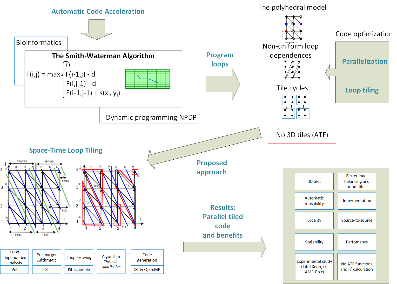
Space-Time Loop Tiling for Dynamic Programming Codes

Abstract

We present a new space-time loop tiling approach and demonstrate its application for the generation of parallel tiled code of enhanced locality for three dynamic programming algorithms. The technique envisages that, for each loop nest statement, sub-spaces are first generated so that the intersection of them results in space tiles. Space tiles can be enumerated in lexicographical order or in parallel by using the wave-front technique. Then, within each space tile, time slices are formed, which are enumerated in lexicographical order. Target tiles are represented with multiple time slices within each space tile. We explain the basic idea of space-time loop tiling and then illustrate it by means of an example. Then, we present a formal algorithm and prove its correctness. The algorithm is implemented in the publicly available TRACO compiler. Experimental results demonstrate that parallel codes generated by means of the presented approach outperform closely related manually generated ones or those generated by using affine transformations. The main advantage of code generated by means of the presented approach is its enhanced locality due to splitting each larger space tile into multiple smaller tiles represented with time slices.

1. Introduction

In this paper, we deal with the generation of parallel tiled code for dynamic programming codes.

Increasing dynamic programming code performance is not a trivial problem because, in general, that code exposes affine non-uniform data dependence patterns typical for nonserial polyadic dynamic programming (NPDP) [1], preventing tiling the innermost loop in a loop nest that restricts code locality improvement. There are many state-of-the-art manual transformations for DP algorithms [2,3,4,5] and dedicated software [6,7,8]. The inherent disadvantage of those solutions is that they were developed for specific dynamic programming tasks. Thus, in general, they cannot be applied to an arbitrary DP algorithm. In addition to that, a manual parallel code development may be very costly.

Fortunately, dependence patterns of NPDP code can be represented with the polyhedral model [9]. Thus, well-known polyhedral techniques and corresponding compilers can be applied to automatically tile and can parallelize such a code, for example, the PLuTo and PPCG academic compilers as well as the commercial R-STREAM and IBM-XL compilers. They extract and apply affine transformations to tile and parallelize loop nests. They have demonstrated considerable success in generating high-performance parallel tiled code, in particular, for uniform loop nests.

However, optimizing loop nests, which exposes affine non-uniform dependences typical for dynamic programming codes, by means of affine transformations is not always possible or fruitful: tiling or parallelization is not possible, only some loops (not all loops) in a nest can be tiled, or the generated parallel code is not scalable [10,11,12].

In order to increase code locality and generate coarse-grained code, loop tiling [13,14,15,16,17,18,19] can be applied. Tiling for improving locality groups loop statement instances into smaller blocks (tiles) allows reusability when the block fits into local memory. In parallel tiled code, tiles are considered as indivisible macro statements each executed with a single thread that increases code coarseness.

PLuTo [13] is the most popular state-of-the-art, source-to-source polyhedral compiler that automatically generates parallel tiled code.

Unfortunately, PLuTo fails to tile all loops in a given loop nest in the case of DP programs exposing non-uniform dependences [10]. This reduces the locality of target tiled code.

The idea of tiling presented in our previous paper [10] is to transform (correct) original rectangular tiles so that all target tiles are valid under lexicographical order. Tile correction is performed by the transitive closure to loop nest dependence graphs. However, the correction technique can generate irregular tiles, and some of them can be too large [20]. Those drawbacks do not allow us to achieve maximal code locality and performance [21].

In this paper, we present a new approach, which enables us to generate parallel tiled code of enhanced locality for a broad class of dynamic programming codes. Experimental results demonstrate that the code generated by means of the presented approach outperforms closely related ones.

The approach presented in this paper can be applied to any affine loop nest, but its effectiveness is empirically confirmed by us only for a class of dynamic programming codes that expose affine non-uniform dependences for which its features prevent tiling one or more the innermost loops in a loop nest. Papers [11,12] affirm that achieving peak performance for dynamic programming codes requires tiling all loops (including the innermost one) when the full dynamic programming matrix is significantly larger than the cache size. We also empirically discovered that tiling the innermost loop is very important for improving code locality for dynamic programming codes [21].

Thus, currently we limit the proposed approach only to dynamic programming codes exposing dependences preventing tiling the innermost loop. Adapting the approach for resolving other problems is a topic for future research.

2. Background

In this paper, we deal with generation of parallel tiled code for the three dynamic programming codes implementing the Smith–Waterman (SW) algorithm, the counting algorithm, and the Knuth optimal binary search tree (OBST) algorithm.

The Smith–Waterman algorithm explores all the possible alignments between two sequences, and it returns the optimal local alignment guarantying the maximal sensitivity as a result [22].

It constructs a scoring matrix, H, which is used to keep track of the degree of similarity between the cells $a_i$ and $b_j$ of two sequences to be aligned, where $1\le i\le N,1\le j\le M$. The size of the scoring matrix is (N+1)*(M+1). Matrix H is first initialized with $H_{0,0}=H_{0,j}=H_{i,0}=0$ for all i and j.

The next step is filling matrix H. Each element $H_{i,j}$ of H is calculated as follows:

$$H_{i,j}=max\left\{\begin{array}{c}{H}_{i-1,j-1}+s(a_i,b_j)\hfill \\ \underset{1\le k<i}{max}(H_{i-k,j}-W_k)\hfill \\ \underset{1\le k<j}{max}(H_{i,j-k}-W_k)\hfill \\ 0\hfill \end{array}\right.,$$

where $s(a_i,b_j)$ is a similarity score of elements $a_i$ and $b_j$ that constitute the two sequences, and $W_k$ is a penalty of a gap that has length k.

The final step of the SW algorithm is trace back, which generates the best local alignment. The step starts at the cell with the highest score in matrix H and continues up to the cell, where the score falls down to zero.

The SW algorithm is $\mathcal{O}$(MN(M + N)) in time and $\mathcal{O}$(MN) in memory. The extra time factor of (M + N) comes from finding optimal k by looking back over entire rows and columns.

The loop nest implementing the SW algorithm is presented in Listing 1.

Listing 1. Calculating scoring matrix H using the SW algorithm.

for (i=1; i <=N; i++)  for (j=1; j <=M; j++)  {   for (k=1; k <=i; k++)     m1[i][j] = max(m1[i][j], H[i-k][j] - W[k]); //s0   for (k=1; k <=j; k++)     m2[i][j] = max(m2[i][j], H[i][j-k] - W[k]); //s1    H[i][j] = max(0,H[i-1,j-1]+ s(a[i],b[i]), m1[i][j], m2[i][j]);  //s2  }

Listing 1. Calculating scoring matrix H using the SW algorithm.

for (i=1; i <=N; i++)  for (j=1; j <=M; j++)  {   for (k=1; k <=i; k++)     m1[i][j] = max(m1[i][j], H[i-k][j] - W[k]); //s0   for (k=1; k <=j; k++)     m2[i][j] = max(m2[i][j], H[i][j-k] - W[k]); //s1    H[i][j] = max(0,H[i-1,j-1]+ s(a[i],b[i]), m1[i][j], m2[i][j]);  //s2  }

The counting algorithm computes the exact number of nested structures for a given RNA sequence. It was also introduced by Michael S. Waterman and Temple F. Smith [23]. The authors applied NPDP and tabularized results for subproblems. The approach populates the matrix C with the following recursion:

$$\begin{array}{c}\hfill C_{i,j}=C_{i,j-1}+{\sum }_{\genfrac{}{}{0pt}{}{i\le k<(j-l)}{S_k,S_j\mathrm{pair}}}{C}_{i,k-1}·C_{k+1,j-1},\end{array}$$

where n is the sequence’s S length, l is the minimal number of enclosed positions, and the entry $C_{i,j}$ provides the exact number of admissible structures for the subsequence from position i to j. The upper right corner $C_{1,n}$ presents the overall number of admissible structures for the sequences.

The code implementing the counting algorithm is presented with Listing 2.

Listing 2. Populating matrix C using the Counting algorithm.

for (i = N-1;  i>=0; i--){  for ( j=i+1; j<= N; j++){    for ( k = i; k<=j-l; k++){      c[i][j] +=  c[i][j-1] + paired(k,j) ?  c[i][k-1] + c[k+1][j-1] : 0;    }  } }

Listing 2. Populating matrix C using the Counting algorithm.

for (i = N-1;  i>=0; i--){  for ( j=i+1; j<= N; j++){    for ( k = i; k<=j-l; k++){      c[i][j] +=  c[i][j-1] + paired(k,j) ?  c[i][k-1] + c[k+1][j-1] : 0;    }  } }

The third NPDP benchmark that we consider in this paper is the optimal binary search tree (OBST) [24], which is the case when the tree cannot be modified after it has been constructed.

Knuth’s OBST algorithm populates matrix C and is represented with the following recurrence:

$$C_{i,j}=min\left\{\begin{array}{c}{C}_{i,j}\hfill \\ \underset{1\le i<k<j\le n}{min}(C_{i,k}+C_{k,j}+W_{i,j}),\hfill \end{array}\right.$$

where $W(i,j)$ is the sum of the probabilities that each of the items i through j will be accessed.

The recurrence can be implemented with the triple nested loops presented in Listing 3.

Listing 3. Populating matrix C using the Knuth algorithm.

for (i=n-1; i >=1; i--)   for (j = i+1; j <= n ; j += 1)     for (k = i+1; k <j; k += 1) {       c[i][j]= min(c[i][j], w[i][j]+c[i][k]+c[k][j]);     }

Listing 3. Populating matrix C using the Knuth algorithm.

for (i=n-1; i >=1; i--)   for (j = i+1; j <= n ; j += 1)     for (k = i+1; k <j; k += 1) {       c[i][j]= min(c[i][j], w[i][j]+c[i][k]+c[k][j]);     }

All the three loop nests above are within the class of affine loops, i.e., for given loop indices, lower and upper bounds, as well as array subscripts and conditionals, are affine functions of surrounding loop indices and possibly of structure parameters (defining loop index bounds), and the loop steps are known constants.

Thus, the affine transformation framework [16,25] can be applied to each of those loop nests in order to generate parallel tiled code manually or automatically. However, for each of them, affine transformations do not exist that would allow for tiling the innermost loop. This considerably reduces target code locality.

Perfectly nested loops are ones wherein all statements are comprised in the innermost loop, otherwise the loops are arbitrarily nested.

Given a loop nest with q statements, its polyhedral representation includes the following: an iteration space $I{S}_i$ for each statement $S_i,i=1,\dots ,q$, read/write access relations ($\mathit{RA}$/$\mathit{WA}$, respectively), and global schedule S corresponding to the original execution order of statement instances in the loop nest.

The loop nest iteration space $I{S}_i$ is the set of statement instances executed by a loop nest for statement $S_i$. An access relation maps an iteration vector $I_i$ to one or more memory locations of array elements. Schedule S is represented with a relation, which maps an iteration vector of a statement to a corresponding multidimensional timestamp, i.e., a discrete time when the statement instance has to be executed.

The algorithms presented in this paper use a dependence relation that is a tuple relation of the form $\left\{\right[inputlist]\to [output\mathrm{list}\left]\right|formula\}$, where input list and output list are the lists of expressions used to describe input and output tuples, and formula describes the constraints imposed upon input and output lists. It is a Presburger formula built of constraints represented by algebraic expressions and uses logical and existential operators.

In the presented algorithm, standard operations on relations and sets are used, such as intersection (∩), union (∪), and application of relation R on set S: $R\left(S\right)=\{\left[e^{\prime }\right]\mid \exists e\in S\wedge \left[e\right]\to \left[e^{\prime }\right]\in R\}$, i.e., this operation results in a set for which its tuple $e^{\prime }$ is the output tuple of relations $R^{\prime }\in R$ in which its input tuple e belongs to set S.

A global (original) schedule is a relation that maps an iteration vector of a statement to a unique multidimensional discrete time. Such a schedule presents the lexicographic order of loop nest statement instances in the global (common) iteration space. In order to extract a global schedule, we apply the PET tool [26].

3. Overview of Space-Time Tiling

For a given loop nest, optimizing compilers based on affine transformations such as PLuTo to generate tiles for which its dimension is equal to the number of linear independent solutions to the time partition constraints formed for that nest [16]. If this number is less than the loop nest depth defined with the number of loops in a nest, the target tiles are unbounded for loops with parametric (unbounded) upper bounds.

For example, if, for a loop nest of depth three in which its loop indexes are $i,j$ and k, there exist only two linearly independent solutions to the time partition constraints formed for that loop, we are able to form only two-dimensional tiles $m\times n$, where m and n are the sizes of a tile along loop indices i and j, respectively. Let two new outer loops $ii$ and $jj$ be responsible for enumerating tiles in the target code. Then, in that code for given values of $ii$ and $jj$, the three inner loops $i,j$ and k enumerate statement instances within a hypercube in which its sides are bounded along axes i and j with values of m and n, but the size along axis k is not limited. This is equivalent to the fact that each target tile is unbounded (parametric) when the upper bound of k is a parameter. As a result, for large size problems, all the data associated with such an unbounded tile cannot be held in a cache that reduces code locality.

In order to increase code locality, we propose to split each unbounded target space tile into smaller ones. Such a splitting is based on forming time slices. A time slice is a set of statement instances belonging to one or more the same time partitions. Statement instances within a time partition have the same multidimensional execution time. Time slices can be formed by means of any valid statement instance schedule.

As a result, we increase the target tile dimension by one. That additional dimension is implemented with an additional loop in the target tiled code. It enumerates time partitions—smaller tiles—within a larger tile. As our experiments demonstrate, for dynamic programming codes, this improves code locality, which results in improving parallel-tiled code performance.

The following section presents details how the presented above idea of space-time tiling can be realized.

4. Space-Time Tiling

In this section, we first illustrate space-time tiling by means of a simple loop nest; Then, we demonstrate how it can be adapted to arbitrarily nested loops, discuss how parallel tiled code can be generated, and finally present a formal algorithm.

4.1. Tiling a Simple Loop Nest

Let us consider the following loop nest.

Example 1.

  for(i = 1; i <= n; ++i)

    for(j = 1; j <= n; ++j)

      A[i][j] = A[i-1][j+1]+A[i][j-1];

The relation below represents dependences available in the loop nest above:

$$R:=\bigcup \left\{\begin{array}{c}\left[n\right]\to \left\{\right[i,j]\to [i,1+j]\mid 0<i\le n\wedge 0<j<n\}\hfill \\ \to \left\{\right[i,j]\to [1+i,-1+j]\mid 0<i<n\wedge 2\le j\le n\}\hfill \end{array}\right.,$$

where “$\left[n\right]\to$” means that n is the parameter; $[i,j]$, $[i,1+j]$, and $[1+i,-1+j]$ are the relation tuples; $0<i\le n\wedge 0<j<n$ and $0<i<n\wedge 2\le j\le n$ are the affine relation constraints; ∧ is the conjuction operator of affine constraints; and ∪ is the union operator of relations.

Figure 1a shows dependences (black arrows) for the loop nest when $n=4$. We split the entire iteration space into two subspaces, each of width two (in general, any width can be chosen). A parametric set, $SPACE$, below represents those sub-spaces:

$$SPACE:=[n,id\_sp]\to \left\{\right[i,j]\mid i>2id\_sp\wedge 0<i\le 2+2id\_sp\wedge i\le n\wedge 0<j\le n\},$$

where parameter $id\_sp$ is the identifier of a sub-space. For each particular value of parameter $id\_sp$, we obtain a specific set representing the corresponding sub-space.

In Figure 1a, the black vertical line divides the entire iteration space into two subspaces, $SPACE0$ and $SPACE1$, defined with parameters $id\_sp=0$ and $id\_sp=1$, respectively.

Let $IS$ be the loop nest iteration space. Then, we form a valid affine schedule for loop nest iterations by applying the “m3: = schedule IS respecting m1 minimizing m2” operator of the iscc calculator [27], which computes a schedule for loop nest iteration space $IS$ that respects all dependences in relation $m1$ and tries to minimize the dependences in relation $m2$. As $m1$ and $m2$, we take relation R and obtain the following schedule in the tree form [28]:

domain: "[n] -> { [i, j] : 0 < i <= n and 0 < j <= n and ((i < n and j >= 2) or

                (i >= 2 and j < n) or j >= 2 or j < n) }"

  schedule: "[n] -> [{ [i, j] -> [(i)] }, { [i, j] -> [(i + j)] }]"

where the lines beginning with the word domain represent the iteration domain where the schedule returned for the considered loop nest is valid. The lines beginning with the word schedule represent the two different schedules for the loop nest of Example 1, i.e., $[i,j]->\left[\right(i\left)\right]$ and $[i,j]->\left[\right(i+j\left)\right]$, which means that iteration $[i,j]$ is mapped to times $\left[\right(i\left)\right]$ and $\left[\right(i+j\left)\right]$, respectively.

In order to form a relation implementing wave-fronting [29], we calculated the sum of the two schedules above: i and $i+j$ that results in the expression $2i+j$, which allows for statement instance parallelization [29]. We present a target schedule with relation, $SCHED$, which maps each loop nest statement instance to a time partition, as follows:

$$SCHED:=\left[n\right]\to \left\{\right[i,j]\to [2i+j\left]\right\}\cap IS,$$

where $IS$ is the loop nest iteration space, and ∩ is the operator of the intersection of the domain of the relation $SCHED:=\left[n\right]\to \left\{\right[i,j]\to [2i+j\left]\right\}$ with $IS$.

Iterations defined with vector ${(i,j)}^T$ and belonging to the same schedule time $(2i+j)$ can be executed in parallel, for example, iterations (1, 3) and (2,1).

Figure 1a presents ten time partitions shown with blue lines ($t0,t1,\dots ,t9$). Using those partitions, we form parametric time slices, each including the same number of time partitions. Supposing that each time slice includes three time partitions (in general, an arbitrary number of time partitions can be included in a single time slice), we obtain the following formula for set, $TIME$, representing time slices:

$$TIME:=[n,id\_t]\to \left\{\right[i,j]\mid 3id\_t+3\le 2i+j\le 3·(id\_t+1)+2\}\cap IS,$$

where $id\_t$ is the parameter defining the identifier of a time slice. The value of parameter $id\_t$ defines a specific time slice, for example, for $n=4$ and $id\_t=0$, we obtain the following set.

$$TIME:=\left\{\right(1,1);(1,2);(1,3);(2,1\left)\right\}.$$

Let us note that the size of sub-spaces represented with set $SPACE$ is unbounded (parametric) for a parametric loop nest. Using such subspaces as tiles can reduce code locality when the size of the data associated with a subspace is greater than cache size. To improve code locality, we intersected subspaces represented with set $SPACE$ with time slices described with set $TIME$. This causes the splitting of each sub-space into smaller target tiles, which allows us to improve code locality.

Thus, we calculate a parametric set, $TILE$, defining target tiles as follows.

$$TILE:=TIME\cap SPACE.$$

For the considered example, this set is the following.

$$\begin{array}{c}\hfill TILE:=[n,id\_sp,id\_t]\to \left\{\right[i,j]\mid i>2id\_sp\wedge 0<i\le 2+2id\_sp\wedge i\le n\wedge \\ \hfill j\ge 3+3id\_t-2i\wedge 0<j\le 5+3id\_t-2i\wedge j\le n\wedge \\ \hfill (j\ge 2\vee (i\ge 2\wedge j<n)\vee (i<n\wedge j\ge 2)\vee j<n)\}.\end{array}$$

An identifier of each tile is represented with a pair of parameters $id\_sp$ and $id\_t$. Tiles represented with set $TILE$ for $n=4$ are shown in Figure 1b with red figures. For example, the tile for which its identifier is 01 ($id\_sp=0,id\_t=1$) includes the following iterations: (1,4), (2,2), (2,3), and (2,4).

Enumerating obtained tiles in lexicographical order is valid because all elements of distance vectors of inter-tile dependeces are non-negative. To prove this fact, it is enough to perceive that, for subspaces represented with set $SPACE$, there exist only forward dependence directions (no backward dependence directions). Thus, dependences between subspaces spread from ones with smaller values of parameter $id\_sp$ to those with greater ones. This prevents any cycle among subspaces. We make the same conclusion regarding to time slices represented with parameter $id\_t$: Dependences between them spread only in the forward direction. Thus, all elements of distance vectors of inter-tile dependences are non-negative.

In order to generate target code, we first form relation, $CODE$, using set $TILE$ as follows.

$$CODE:=\left[n\right]->\left\{\right[i,j]\to [id\_sp,id\_t,i,j\left]\right\}\cap IS.$$

That relation maps each iteration $[i,j]$ within the iteration space $IS$ to the tuple $id\_sp,id\_t,i,j$, which represents the tile identifier $[id\_sp,id\_t]$ and the iteration itself $[i,j]$. Then, we apply the iscc codegen operator to relation $CODE$ in order to obtain the following pseudo-code.

for(c0=0; c0 < (n+1)/2; c0++)

 for(c1=c0+c0/3; c1<=c0+(n+c0+1)/3; c1++)

  for(c2=max(2*c0+1, c1-n+(n + c1)/2 +2);

       c2 <= min(min(n, 2*c0 + 2), c1 + c1/2 + 2); c2++)

   for (c3 = max(1, 3 * c1 - 2 * c2 + 3); c3 <= min(n, 3*c1-2*c2 + 5); c3++)

      (c0, c1, c2, c3);

The first two outer loops of that code enumerate values of parameters $id\_sp$ and $id\_t$, while the reminding inner two loops scan iterations within a tile defined with values of those parameters.

4.2. Imperfectly Nested Loops

For imperfectly nested loops, each statement has a local iteration space. In general, iteration spaces of distinct statements can be of different dimensions. Thus, it is not possible to directly calculate distance vectors of dependences for which sources and destinations originated with instances of different statements. To cope with this problem, we formed a global iteration space common to instances of all statements. Let us remind the reader that a global schedule presents the original (serial) execution order of each loop nest statement in an iteration space common (global) to all statements. Thus, we apply a global schedule on each named tuple of a dependence relation (see the description of the relation application operator on a set in Section 2). For this purpose, we apply the iscc operator apply map m to set s, where m is the relation representing global schedule, s is a particular tuple of the dependence relation. This results in a new dependence relation for which its tuples are unnamed and of the same size; it describes dependences in a global (common) iteration space for all loop nest statement instances.

Distance vectors can be calculated as the difference between the image and domain of that new relation (representing dependences in the global iteration space) by means of the iscc deltas operator. This is possible because the image and domain of that relation are represented with affine sets for which its tuples have the same dimensions.

In general, for affine dependences, obtained distance vectors may not include only integer element values, and their elements can be represented with affine expressions. Thus, calculated distance vectors have the following meaning: They represent all the possible distances between the source and destination of each dependence available in a given loop nest in the global iteration space. In general, for affine dependences, the number of such distances can be unlimited (parametric).

Next we convert those vectors to a single direction vector, which characterizes the directions of all distance vectors. Each element of this vector holds “+” (“−”) if the corresponding element in all distance vectors is non-negative (at least one element is negative). It is worth noting that, in general, the length of a distance vector can be larger than that of a direction vector because a distance vector can include additional constants inserted in tuples of a global schedule. However, all distance vectors in the global (common) iteration space are of the same length, and the constants inserted are in the same positions for all vectors.

Throughout the whole paper, we use the following notations: $I_i$ is the iteration vector of the iteration space of statement $Si$, $PARAM{S}_i$ denotes the structure parameters of the loops surrounding statement $Si$, $I{S}_i$ is the iteration space of statement $S_i$, $S_i\left[I_i\right]$ is the named tuple representing the iteration vector $I_i$ of statement $S_i$, and $T_i\left(I_i\right)$ is the global (original) schedule time of iteration $I_i$ of statement $S_i$.

To form a direction vector, which symbolizes all dependence vectors available in a given loop nest, we apply Procedure 1 below, which takes into account that the first element of each distance vector is non-negative (negative) if the corresponding loop iterator is incremented (decremented).

Procedure 1. Calculation of a common direction vector.

Input: Relation, R, describing all the dependences available in a loop nest, global schedule

$SCHED\_GLO{B}_i:=\left[PARAM{S}_i\right]\to \{S_i\left[I_i\right]\to \left[T_i\left(I_i\right)\right]\}$ for each of q statements $\mathrm{S}i,i=1,2,\dots ,q$; the length of an iteration vector in the global iteration space, n; the loop nest depth, d, $d\le n$.

Output: A common direction vector.

Method:

• Form relation $R^{\prime }$, representing dependences in the global iteration space, by means of replacing each named tuple, $S_i\left[I_i\right]$, of relation R with the tuple resulting due to relation $SCHED\_GLO{B}_i$ on tuple $S_i\left[I_i\right]$;
• Apply the $deltas$ operator of the iscc calculator to relation $R^{\prime }$ to calculate distance vectors in the common iteration space.
• Initialize a common direction vector of length d, $DIR\_VEC$, as follows;
  $DIR\_VECT={(+,+,\dots +)}^T$, $k=2$, $j=2$.
• $L1:$ If the j-th element of the distance vectors is a global schedule constant, say c, then if $c\ge 0$$j=j+1$, proceed to $L2:$; or else $DIR\_VECT\left(k\right)$= “-”, $k=k+1,j=j+2$, proceed to $L2$.
  If the j-th element of at least one distance vector is negative (positive) and the corresponding iterator is incremented (decremented), then
  $DIR\_VECT\left(k\right)$= “-”, $k=k+1,j=j+1$;
  $L2:$ If $j⩽n$, proceed to $L1$; otherwise return vector $DIR\_VECT$, the end.

Let us consider the following example of the distance vector:

$\left[N\right]\to \left\{\right[i0,i0,1,i3]\mid 0\le i0\le 1\wedge 2-N+2i0\le i3\le 0\},$

where “1” in the third position of the vector is the global schedule constant.

For that example, Procedure 1 returns the following common direction vector.

$$DIR\_VEC={(+,+,-)}^T.$$

Using vector $DIR\_VEC$, we apply Procedure 2 below to form sets $SPAC{E}_j$, $j=l_1,l_2,\dots ,l_m$, where $l_1,l_2,\dots ,l_m$, are the positions of non-negative elements of vector $DIR\_VEC$, m is the number of non-negative elements within vector $DIR\_VEC$. Those sets define rectangular subspaces of given width $b_j$ along axis j.

Procedure 2. Calculation of sets $SPAC{E}_j$ defining rectangular subspaces of given width $b_j$ along axis j.

Input: A common direction vector $DIR\_VEC$ of length d returned with Procedure 1; variables $b_k,k=1,2,\dots ,d$, defining the width of a sub-space along axis $i_k$; lower $l{b}_k$ and upper $u{b}_k$ bounds of loop iterator $i_k,k=1,2,\dots ,d$; the number of the statements in the loop nest, q.

Output: Sets $SPAC{E}_j,j=l_1,l_2,\dots ,l_m$; values of variables $l_1,l_2,\dots ,l_m$.

Method:

• $j=1;k=1$;
• If $DIR\_VEC\left(j\right)$== “+”, then form the following sets
  $SPAC{E}_j^i:=\left[PARAM{S}_i,i{i}_j\right]\to \{S_i\left[I_i\right]\mid b_j\ast i{i}_j+l{b}_j\le i_j\le$
  $\min \left(b_j\ast \left(i{i}_j+1\right)+l{b}_j-1,u{b}_j\right)\wedge i{i}_j\ge 0\}\cap I{S}_i,i=1,2,\dots ,q$;
  $l_k=j$; $k=k+1$;
• $j=j+1$; if $j\le d$ then proceed to step 2;
• Form set $SPAC{E}_j$ as follows;
  $SPAC{E}_j:={\sum }_{i=1}^{q}SPAC{E}_j^i,j=l_1,l_2,\dots ,l_m$.

For each of q loop nest statements, we form a valid schedule respecting all the dependences represented with relation R and allowing for wavefronting of any well-known technique, for example [28], and present it as the following relation:

$$SCHE{D}_i:=\left[PARAM{S}_i\right]\to \{S_i\left[I_i\right]\to [t_1,t_2,\dots ,t_{k_i}]\}\cap I{S}_i,i=1,2,\dots ,q,$$

where tuple $[t_1,t_2,\dots ,t_{k_i}]$ represents the $k_i$-dimensional schedule for instances of statement $S_i$.

If a schedule allowing for wave-fronting cannot be formed (a scheduler returns only one schedule for each loop nest statement), then we skip the steps aimed at forming time slices.

In general, relation $SCHE{D}_i$ maps each instance of statement $S_i$ to a discrete multidimensional time. A set of statement instances belonging to the same multidimensional time defines a time partition. Time partitions are represented with the inverse relation, $SCHE{D}_i^{-1}$, of relation $SCHE{D}_i$.

$SCHE{D}_i^{-1}:=\left[PARAM{S}_i\right]\to \{[t_1,t_2,\dots ,t_{k_i}]\to S_i\left[I_i\right]\}\cap I{S}_i$, $i=1,2,\dots ,q$.

For each of q loop nest statements, using relation $SCHE{D}_i^{-1}$, we form set $TIM{E}_i$ defining time slices each including a constant number of time partitions:

$$\begin{array}{c}\hfill TIM{E}_i:=[PARAM{S}_i,t_1,t_2,\dots ,t_{k_i-1},id\_t]\to \\ \hfill \left\{S_i\left[I_i\right]\right|\exists t_{k_i}s.t.n\_t\ast id\_t<=t_{k_i}<=n\_t\ast (id\_t+1)-1\wedge \\ \hfill constraints\mathit{of}relationSCHE{D}_i^{-1}\}\cap I{S}_i,i=1,2,\dots ,q,\end{array}$$

where $t_{k_i}$ is the $k_i$-th dimension of schedule $SCHE{D}_i$; parameters $t_1,t_2,\dots ,t_{k_i-1},$$id\_t$ define the identifier of a time slice; and $n\_t$ determines the number of time partitions within a time slice.

Constant $n\_t$ is responsible for defining the number of time partitions within the time slice for which its identifier is $(t_1,t_2,\dots ,t_{k_i-1},$${id\_t)}^T$, i.e., for a given i, the inequality $n\_t\ast id\_t<=t_{k_i}<=n\_t\ast (id\_t+1)-1$ describes the interval in which the value of $t_{k_i}$ changes. The number of the values of that interval equals the number of the time partitions within a time slice. The choice of a one-dimensional schedule ($t_{k_i}$) in relation $SCHE{D}_i$ for defining the number of time partitions within a time slice is justified with practical observation. Such a choice is enough to form time slices for which its size is satisfactory in practice. Experiments with loop nests presented in Section 6 confirm that such a choice allows defining a large enough number of time partitions within a single time slice, which results in acceptable tiled code performance.

The formula to calculate sets, $TIL{E}_i$, for each statement $Si,i=1,2,\dots ,q,$ representing target tiles is the following:

$$TIL{E}_i:=TIM{E}_i\cap \bigcap _{j=l_m}^{l_1}SPAC{E}_j,i=1,2,\dots ,q,$$

where $l_1,l_2,\dots ,l_m$ are the positions of m non-negative elements of vector $DIR\_VEC$.

Let us note that the intersection ${\bigcap }_{j=l_m}^{l_1}SPAC{E}_j$ results in rectangular tiles for each statement $i=1,2,\dots ,q$. In general, the sizes of those tiles can be unbounded (parametric) when the number of non-negative elements of vector $DIR\_VEC$ is less than the number of loop nest iterators (loops). Using such tiles can reduce code locality when the size of the data associated with a rectangular tile is greater than cache size. In order to improve code locality, for each statement $i=1,2,\dots ,q$, we intersect the rectangular tiles with time slices represented with set $TIM{E}_i$. This causes splitting of each rectangular tile into smaller target tiles, which allows us to improve code locality.

It is worth noting that the dimension of tiles obtained with the intersection of rectangular tiles with time slices represented with set $TIM{E}_i$ is one more than the dimension of rectangular slices obtained as the intersection ${\bigcap }_{j=l_m}^{l_1}SPAC{E}_j$, $i=1,2,\dots ,q$. The intersection of rectangular tiles with time slices represented with set $TIM{E}_i$ is the basic idea of the approach proposed in this paper.

The identifiers of tiles are represented with the following vector:

$$TILE\_ID={(i{i}_{l_1},i{i}_{l_2},\dots ,i{i}_{l_m},t_1,t_2,\dots ,id\_t)}^T,$$

which can be re-written as stated below:

$$TILE\_ID={(I{D}_{space},I{D}_{time})}^T,$$

where $I{D}_{space}={(i{i}_{l_1},i{i}_{l_2},\dots ,i{i}_{l_m})}^T$, $I{D}_{time}={(t_1,t_2,\dots ,id\_t)}^T$.

Identifier $I{D}_{space}$ defines a sub-space being the intersection of sub-spaces $SPAC{E}_j,j=l_1,l_2,\dots ,l_m$. Since dependences among subspaces along axis $j=l_1,l_2,\dots ,l_m$ are spread only in the forward direction (due to the fact that the corresponding elements of the common direction vector are positive), all the corresponding dependence distance vectors regarding vector $I{D}_{space}$ have only non-negative elements. Thus, enumerating tiles regarding vector $I{D}_{space}$ in lexicographical order is valid.

Within each subspace represented with identifier $I{D}_{space}$, enumerating time slices defined with identifier $I{D}_{time}$ in lexicographic order is also valid because dependences along time slices spread from a slice with a lexicographically smaller identifier to those with larger ones. Thus, enumerating tiles where its identifiers are represented with vector $TILE\_ID$ in lexicographic order is valid.

It is worth noting that dependence distance vector $I{D}_{time}$ can have negative elements, with the exception of those from the first one ($t_1$). For example, for instances of some statement, two multidimensional schedules ${(2,1,1)}^T$ and ${(1,2,2)}^T$ can be valid. Thus, for that case $I{D}_{time}={(1,-1,-1)}^T$.

In order to generate serial code enumerating tiles in lexicographical order, we transform each set $TIL{E}_i$ to relation $COD{E}_i,i=1,2,\dots ,q$ of the following form:

$$\begin{array}{c}\hfill COD{E}_i:=\left[PARAM{S}_i\right]\to \{\left[I_i\right]\to [TILE\_ID,T_i\left(I_i\right)]|\\ \hfill constraint{s}_{i}ofTIL{E}_i\},i=1,2,\dots ,q,\end{array}$$

where $T_i\left(I_i\right)$ is the multidimensional execution time of iteration $I_i$ in the global iteration space.

Relation $COD{E}_i$ maps each instance of statement $Si$, $S_i\left(I_i\right)$, to a tile identifier and the execution time $T_i\left(I_i\right)$ in the global iteration space. Then we form the following relation:

$$CODE:={\cup }_{i=1}^{q}COD{E}_i$$

where the tiled code with the iscc codegen operator relative to relation $CODE$ is generated. The generated code enumerates tiles in lexicographical order regarding vector $TILE\_ID$, representing tile identifiers as well as statement instances within each tile.

4.3. Parallel Code Generation

In order to generate parallel tiled code, we take into account that, in the global iteration space, all dependence distance vectors $I{D}_{space}$ have only non-negative elements as well as the fact that the first element of all dependence distance vectors $I{D}_{time}$ is non-negative (see the previous subsection). For such a case of distance vectors, the wave-fronting technique [29] can be applied to generate parallel tiled code. It remaps an iteration space by creating a new loop for which its index is a linear combination of two or more loop iterators for which its corresponding elements of all distance vectors are non-negative [18]. This results in code where the outermost loop is serial, while one or more inner loops enumerating tile identifiers can be parallel. To implement wave-fronting, we generated the following relation:

$$\begin{array}{c}\hfill COD{E}_i:=\left[PARAMS\right]\to \{\left[I_i\right]\to [i{i}_0,i{i}_{l_1},i{i}_{l_2},\dots ,i{i}_{l_m},t_1,t_2,\dots ,id\_t,T_i\left(S_i\right)]|i{i}_0=\\ \hfill i_{l_1}+i{i}_{l_2}+\dots +i{i}_{l_m}+t_1(id\_t)\wedge constraint{s}_{i}ofTIL{E}_i\},\end{array}$$

where $i{i}_0$ is the new iterator formed as the sum of all elements of vector $I{D}_{space}$ and the first element of vector $I{D}_{time}$. When a schedule used is one-dimensional instead of $t_1$, we use parameter $id\_t$. That relation maps each iteration $I_i$ of statement $S_i$ to time partition $i{i}_0$, including tiles, which can be executed in parallel, while statement instances within each tile are to be run serially.

Target parallel tiled code is generated automatically with the TRACO compiler (traco.sourceforge.net (accessed on 1 September 2021)). First, TRACO forms relation $CODE:={\cup }_{i=1}^{q}COD{E}_i$, which represents tile execution according to the wave-fronting technique. Then, it applies the iscc $codegen$ operator to relation $CODE$ and obtains pseudo-code in the C language. Finally, by using the property of wavefronting where the first loop in that pseudocode is serial while the second one is parallel (in general, the number of parallel loops is equal to the number of non-negative elements of distance vector $DIR\_VEC$—see the previous subsection), TRACO inserts the OpenMP $\mathit{parallelfor}$ directives directly before the second loop of that pseudocode, making it parallel.

4.4. Formal Algorithm

Algorithm 1 below is the formal description of the tiling concept presented in the previous subsections. The first step envisages generation of a polyhedral representation of a loop nest. The second one, for each loop nest statement $Si,i=1,2,\dots ,q$, forms set $TIL{E}_i$ and then converts it to relation $COD{E}_i$, which enables the generation of tiled code.

To produce set $TIL{E}_i$, first by means of Procedures 1 and 2, sets $SPAC{E}_j,j=l_1,l_2,\dots ,l_m$ are formed. They represent subspaces of given widths $b_j$ along axes $j=l_1,l_2,\dots ,l_m$. Within those subspaces, dependences are spread only in the forward direction because the corresponding elements of a common direction vector are positive.

Then, the algorithm tries to extract a schedule allowing for wave-fronting. This is possible when there exist at least two different schedules for instances of at least one loop nest statement. If such a schedule cannot be formed, then set $TIL{E}_i$ is calculated as the intersection of all the sets representing subspaces. Otherwise, set $TIM{E}_i$ is formed. It describes time slices each including a constant number of time partitions. Then, it is used to calculate set $TIL{E}_i$ as the intersection of all the sets representing subspaces and a set defining time slices. Finally, for each statement, relation $COD{E}_i$ is built, and the iscc code generator is applied to the sum of those relations in order to generate the pseudocode, which is then converted to target parallel compilable code by means of postprocessing.

Target tiles defined with sets $TIL{E}_i$ are de facto time slices inside each space tile calculated as the intersection of all the subspaces represented with sets $SPAC{E}_j$ and $j=l_1,l_2,\dots ,l_m$.

It is worth noting that the positions of the “+” elements in a common direction vector point out what rectangular subspaces have to be formed while the number of the “+” elements in this vector defines the dimensionality of generated space tiles. Target tiles generated as the intersection of rectangular subspaces formed using a common direction vector results in rectangular tiles. This is an advantage of the presented technique in comparison with ones based on affine transformations for which it does not guarantee the generation of rectangular tiles.

Table 1. Features of target tiles and target code when the number of positive elements of a common direction vector is m.

Tile and Code Features	Sets ${\mathit{TIME}}_{\mathit{i}}$ Used	Sets ${\mathit{TIME}}_{\mathit{i}}$ Not Used
Shape	Arbitrary; tile surfaces are perpendicular to axes $l_1,l_2,\dots ,l_m$, in general, and the tile surfaces along the reminding axes can be arbitrary.	Tiles are rectangular.
Size	Limited to the number of instances inside a time slice within the space tile calculated as $SPACE={\bigcap }_{j=l_m}^{l_1}SPAC{E}_j$.	Not limited when m is less than the loop nest depth.
Dimension	$m+1$	m
Parallelism degree	m	$m-1$

represents the features of target tiles and target parallel code provided that the number of positive elements in a common direction vector is equal to m. In general, when sets $TIM{E}_i$ are used for the generation of target tiles, the tile shape is arbitrary. Its size is defined with the number of statement instances within a time slice. The parallelism degree measured with the maximal number of parallel loops of target code is equal to m.

Algorithm 1: Space-time loop tiling.

Input: Arbitrarily nested affine loops of depth d; variables $b_k,k=1,2,\dots ,d$, defining the width of subspaces regarding to iterator $i_k$; variable $n\_t$ defining the number of time partitions within a time slice.

Output: Parallel tiled code.

Method: Transform the loop nest into its polyhedral representation including: the iteration  space $I{S}_i$ and relation describing global schedule, $SCHED\_GLO{B}_i$, for each of q statements, $Si,i=1,2,\dots ,q$; dependence relation R; the number of loops surrounding statement $Si$, $d_i$; lower $l{b}_k$ and upper $u{b}_k$ bounds of loop iterator $i_k,k=1,2,\dots ,d_i$. For each statement $Si$, $i=1,2,\dots ,q$, perform the following: (a) Apply Procedures 1 and 2 to form sets $SPAC{E}_j$, $j=l_1,l_2,\dots ,l_m$; (b) Any well-known technique, for example [28], form a valid schedule respecting all the dependences represented with relation R and allowing for wave-fronting. If such a schedule does not exists, then $time=false$, proceed to step 2d); otherwise $time=true$, form a schedule represented with the following relation: $SCHE{D}_i:=\left[PARAM{S}_i\right]\to \{\left[I_i\right]\to$$[t_1,t_2,\dots ,t_{k_i}]\}\cap I{S}_i$ , where tuple $[t_1,t_2,\dots ,t_{k_i}]$ represents the $k_i$-dimensional schedule for instances of statement $Si$; (c) Using relation $SCHE{D}_i$, form the set $TIM{E}_i$ defining time slices: $TIM{E}_i:=[PARAM{S}_i,t_1,t_2,\dots ,t_{k_i-1},id\_t]\to \left\{\left[I_i\right]\right|\exists t_{k_i}s.t.n\_t\ast id\_t\le t_{k_i}<=n\_t\ast (id\_t+1)-1\wedge constraintsofrelationSCHE{D}_i\}\cap I{S}_i$; (d) If $time==true$, then form the set $TIL{E}_i$ as follows: $TIL{E}_i:=TIM{E}_i\cap {\bigcap }_{j=l_m}^{l_1}SPAC{E}_j=$ $[PARAM{S}_i,i{i}_{l_1},i{i}_{l_2},\dots ,i{i}_{l_m},t_1,t_2,\dots ,id\_t]\to \left\{\left[I_i\right]\right|constraint{s}_i\}$; otherwise: $TIL{E}_i:={\bigcap }_{j=l_m}^{l_1}SPAC{E}_j=$$[PARAM{S}_i,i{i}_{l_1},i{i}_{l_2},\dots ,i{i}_{l_m}]\to \left\{\left[I_i\right]\right|constraint{s}_i\}$; (e) Using set $TIL{E}_i$ and its $constraint{s}_i$, form the following relation $COD{E}_i$ $COD{E}_i:=\left[PARAMS\right]\to \{\left[I_i\right]\to$$[i{i}_0,i{i}_{l_1},i{i}_{l_2},\dots ,i{i}_{l_m},t_1,t_2,\dots ,id\_t,T_i\left(I_i\right)]|i{i}_0=i{i}_{l_1}+i{i}_{l_2}+\dots +i{i}_{l_m}+t_1(id\_t)\wedge constraint{s}_i\}$. /* if $time==false$, then variables $t_1,t_2,\dots ,id\_t$ are absent; for one-dimensional schedule, $id\_t$ is used instead of $t_1$ */. Generate tiled code with the iscc codegen operator relative to relation $CODE:={\cup }_{i=1}^{q}COD{E}_i$  and postprocess it relative to parallel compilable code.

When sets $TIM{E}_i$ are not used for generation of target tiles, the shape of tiles is rectangular because the tiles are formed as the intersection of rectangular subspaces located along m axes. Target tiles are hypercubes of dimension m. When the upper bounds of loop iterators are represented with parameters, the size of each such a hypercube is not limited if m is less than the loop nest depth. Parallelism degree is equal to $m-1$ (this is the property of wave-fronting).

5. Applying Space-Time Tiling to the Examined Loop Nests

The algorithms presented in this paper are implemented in the publicly available source-to-source TRACO compiler (traco.sourceforge.net (accessed on 1 September 2021)).

TRACO takes on its input C code and reruns on its output parallel target code in the OpenMP C/C++ standard generated by means of space-time tiling.

We applied TRACO to the codes presented in Listing 1, Listing 2, Listing 3 implementing the Smith–Waterman algorithm, the counting algorithm, and Knuth’s OBST algorithm, respectively.

Parallel tiled codes generated by means of space-time tiling are shown in Listing 4, Listing 5, Listing 6. In each code, the first two outer loops enumerate space tiles, the third outer loop scans time slices within each space tile, and the remaining loops enumerate statement instances within each time slice. In each code, the second outer loop is parallel and it implements the wave-front parallelization technique.

The full listing of carried out calculations as well as the target codes are presented at the website http://traco.sourceforge.net/dp/sw/sw_listing.txt (accessed on 1 September 2021).

Listing 4. Parallel tiled code calculating scoring matrix H using the SW algorithm.

for( c0 = 0; c0 <= floord(N - 1, 8); c0 += 1)  #pragma omp parallel for  for( c1 = max(0, c0-(N+15)/16+1); c1 <= min(c0, (N - 1) / 16); c1 += 1)   for( c3 = 16 * c0 + 2; c3 <= min(min(min(2 * N, 16 * c0 + 32), N + 16 * c1 + 16), N + 16 * c0 - 16 * c1 + 16); c3 += 1) {    for( c4 = max(max(-c0 + c1 - 1, -((N + 14) / 16)), c1 - (c3 + 13) / 16); c4 < c0 - c1 - (c3 + 13) / 16; c4 += 1)     for( c6 = max(max(16*c1 + 1, -16*c0 + 16*c1 + c3 - 16), -N + c3); c6 <= min(min(16*c1 + 16, -16*c0 + 16*c1 + c3 - 1), c3 + 16*c4 + 14); c6 += 1)      for(c10 = max(1, c3+16*c4 - c6); c10 <= c3 + 16*c4 - c6 + 15; c10 += 1)       m2[c6][(c3-c6)] = MAX(m2[c6][(c3-c6)] ,H[c6][(c3-c6)-c10] + W[c10]);   if (c0 >= 2 * c1 + 1 && c3 >= 16 * c0 + 19)    for( c6 = max(-16*c0 + 16*c1 + c3 - 16, -N + c3); c6 <= 16*c1 + 16; c6++)     for( c10 = max(1, -16*c1 + c3 - c6 - 32); c10 < -16*c1 + c3-c6-16; c10++)       m2[c6][(c3-c6)] = MAX(m2[c6][(c3-c6)] ,H[c6][(c3-c6)-c10] + W[c10]);    for( c4 = max(max(-c1 - 1, -((N + 14) / 16)), c0 - c1 - (c3 + 13) / 16); c4 <= 0; c4 += 1) {     if (N + 16 * c1 + 1 >= c3 && 16 * c0 + 17 >= c3 && c1 + c4 == -1)      for( c10 = max(1, -32 * c1 + c3 - 17); c10 < -32 * c1 + c3 - 1; c10 += 1)       m2[(16*c1+1)][(-16*c1+c3-1)] = MAX(m2[(16*c1+1)][(-16*c1+c3-1)] ,H[(16*c1+1)][(-16*c1+c3-1)-c10] + W[c10]);      for( c6 = max(max(max(16*c1 + 1, -16*c0 + 16*c1 + c3 - 16), -N + c3), -16*c4 - 14); c6 <= min(min(N, 16*c1+16), -16*c0 + 16*c1 + c3-1); c6++){       for( c10 = max(1, 16*c4 + c6); c10 <= min(c6, 16*c4 + c6 + 15); c10++)        m1[c6][(c3-c6)] = MAX(m1[c6][(c3-c6)] ,H[c6-c10][(c3-c6)] + W[c10]);       for( c10 = max(1, c3 + 16 * c4 - c6); c10 <= min(c3 - c6, c3 + 16 * c4 - c6 + 15); c10 += 1)        m2[c6][(c3-c6)] = MAX(m2[c6][(c3-c6)] ,H[c6][(c3-c6)-c10] + W[c10]);       if (c0 == 0 && c1 == 0 && c3 <= 15 && c4 == 0)         H[c6][(c3-c6)] = MAX(0, MAX( H[c6-1][(c3-c6)-1] + s(a[c6], b[c6]),                          MAX(m1[c6][(c3-c6)], m2[c6][(c3-c6)])));     }    }    if (c3 >= 16)     for( c6 = max(max(16 * c1 + 1, -16 * c0 + 16 * c1 + c3 - 16), -N + c3); c6 <= min(min(N, 16 * c1 + 16), -16 * c0 + 16 * c1 + c3 - 1); c6 += 1)      H[c6][(c3-c6)] = MAX(0, MAX( H[c6-1][(c3-c6)-1] + s(a[c6], b[c6]),                       MAX(m1[c6][(c3-c6)], m2[c6][(c3-c6)])));  }

Listing 4. Parallel tiled code calculating scoring matrix H using the SW algorithm.

for( c0 = 0; c0 <= floord(N - 1, 8); c0 += 1)  #pragma omp parallel for  for( c1 = max(0, c0-(N+15)/16+1); c1 <= min(c0, (N - 1) / 16); c1 += 1)   for( c3 = 16 * c0 + 2; c3 <= min(min(min(2 * N, 16 * c0 + 32), N + 16 * c1 + 16), N + 16 * c0 - 16 * c1 + 16); c3 += 1) {    for( c4 = max(max(-c0 + c1 - 1, -((N + 14) / 16)), c1 - (c3 + 13) / 16); c4 < c0 - c1 - (c3 + 13) / 16; c4 += 1)     for( c6 = max(max(16*c1 + 1, -16*c0 + 16*c1 + c3 - 16), -N + c3); c6 <= min(min(16*c1 + 16, -16*c0 + 16*c1 + c3 - 1), c3 + 16*c4 + 14); c6 += 1)      for(c10 = max(1, c3+16*c4 - c6); c10 <= c3 + 16*c4 - c6 + 15; c10 += 1)       m2[c6][(c3-c6)] = MAX(m2[c6][(c3-c6)] ,H[c6][(c3-c6)-c10] + W[c10]);   if (c0 >= 2 * c1 + 1 && c3 >= 16 * c0 + 19)    for( c6 = max(-16*c0 + 16*c1 + c3 - 16, -N + c3); c6 <= 16*c1 + 16; c6++)     for( c10 = max(1, -16*c1 + c3 - c6 - 32); c10 < -16*c1 + c3-c6-16; c10++)       m2[c6][(c3-c6)] = MAX(m2[c6][(c3-c6)] ,H[c6][(c3-c6)-c10] + W[c10]);    for( c4 = max(max(-c1 - 1, -((N + 14) / 16)), c0 - c1 - (c3 + 13) / 16); c4 <= 0; c4 += 1) {     if (N + 16 * c1 + 1 >= c3 && 16 * c0 + 17 >= c3 && c1 + c4 == -1)      for( c10 = max(1, -32 * c1 + c3 - 17); c10 < -32 * c1 + c3 - 1; c10 += 1)       m2[(16*c1+1)][(-16*c1+c3-1)] = MAX(m2[(16*c1+1)][(-16*c1+c3-1)] ,H[(16*c1+1)][(-16*c1+c3-1)-c10] + W[c10]);      for( c6 = max(max(max(16*c1 + 1, -16*c0 + 16*c1 + c3 - 16), -N + c3), -16*c4 - 14); c6 <= min(min(N, 16*c1+16), -16*c0 + 16*c1 + c3-1); c6++){       for( c10 = max(1, 16*c4 + c6); c10 <= min(c6, 16*c4 + c6 + 15); c10++)        m1[c6][(c3-c6)] = MAX(m1[c6][(c3-c6)] ,H[c6-c10][(c3-c6)] + W[c10]);       for( c10 = max(1, c3 + 16 * c4 - c6); c10 <= min(c3 - c6, c3 + 16 * c4 - c6 + 15); c10 += 1)        m2[c6][(c3-c6)] = MAX(m2[c6][(c3-c6)] ,H[c6][(c3-c6)-c10] + W[c10]);       if (c0 == 0 && c1 == 0 && c3 <= 15 && c4 == 0)         H[c6][(c3-c6)] = MAX(0, MAX( H[c6-1][(c3-c6)-1] + s(a[c6], b[c6]),                          MAX(m1[c6][(c3-c6)], m2[c6][(c3-c6)])));     }    }    if (c3 >= 16)     for( c6 = max(max(16 * c1 + 1, -16 * c0 + 16 * c1 + c3 - 16), -N + c3); c6 <= min(min(N, 16 * c1 + 16), -16 * c0 + 16 * c1 + c3 - 1); c6 += 1)      H[c6][(c3-c6)] = MAX(0, MAX( H[c6-1][(c3-c6)-1] + s(a[c6], b[c6]),                       MAX(m1[c6][(c3-c6)], m2[c6][(c3-c6)])));  }

Listing 5. Parallel tiled code populating matrix C using the counting algorithm.

for( c0 = max(0, floord(l - 2, 8) - 1); c0 <= floord(N - 3, 8); c0 += 1)  #pragma omp parallel for  for( c1 = (c0 + 1) / 2; c1 <= min(min(c0, c0 + floord(-l + 1, 16) + 1), (N - 3) / 16); c1 += 1)   for( c3 = max(l, 16*c0 - 16*c1 + 2); c3 <= min(N-1, 16*c0-16*c1+17); c3++)    for( c4 = max(0, -c1 + (N - 1) / 16 - 1); c4 <= min((-l + N) / 16, -c1 + (-l + N + c3 - 2) / 16); c4 += 1)     for( c6 = max(max(-N + 16 * c1 + 2, -N + c3), -16 * c4 - 15); c6 <= min(min(-1, -N + 16 * c1 + 17), -l + c3 - 16 * c4); c6 += 1)      for( c10 = max(16*c4, -c6); c10 <= min(16*c4 + 15, -l+c3-c6); c10++)       c[(-c6)][(c3-c6)] += c[(-c6)][(c3-c6)-1] + paired(c10,(c3-c6)) ?                            c[(-c6)][c10-1] + c[c10+1][(c3-c6)-1] : 0;

Listing 5. Parallel tiled code populating matrix C using the counting algorithm.

for( c0 = max(0, floord(l - 2, 8) - 1); c0 <= floord(N - 3, 8); c0 += 1)  #pragma omp parallel for  for( c1 = (c0 + 1) / 2; c1 <= min(min(c0, c0 + floord(-l + 1, 16) + 1), (N - 3) / 16); c1 += 1)   for( c3 = max(l, 16*c0 - 16*c1 + 2); c3 <= min(N-1, 16*c0-16*c1+17); c3++)    for( c4 = max(0, -c1 + (N - 1) / 16 - 1); c4 <= min((-l + N) / 16, -c1 + (-l + N + c3 - 2) / 16); c4 += 1)     for( c6 = max(max(-N + 16 * c1 + 2, -N + c3), -16 * c4 - 15); c6 <= min(min(-1, -N + 16 * c1 + 17), -l + c3 - 16 * c4); c6 += 1)      for( c10 = max(16*c4, -c6); c10 <= min(16*c4 + 15, -l+c3-c6); c10++)       c[(-c6)][(c3-c6)] += c[(-c6)][(c3-c6)-1] + paired(c10,(c3-c6)) ?                            c[(-c6)][c10-1] + c[c10+1][(c3-c6)-1] : 0;

Listing 6. Parallel tiled code forming matrix C using Knuth’s algorithm.

for( c0 = 0; c0 <= floord(n - 2, 8); c0 += 1)  #pragma omp parallel for  for( c1 = (c0 + 1) / 2; c1 <= min(c0, (n - 2) / 16); c1 += 1)   for( c3 = max(2, 16*c0-16*c1+1); c3 <= min(n - 1, 16*c0 - 16*c1 + 16); c3++)    for( c4 = max(0, -c1 + (n + 1) / 16 - 1); c4 <= min((n - 1) / 16, -c1 + (n + c3 - 2) / 16); c4 += 1)     for( c6 = max(max(-n + 16 * c1 + 1, -n + c3), -16 * c4 - 14); c6 <= min(min(-1, -n + 16 * c1 + 16), c3 - 16 * c4 - 1); c6 += 1)      for( c10 = max(16*c4, -c6+1); c10 <= min(16*c4 + 15, c3-c6-1); c10++)       c[(-c6)][(c3-c6)] = MIN(c[(-c6)][(c3-c6)],                           w[(-c6)][(c3-c6)]+c[(-c6)][c10]+c[c10][(c3-c6)]);

Listing 6. Parallel tiled code forming matrix C using Knuth’s algorithm.

for( c0 = 0; c0 <= floord(n - 2, 8); c0 += 1)  #pragma omp parallel for  for( c1 = (c0 + 1) / 2; c1 <= min(c0, (n - 2) / 16); c1 += 1)   for( c3 = max(2, 16*c0-16*c1+1); c3 <= min(n - 1, 16*c0 - 16*c1 + 16); c3++)    for( c4 = max(0, -c1 + (n + 1) / 16 - 1); c4 <= min((n - 1) / 16, -c1 + (n + c3 - 2) / 16); c4 += 1)     for( c6 = max(max(-n + 16 * c1 + 1, -n + c3), -16 * c4 - 14); c6 <= min(min(-1, -n + 16 * c1 + 16), c3 - 16 * c4 - 1); c6 += 1)      for( c10 = max(16*c4, -c6+1); c10 <= min(16*c4 + 15, c3-c6-1); c10++)       c[(-c6)][(c3-c6)] = MIN(c[(-c6)][(c3-c6)],                           w[(-c6)][(c3-c6)]+c[(-c6)][c10]+c[c10][(c3-c6)]);

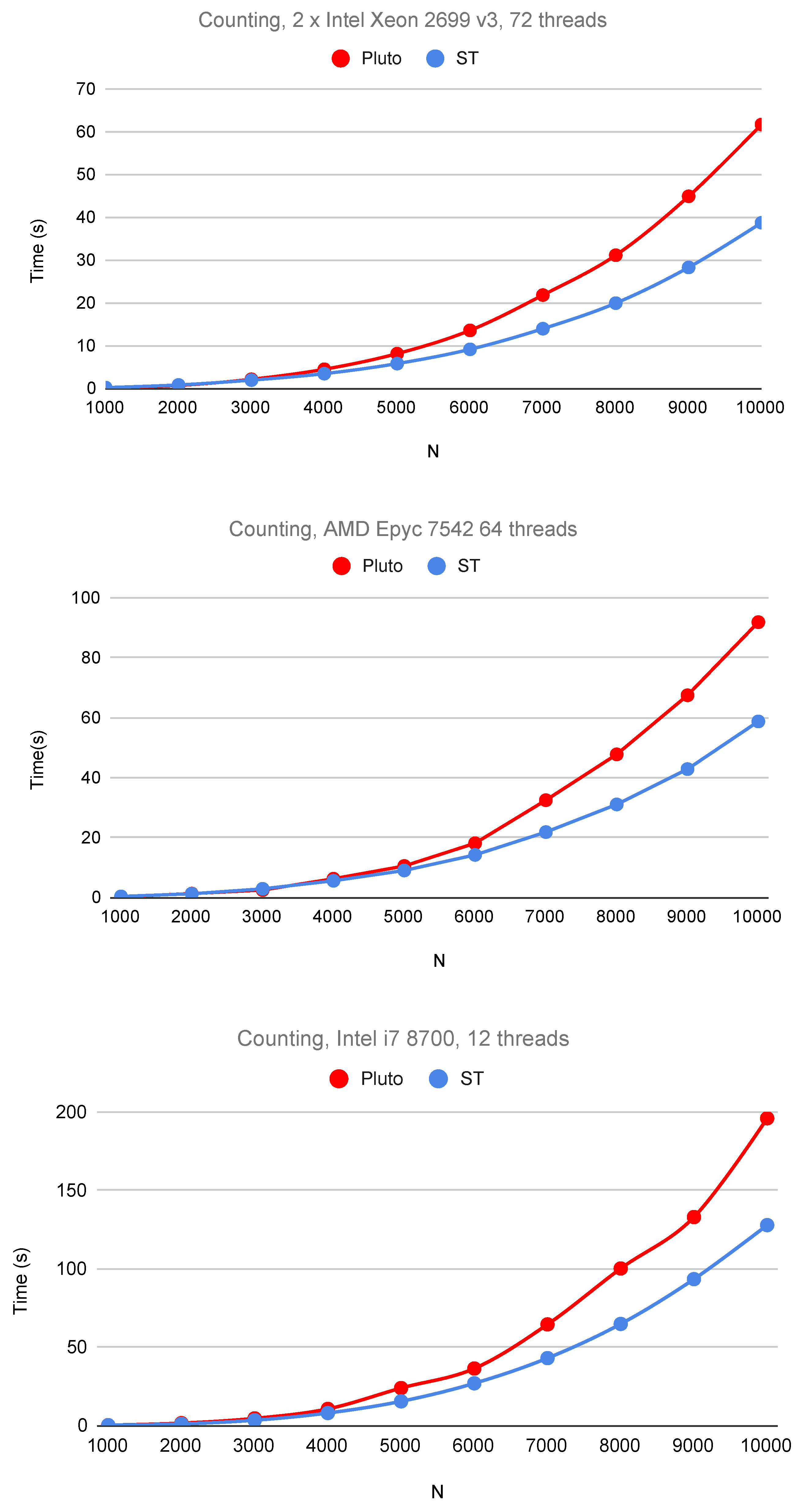
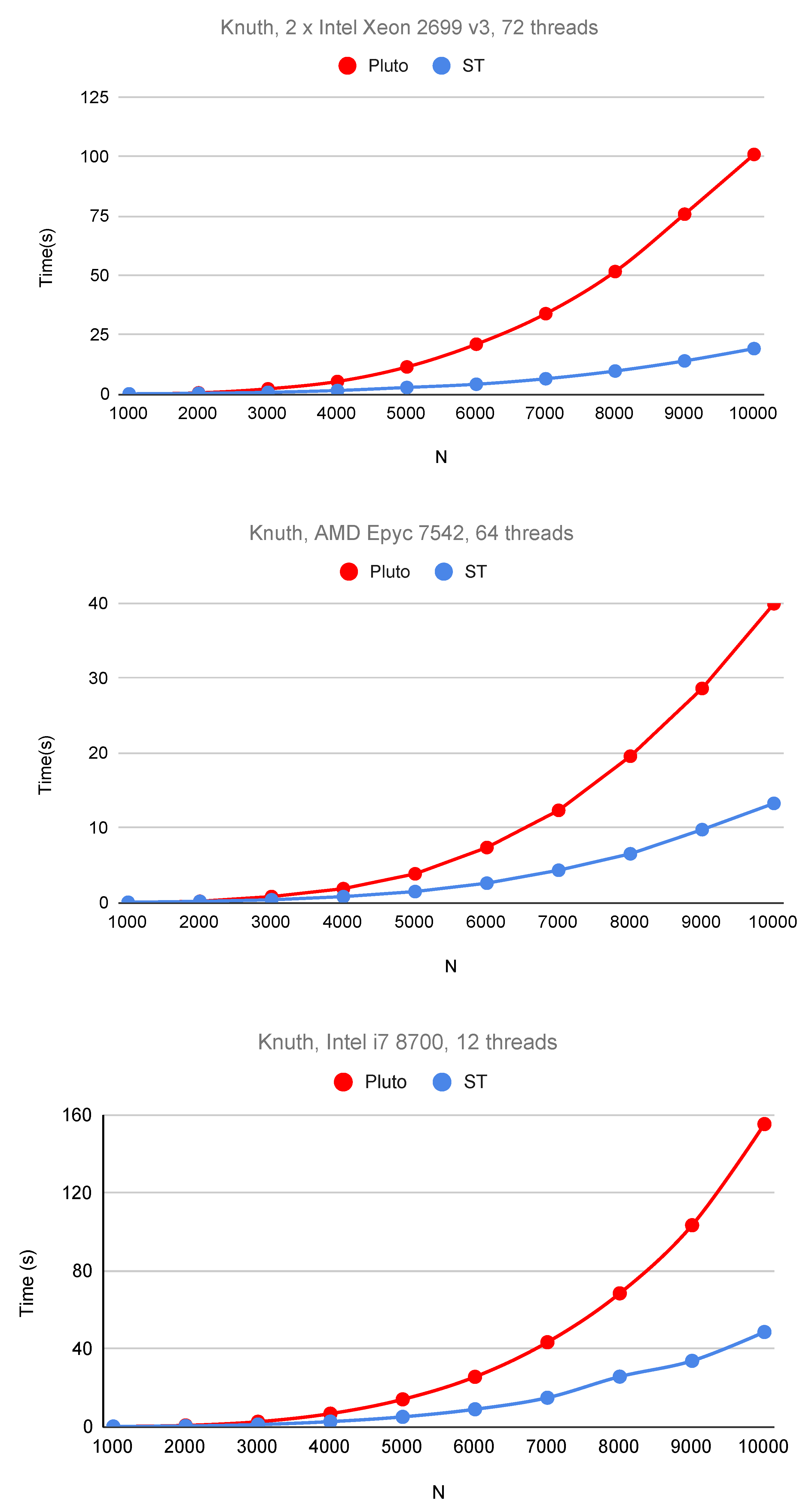
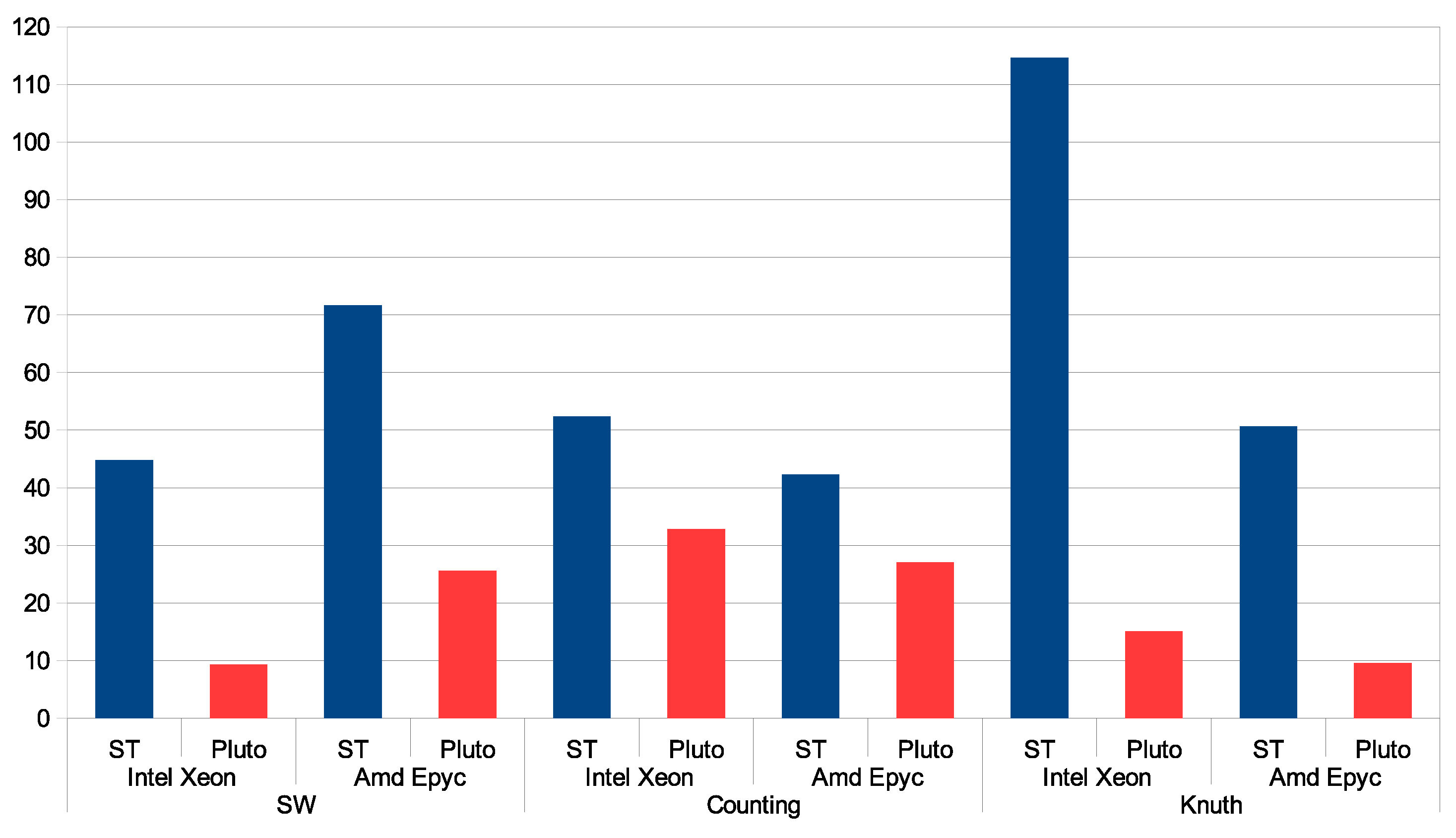
6. Experimental Study

In this section, we present the results of an experimental study with codes implementing the SW, Counting, and Knuth algorithms. Tiled codes were generated by means of PLuTo and TRACO, and they can be found at http://traco.sourceforge.net/dp/sw (accessed on 1 September 2021). All parallel tiled codes were generated by means of the Intel C++ Compiler (icc) and GNU C++ Compiler (g++) with the -O3 flag of optimization.

In order to carry out experiments, we used three multi-processor machines: a 2 × Intel Xeon E5-2699 v3 (2.3 Ghz, 72 threads, 45 MB Cache, and compiler icc 17.0.1), an Intel i7-8700 (3.2 GHz, 4.6 GHz in turbo, 6 cores, 12 threads, 12MB Cache, and compiler icc 19.0.1), and an AMD Epyc 7542 (2.35 GHz, 32 cores, 64 threads, 128MB Cache, and compiler g++ 9.3.0).

For each examined original code, PLuTo generates only 2D tiled code. TRACO implementing space-time tiling (ST) generates 3D tiled code, and the third dimension defines the size of time slices within each 2D space tile.

For each TRACO and PLuTo code generated, we explored many different tile sizes to find the best one resulting in maximal code performance. For TRACO, we empirically found out that tile size $16\times 16\times 16$ allows us to reach maximal performance of all examined codes: the first two dimensions define the size of a space tile, while the third one defines the number of time partitions within a time slice.

Under our experiments, for PLuTo 2D codes, the best tile size among all sizes examined by us is $16\times 16$.

Figure 2 presents the execution times of TRACO and PLuTo parallel tiled codes executed on three machines, 2 × Intel Xeon 2699 v3 (72 threads), Intel i7-8700 (12 threads), and AMD Epyc 7543 (64 threads), for randomly generated sequences of length 1000 to 10,000 and 1000 to 15,000, respectively. As we can observe, the parallel tiled code generated by means of the space-time approach presented in this paper considerably outperforms the one generated with PluTo.

Figure 3 shows the execution times of TRACO and PLuTo parallel tiled codes of the Counting algorithm for randomly generated sequences of length 1000 to 10,000. As we can observe, the parallel space-time tiled code also outperforms the one generated with PLuTo for each studied machine.

Figure 4 presents the execution times of TRACO and PLuTo parallel tiled codes of Knuth’s algorithm for randomly generated sequences of length 1000 to 10,000. Space-time tiling outperforms PLuTo tiling significantly because PLuTo is unable to tile the innermost loop in the Knuth’s code.

Figure 5 depicts speedups of TRACO and PLuTo codes achieved on a 2 × Intel Xeon 2699 v3 (72 threads) and AMD Epyc 7543 (64 threads) for the length of a sequence, $N=$ 10,000. It is worth noting that, for the Intel Xeon, the speedup of the space-time tiled Knuth’s code is greater than 72 (about 114). For the AMD Epyc, the speedup of the SW code is greater than 64. This means that the space-time target parallel codes expose super-linear speedup on the two modern machines.

To summarize, we may conclude that splitting larger unbounded tiles into smaller ones presented with time slices allows us to increase target parallel tiled code locality, which results in increasing its performance for the examined dynamic programming codes.

7. Related Work

In this section, we discuss well-known tiling techniques and compare them with the technique presented in this paper.

Wonnacott et al. introduced serial 3D tiling of “mostly-tileable” loop nests of Nussinov’s RNA secondary structure prediction in [11] to overcome the limitations of affine transformations. However, the authors do not present any method for parallelizing tiled codes.

Mullapudi and Bondhugula [12] have explored automatic techniques for tiling codes that lie outside the domain of affine transformation techniques. Three-dimensional iterative tiling for dynamic scheduling is calculated by means of re-orderable reduction chains to eliminate cycles among tiles in the dependence graph for Nussinov’s algorithm. Their approach involves dynamic scheduling of tiles rather than the generation of a static code.

Li and et al. showed how to use array transposition to enable better caching for Nussinov’s algorithm [2] by replacing the array reading column order to the row order storing transposed cells in the unused lower triangle of Nussinov’s array. However, that approach is restricted to Nussinov’s folding only, and it is not clear how other DP algorithms can be optimized.

Sophisticated tile shapes such as diamond and hexagonal tiling are presented in papers [30,31]. The approaches presented in those papers can deal with loop nests exposing affine dependences. However, those tile shapes cannot be applied to other programs other than stencils. They also do not use time slices within a larger tile to form smaller target tiles. For example, hexagonal tiling constructs a hexagonal tile shape along the time axes of a stencil code and the first space dimension and classical tiling along the other space dimensions. The idea for using time slices in order to form target tiles presented in this paper was not considered in diamond and hexagonal tiling.

Diamond tiling is enabled by the PLuTo compiler. We tried to generate diamond tiling for the loop nests discussed in the previous section by means of PLuTo. For each of those loop nests, PLuTo failed to generate diamond tiling.

Loop tiling based on a tile correction technique [32] generates tiles of irregular shapes and sizes [20]. This complicates thread load balancing during tile code execution, and it simultaneously does not guarantee that, for a larger tile, all data associated with that tile are held in the cache. This results in decreasing code performance.

Paper [33] introduces the Multi-Way Autogen framework, which first combines mono-parametric tiling of the input iterative DP code with loop-to-recursion conversion in order to obtain a parametrically recursive divide-and-conquer algorithm. Then, it decomposes a loop nest into several pieces in order to expose additional parallelism across loop iterations and across recursive calls. Mono-parametric tiling is based on deriving and applying affine transformations to generate target code. So, it fails to tile the innermost loop in the codes examined in our paper, i.e., the target space tiles are unbounded. In order to allow for parallelism and to improve target code locality, the authors suggest decomposing a loop nest into smaller ones and then recursive calls are used so that all inter-tile dependences are respected. Autogen only considers DP algorithms which have a single-assignment statement in them. Since the paper [33] does not contain any full target codes and does not provide any link to Autogen, we are not able to present any comparisons of the performance of codes generated by means of our technique and the ones introduced in paper [33].

8. Conclusions

The paper presents a novel approach for space-time loop tiling implemented in the publicly available TRACO compiler. First, for each loop nest statement, subspaces are generated so that the intersection of them results in tiles, which can be enumerated in lexicographical order or in parallel by means of the wave-front technique. Then, within each tile, time slices are formed, which are enumerated in lexicographical order. The approach was applied to the three dynamic programming applications in order to generate parallel tiled code. The results of carried out experiments with that code demonstrate satisfactory code speedup and scalability. For the same original codes, we applied the state-of-the-art PLuTo compiler, which forms and applies affine transformations in order to generate parallel tiled code. We presented the results of the comparison of code performance.

We experimentally discovered that the proposed approach to generate parallel tiled code has an advantage over affine transformation techniques when they fail to tile the innermost loop in a nest of loops that results in the generation of unbounded tiles. In such a case, code locality is poor. Splitting unbounded space tiles into smaller ones represented with time slices within each space tile allows us to increase code locality and preserve enough target code parallelism to be run on modern multi-core computers.

In the future, we will enlarge space-time tiling with more advanced strategies of sub-space generation that is not limited to only the rectangular shape. We plan to study space-time loop tiling relative to more dynamic programming tasks, exposing affine dependence patterns preventing or making only affine transformations inefficient relative to the tiles and parallelizing such tasks.

References

1. Liu, L.; Wang, M.; Jiang, J.; Li, R.; Yang, G. Efficient Nonserial Polyadic Dynamic Programming on the Cell Processor. In Proceedings of the 2011 IEEE International Symposium on Parallel and Distributed Processing Workshops and Phd Forum, Anchorage, AK, USA, 16–20 May 2011; pp. 460–471. [Google Scholar]
2. Li, J.; Ranka, S.; Sahni, S. Multicore and GPU algorithms for Nussinov RNA folding. BMC Bioinform. 2014, 15, S1. [Google Scholar] [CrossRef] [PubMed] [Green Version]
3. Zhao, C.; Sahni, S. Cache and energy efficient algorithms for Nussinov’s RNA Folding. BMC Bioinform. 2017, 18, 518. [Google Scholar] [CrossRef] [PubMed] [Green Version]
4. Frid, Y.; Gusfield, D. An improved Four-Russians method and sparsified Four-Russians algorithm for RNA folding. Algorithms Mol. Biol. 2016, 11, 22. [Google Scholar] [CrossRef] [PubMed] [Green Version]
5. Jacob, A.; Buhler, J.; Chamberlain, R.D. Accelerating Nussinov RNA Secondary Structure Prediction with Systolic Arrays on FPGAs. In Proceedings of the 2008 International Conference on Application-Specific Systems, Architectures and Processors, Leuven, Belgium, 2–4 July 2008; pp. 191–196. [Google Scholar] [CrossRef] [Green Version]
6. Mathuriya, A.; Bader, D.A.; Heitsch, C.E.; Harvey, S.C. GTfold: A Scalable Multicore Code for RNA Secondary Structure Prediction. In Proceedings of the 2009 ACM Symposium on Applied Computing, New York, NY, USA, 8–12 March 2009; pp. 981–988. [Google Scholar]
7. Markham, N.R.; Zuker, M. UNAFold. In Bioinformatics: Structure, Function and Applications; Keith, J.M., Ed.; Humana Press: Totowa, NJ, USA, 2008; pp. 3–31. [Google Scholar]
8. Lorenz, R.; Bernhart, S.H.; Höner zu Siederdissen, C.; Tafer, H.; Flamm, C.; Stadler, P.F.; Hofacker, I.L. ViennaRNA Package 2.0. Algorithms Mol. Biol. 2011, 6, 26. [Google Scholar] [CrossRef]
9. Trifunovic, K.; Nuzman, D.; Cohen, A.; Zaks, A.; Rosen, I. Polyhedral-model guided loop-nest auto-vectorization. In Proceedings of the 2009 18th International Conference on Parallel Architectures and Compilation Techniques, Raleigh, NC, USA, 12–16 September 2009; pp. 327–337. [Google Scholar]
10. Palkowski, M.; Bielecki, W. Parallel tiled Nussinov RNA folding loop nest generated using both dependence graph transitive closure and loop skewing. BMC Bioinform. 2017, 18, 290. [Google Scholar] [CrossRef] [Green Version]
11. Wonnacott, D.; Jin, T.; Lake, A. Automatic tiling of “mostly-tileable” loop nests. In Proceedings of the IMPACT 2015: 5th International Workshop on Polyhedral Compilation Techniques, Amsterdam, The Netherlands, 19–21 January 2015. [Google Scholar]
12. Mullapudi, R.T.; Bondhugula, U. Tiling for Dynamic Scheduling. In Proceedings of the 4th International Workshop on Polyhedral Compilation Techniques, Vienna, Austria, 20 January 2014; Rajopadhye, S., Verdoolaege, S., Eds.; 2014. Available online: https://acohen.gitlabpages.inria.fr/impact/impact2014/ (accessed on 1 September 2021).
13. Bondhugula, U.; Hartono, A.; Ramanujam, J.; Sadayappan, P. A practical automatic polyhedral parallelizer and locality optimizer. In Proceedings of the 29th ACM SIGPLAN Conference on Programming Language Design and Implementation, London, UK, 15–20 June 2008; Volume 43, pp. 101–113. [Google Scholar]
14. Griebl, M. Automatic Parallelization of Loop Programs for Distributed Memory Architectures; Univ. Passau: Passau, Germany, 2004. [Google Scholar]
15. Irigoin, F.; Triolet, R. Supernode partitioning. In Proceedings of the 15th ACM SIGPLAN-SIGACT Symposium on Principles of Programming Languages, POPL88, San Diego, CA, USA, 10–13 January 1988; ACM: New York, NY, USA, 1988; pp. 319–329. [Google Scholar]
16. Lim, A.; Cheong, G.I.; Lam, M.S. An Affine Partitioning Algorithm to Maximize Parallelism and Minimize Communication. In Proceedings of the 13th international conference on Supercomputing, Rhodes, Greece, 20–25 June 1999; ACM Press: Portland, OR, USA, 1999; pp. 228–237. [Google Scholar]
17. Ramanujam, J.; Sadayappan, P. Tiling multidimensional itertion spaces for multicomputers. J. Parallel Distrib. Comput. 1992, 16, 108–120. [Google Scholar] [CrossRef]
18. Wolf, M.E.; Lam, M.S. A data locality optimizing algorithm. In Proceedings of the Proceedings of the ACM SIGPLAN 1991 Conference on Programming Language Design and Implementation, Toronto, Canada, 24–28, June 1991; Volume 26, pp. 30–44. [Google Scholar]
19. Xue, J. Loop Tiling for Parallelism; Kluwer Academic Publishers: Norwell, MA, USA, 2000. [Google Scholar]
20. Bielecki, W.; Skotnicki, P. Insight into tiles generated by means of a correction technique. J. Supercomput. 2019, 75, 2665–2690. [Google Scholar] [CrossRef] [Green Version]
21. Palkowski, M.; Bielecki, W. Tuning iteration space slicing based tiled multi-core code implementing Nussinov’s RNA folding. BMC Bioinform. 2018, 19, 12. [Google Scholar] [CrossRef] [PubMed] [Green Version]
22. Smith, T.; Waterman, M. Identification of common molecular subsequences. J. Mol. Biol. 1981, 147, 195–197. [Google Scholar] [CrossRef]
23. Waterman, M.S.; Smith, T.F. RNA secondary structure: A complete mathematical analysis. Math. Biosci. 1978, 42, 257–266. [Google Scholar] [CrossRef]
24. Knuth, D.E. Optimum binary search trees. Acta Inform. 1971, 1, 14–25. [Google Scholar] [CrossRef]
25. Bondhugula, U. Effective Automatic Parallelization and Locality Optimization Using the Polyhedral Model. Ph.D. Thesis, The Ohio State University, Columbus, OH, USA, 2008. [Google Scholar]
26. Verdoolaege, S.; Grosser, T. Polyhedral Extraction Tool. In Proceedings of the 2nd International Workshop on Polyhedral Compilation Techniques, Paris, France, 23 January 2012. [Google Scholar]
27. Verdoolaege, S. Counting affine calculator and applications. In Proceedings of the First International Workshop on Polyhedral Compilation Techniques (IMPACT’11), Charmonix, France, 3 April 2011. [Google Scholar]
28. Verdoolaege, S.; Janssens, G. Scheduling for PPCG. Report CW 2017, 706. [Google Scholar] [CrossRef]
29. Wolfe, M. Loops skewing: The wavefront method revisited. Int. J. Parallel Program. 1986, 15, 279–293. [Google Scholar] [CrossRef]
30. Bondhugula, U.; Bandishti, V.; Pananilath, I. Diamond tiling: Tiling techniques to maximize parallelism for stencil computations. IEEE Trans. Parallel Distrib. Syst. 2016, 28, 1285–1298. [Google Scholar] [CrossRef]
31. Grosser, T.; Cohen, A.; Holewinski, J.; Sadayappan, P.; Verdoolaege, S. Hybrid hexagonal/classical tiling for GPUs. In Proceedings of the Annual IEEE/ACM International Symposium on Code Generation and Optimization, Orlando, FL, USA, 14–15 February 2014; pp. 66–75. [Google Scholar]
32. Bielecki, W.; Palkowski, M. Tiling arbitrarily nested loops by means of the transitive closure of dependence graphs. Int. J. Appl. Math. Comput. Sci. (AMCS) 2016, 26, 919–939. [Google Scholar] [CrossRef] [Green Version]
33. Javanmard, M.M.; Ahmad, Z.; Kong, M.; Pouchet, L.N.; Chowdhury, R.; Harrison, R. Deriving parametric multi-way recursive divide-and-conquer dynamic programming algorithms using polyhedral compilers. In Proceedings of the 18th ACM/IEEE International Symposium on Code Generation and Optimization, San Diego, CA, USA, 22–26 February 2020; pp. 317–329. [Google Scholar]
Figure 1. Spaces and tiles. (a) Spaces and time slices; (b) Target tiles.
Electronics 10 02233 g001
Figure 2. Running times of the parallel tiled Smith–Waterman implementations generated by applying space-time tiling and PLuTo.
Electronics 10 02233 g002
Figure 3. Running times of the parallel tiled Counting implementations generated by applying space-time tiling and PLuTo.
Electronics 10 02233 g003
Figure 4. Running times of the parallel tiled Knuth OBST implementations generated by applying space-time tiling and PLuTo.
Electronics 10 02233 g004
Figure 5. Speedup of tiled codes on a 2 × Intel Xeon 2699 v3 (72 threads) and AMD Epyc 7543 (64 threads) for N = 10,000.
Electronics 10 02233 g005