Periodic Event-Triggered Estimation for Networked Control Systems

Abstract

This paper considers the problem of remote state estimation in a linear discrete invariant system, where a smart sensor is utilized to measure the system state and generate a local estimate. The communication depends on an event scheduler in the smart sensor. When the channel between the remote estimator and the smart sensor is activated, the remote estimator simply adopts the estimate transmitted by the smart sensor. Otherwise, it calculates an estimate based on the available information. The closed-form of the minimum mean-square error (MMSE) estimator is introduced, and we use Gaussian preserving event-based sensor scheduling to obtain an ideal compromise between the communication cost and estimation quality. Furthermore, we calculate a variation range of communication probability, which helps to design the policy of event-triggered estimation. Finally, the simulation results are given to illustrate the effectiveness of the proposed event-triggered estimator.

1. Introduction

With the development and high efficiency requirements of communication engineering, control science, industrial automation and computer technology, networked control systems (NCSs) have been gaining more attention and much research interest in recent years. NCSs are widely used within many areas, such as public transportation, military defense, health care, etc. [1]. A NCS often contains a huge communication network, where sensors and actuators are linked together, and components in the communication network transmit their updates to a fusion center. Such a communication network makes a NCS work more efficiently. Due to NCSs’ high efficiency in industrial engineering, they have been widely studied and explored in practice, but there are still many challenges to be solved in the system design of NCSs.

One challenge is the estimation problem of NCSs. Since state estimation is completed in a fusion center by using sensor data transmitted over communication networks, it leads to a high cost. Moreover, a NCS often adopts remote sensors and actuators, making the system transmission more efficient.

Previous results on event-based estimation have two lines. One line focuses on the design of optimal-triggering policies. The optimal event-based sensor transmission scheduling problem of a scalar system was studied in [2] with a finite horizon; the result was extended to a vector system in [3], which significantly reduced the communication cost. For the distributed estimation problem, Weimer and James in [4] proposed a distributed event-triggered estimation algorithm. A model-based adaptive event-triggered control scheme was also presented in [5] for a class of uncertain single-input and single-output nonlinear continuous-time systems. Unlike the above results, adopting a deterministic event-based schedule, in [6], an optimal stochastic event-triggered estimation policy was studied, and the results were extended to a multi-sensors case in [7]. Furthermore, an optimal event-triggered tracking control scheme was also proposed for completely unknown nonlinear systems under the adaptive dynamic programming (ADP) framework in [8]. For more research in this line, see also [9,10,11]. In this field, researchers mainly study for an optimal event-triggered policy, which may not run for an optimal estimation.

In addition to the optimal event policy, another line is to find the optimal estimation for a given event-triggered schedule; many relevant studies have been carried out recently. A stochastic state estimator, which is suitable for event-sampling strategies, was designed in [12] without energy constraints. However, considering the fact that sensors are usually with energy constraints in practical cases, an event-triggered estimation with energy constraints was probed in [13], based on hidden Markov models. When sensors can harvest energy to overcome energy constraints, Huang et al. applied an event-triggered estimator to NCSs in [14]. The problem of real-time reachable set control for a class of singular Markov jump networked cascade systems with time-delay, disturbance and non-zero initial conditions, was considered in [15]. For subsequent results of similar studies, see also [16,17,18]. Although an optimal estimation can be found in this way, an event-triggered approach also needs to be studied for a better transmission effect.

In this work, the policy of an event-triggered system is studied to trade off between the transmission cost and communication quality, and we find the system can improve the estimation effect when the event is not triggered. The main contributions of this paper are summarized as follows:

• A periodic event-triggered transmitting policy is discussed to innovatively handle the specific relationship between the communication cost and effect.
• The transmission effect is also compared under different triggering probabilities. When the transmission rate is improved, the error covariances of the estimates are decreased. A fair comparative study is also presented to demonstrate the necessity of considering a periodic transmitting policy in reality.

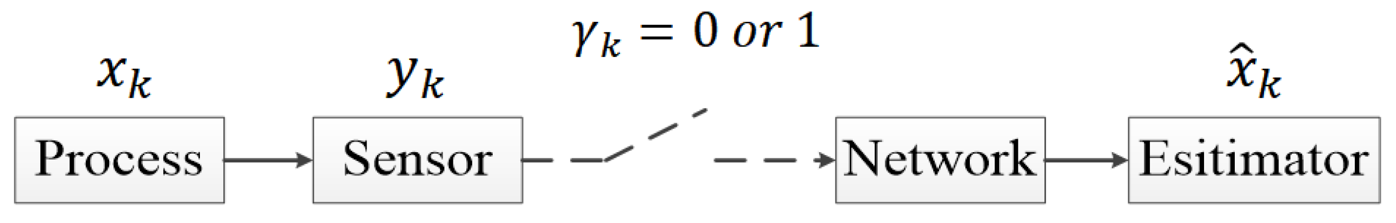
We organized the rest of this paper as follows: the problem formulation and the system modal shown in Figure 1 are presented in Section 2, with the description of the local sensor and remote state estimate. Section 3 presents the expression of the MMSE estimate, and studies the relationship between the transmission cost and efficiency with a periodic event-triggered policy. Section 4 provides some specific simulation results. The concluding remarks are given at the end.

Notations: Let $\mathbb{Z}$ denote the set of all integers, and $\mathbb{N}$ the positive integers. ${\mathbb{S}}_{+}^n$ and ${\mathbb{S}}_{++}^n$ are the sets of $n\times n$ positive semi-definite and positive definite matrices. For example, when $X\in {\mathbb{S}}_{+}^n$, we write $X⩾0$ ($X>0$, if $X\in {\mathbb{S}}_{++}^n$ ). Similarly, if $X-Y\in {\mathbb{S}}_{+}^n$, we obtain $X⩾Y$. $\mathbb{R}$ is the set of real numbers, and ${\mathbb{R}}^n$ the n-dimensional Euclidean space. $Tr(·)$ stands for the trace of a matrix. $Pr(·)$ refers to the probability of a random event. $\mathbb{E}[·]$ represents the expectation of a random event, and $det(·)$ is the determinant of a matrix. ⋀ denotes taking the larger value. For functions $h,h_1,h_2$ with appropriate domains, $h_1\circ h_2\left(x\right)$ is the composite function $h_1\left(h_2\left(x\right)\right)$, and $h^n\left(x\right)\triangleq h\left(h^{n-1}\left(x\right)\right)$, with $h^0\left(x\right)\triangleq x$, where $n\in \mathbb{N}$.

2. Estimation Setup

Consider the linear time-invariant (LTI) system as follows:

$$\begin{array}{cc}\hfill x_{k+1}& =A{x}_k+w_k,\hfill \end{array}$$

(1)

$$\begin{array}{cc}\hfill y_k& =C{x}_k+v_k.\hfill \end{array}$$

(2)

where $k\in \mathbb{N}$. In the system, $x_k\in {\mathbb{R}}^{n_x}$ stands for the state vector at time k, and $y_k\in {\mathbb{R}}^{n_y}$ refers to the measurement received from the sensor. Then, $w_k\in {\mathbb{R}}^{n_x}$ and $v_k\in {\mathbb{R}}^{n_y}$ represent zero-mean independent and identically distributed Gaussian noises, with $\mathbb{E}\left[w_k{w}_j^{\prime }\right]={\delta }_{kj}Q(Q⩾0)$, $\mathbb{E}\left[v_k{\left(v_j\right)}^{\prime }\right]={\delta }_{kj}R(R>0)$, $\mathbb{E}\left[w_k{\left(v_j\right)}^{\prime }\right]=0$, $\forall j$, $k\in \mathbb{N}$, where ${\delta }_{ij}$ is the Dirac delta function, i.e., if $i=j$, ${\delta }_{ij}$ is equal to 1, and 0 otherwise. For pair $(A,C)$ and $\left(A,Q^{1/2}\right)$, the former is assumed to be detectable and the latter is stabilizable.

The initial state $x_0$ of this LTI system with covariance ${\Theta }_0⩾0$, which is uncorrelated with $w_k$ and $v_k$, is a zero-mean Gaussian random vector.

2.1. Sensor Local Estimate

In the network estimation scheme, sensors are usually embedded in the on-board processor to improve the utilization of computing capabilities, which can promote the system performance significantly as explained in [19]. A number of previous studies, such as [20,21], have focused on the “smart sensor” in the system. It runs a Kalman filter locally at each time k and calculates the MMSE estimate of the state $x_k$, according to all the measurement results up to time k. The sensor firstly collects the value of estimate locally, and then sends to the remote estimator.

For further calculation, we denote the MMSE state estimate of local sensor as ${\widehat{x}}_k^s$:

$$\begin{array}{cc}\hfill {\widehat{x}}_k^s& =\mathbb{E}\left[x_k\mid y_1,y_2,\dots ,y_k\right],\hfill \end{array}$$

(3)

Let $e_k^s$ and $P_k^s$ stand for the corresponding estimation error and respective error covariance, which are given by the following:

$$\begin{array}{cc}\hfill e_k^s& =x_k-{\widehat{x}}_k^s,\hfill \end{array}$$

(4)

$$\begin{array}{cc}\hfill P_k^s& =\mathbb{E}\left[\left(x_k-{\widehat{x}}_k^s\right){\left(x_k-{\widehat{x}}_k^s\right)}^{\prime }\mid y_1,y_2,\dots ,y_k\right].\hfill \end{array}$$

(5)

The recursive standard Kalman filter equations in [14] are shown as follows:

$$\begin{array}{cc}{\widehat{x}}_{k\mid k-1}^s& =A{\widehat{x}}_{k-1}^s,\end{array}$$

(6)

$$\begin{array}{cc}{P}_{k\mid k-1}^s& =A{P}_{k-1}^s{A}^{\prime }+Q,\end{array}$$

(7)

$$\begin{array}{cc}\hfill K_k^s& =P_{k\mid k-1}^s{C}^{\prime }{\left[C{P}_{k\mid k-1}^s{C}^{\prime }+R\right]}^{-1},\hfill \end{array}$$

(8)

$$\begin{array}{cc}\hfill {\widehat{x}}_k^s& =A{\widehat{x}}_{k-1}^s+K_k^s\left(y_k-CA{\widehat{x}}_{k-1}^s\right),\hfill \end{array}$$

(9)

$$\begin{array}{cc}\hfill P_k^s& =\left(I-K_k^{s}C\right)P_{k\mid k-1}^s.\hfill \end{array}$$

(10)

where the recursion starts from $P_0^s={\Theta }_0⩾0$ with ${\widehat{x}}_0^s=0$.

As is shown in some previous studies, such as the standard Kalman filter analysis in [16], $P_k^s$ in (10), which denotes the estimation error covariance, converges to a steady state value by an exponential rate.

To facilitate the discussion, the following operators h and $\tilde{g}$ are proposed, which satisfy ${\mathbb{S}}_{+}^n\to {\mathbb{S}}_{+}^n$:

$$\begin{array}{cc}\hfill h\left(X\right)& \triangleq AX{A}^{\prime }+Q,\hfill \end{array}$$

(11)

$$\begin{array}{cc}\hfill \tilde{g}\left(X\right)& \triangleq X-X{C}^{\prime }{\left[CX{C}^{\prime }+R\right]}^{-1}CX,\hfill \end{array}$$

(12)

$$\begin{array}{cc}\hfill h^k\left(X\right)& \triangleq \underset{k\mathrm{times}}{\underbrace{h\circ h\circ \cdots \circ h\circ h}}\left(X\right).\hfill \end{array}$$

(13)

The Kalman filter on the sensor side will enter a steady state value, that is:

$$\begin{array}{c}\hfill P_k^s=\overline{P},k⩾0,\end{array}$$

(14)

where $\overline{P}$ is denoted as the steady-state error covariance, i.e., $\tilde{g}\circ h\left(\overline{P}\right)=\overline{P}$.

2.2. Remote State Estimation

In this work, a novel policy is presented for a control system with a smart sensor case. To describe the state estimation, we consider the Gaussianity-preserving communication scheduling policy $\widehat{\Delta }$, where the sensor randomly generates a uniformly distributed random variable ${\xi }_k\in [0,1]$ at each time k, i.e.,

$$\begin{array}{c}\hfill {\gamma }_k=\left\{\begin{array}{cc}0,\hfill & \mathrm{if}{\xi }_k\le s\left(z_k,\Gamma \right),\hfill \\ 1,\hfill & \mathrm{otherwise}.\hfill \end{array}\right.\end{array}$$

(15)

where $z_k$ stands for the information related with the transmission probability, which is described specifically later. For (15), we define $s(x,\Gamma )$ as

$$s(x,\Gamma )=e^{-\frac{1}{2}{x}^{\prime }{\Gamma }^{-1}x},$$

where $x\in {\mathbb{R}}^n$, and $\Gamma \in {\mathbb{S}}_{+}^n$ is designed to be a weight matrix.

As is shown in (15), if the value of $s\left(z_k,\Gamma \right)$ is smaller, the probability of ${\gamma }_k$ is lower at each time k. Under this situation, the communication between sensor and estimator is more likely to be triggered.

Since the event trigger is stochastical, it is possible that the communication may not be activated for a long time. In order to enhance the robustness of the system, we define ${\lambda }_k\left(T\right)$ as the event-triggered period, i.e.,

$$\begin{array}{c}\hfill {\lambda }_k\left(T\right)=\left\{\begin{array}{cc}1,\hfill & k\mathrm{mod}T=1,\hfill \\ 0,\hfill & \mathrm{otherwise}.\hfill \end{array}\right.\end{array}$$

(16)

then, we have the following:

$$\begin{array}{c}\hfill {\overline{\gamma }}_k={\gamma }_k\bigwedge {\lambda }_k,\end{array}$$

(17)

where, if ${\overline{\gamma }}_k=1$, the communication ${\widehat{x}}_k^s$ is sent; otherwise, ${\widehat{x}}_k^s$ is not sent.

$I_k$ is defined to stand for the set of all the information, which is available to the remote estimator up to time k, that is, the following:

$$\begin{array}{c}\hfill I_k=\left\{{\overline{\gamma }}_1{\widehat{x}}_1^s,{\overline{\gamma }}_2{\widehat{x}}_2^s,\dots ,{\overline{\gamma }}_k{\widehat{x}}_k^s\right\}\cup \left\{{\overline{\gamma }}_1,{\overline{\gamma }}_2,\dots ,{\overline{\gamma }}_k\right\}.\end{array}$$

(18)

To better introduce this policy, we let $z_k$ represent the information sent by the local sensor, which is also the incremental innovative information of ${\widehat{x}}_k^s$:

$$\begin{array}{c}\hfill z_k\triangleq {\widehat{x}}_k^s-A^{{\tau }_{k-1}}{\widehat{x}}_{N_{k-1}}^s,\end{array}$$

(19)

where $N_k\triangleq max\left\{j:{\overline{\gamma }}_j=1,1\le j\le k\right\}$ and ${\tau }_k\triangleq k-N_k+1$. $N_k$ stands for the most recent sending instance before time k, while ${\tau }_k$ denotes the distance between time $k+1$ and $N_k$, both of which are measurable to $I_k$.

In order to obtain the MMSE estimate at the remote estimator, ${\widehat{x}}_k$ is denoted as the remote estimator’s own MMSE state estimate, which is based on $I_k$, and $P_k$ the corresponding error covariance, i.e.,

$$\begin{array}{cc}\hfill {\widehat{x}}_k& =\mathbb{E}\left[x_k\mid I_k\right],\hfill \end{array}$$

(20)

$$\begin{array}{cc}\hfill P_k& =\mathbb{E}\left[\left(x_k-{\widehat{x}}_k\right){\left(x_k-{\widehat{x}}_k\right)}^{\prime }\mid I_k\right].\hfill \end{array}$$

(21)

Once the remote estimator successfully receives the estimate by the local sensor’s side, using the system model (1) and (2), it synchronizes its own estimate with that of the sensor. Otherwise, if the estimate is not transmitted, the estimator just predicts $x_k$ recursively based on its available information.

3. Online Sensor Schedule

In this section, a further discussion about the online sensor schedule is carried out. We show the MMSE estimate of the state at each time k, investigate the upper and lower bounds of no transmission probability, and adopt a periodic communication strategy, which can trade off between the cost and efficiency of the system.

3.1. MMSE Estimation

In the following lemma, $\widehat{\Delta }$ in (15) is used to illustrate a computation method. Without loss of generality, if the communication is absent at time k, the conditional distribution of $x_k$ still keeps its Gaussianity, which is elementary for calculating the MMSE estimate and the corresponding estimation error covariance.

Lemma 1.

Let $p_{\widehat{\Delta }}$ represent a probability density. Whenever the transmission is successful, the conditional distribution of $x_k$ keeps the Gaussianity as given $I_k$, i.e.,

$$\begin{array}{c}\hfill p_{\widehat{\Delta }}\left(x_k,x\mid I_k\right)\sim \left\{\begin{array}{cc}\mathcal{N}\left({\widehat{x}}_k^s,P_k^s\right),\hfill & \mathrm{if}{\overline{\gamma }}_k=1,\hfill \\ \mathcal{N}\left(A^{{\tau }_k-1}{\widehat{x}}_{{\mathrm{N}}_k}^s,P_k^s+{\Psi }_k\right),\hfill & \mathrm{if}{\overline{\gamma }}_k=0,\hfill \end{array}\right.\end{array}$$

where ${\Psi }_k$ is calculated by the recursive equations as follows:

$$\begin{array}{c}\hfill {\Sigma }_k=\left(1-{\overline{\gamma }}_{k-1}\right)A{\Psi }_{k-1}{A}^{\prime }+h\left(P_{k-1}^s\right)-P_k^s\end{array}$$

(22)

$$\begin{array}{c}\hfill {\Psi }_k={\left({\Sigma }_k^{-1}+{\Gamma }^{-1}\right)}^{-1}\end{array}$$

(23)

with initial value ${\Psi }_0=0$.

Proof of Lemma 1.

The proofs are straightforward from Lemma 1. We define ${\tilde{z}}_k={\widehat{x}}_k^s-A{\widehat{x}}_{k-1}^s$. Evidently, from (19), we have $z_k={\sum }_{j=N_{k-1}+1}^k{A}^{k-j}{\tilde{z}}_j$. As a result, the lemma can be readily set up from [22]. □

Furthermore, some properties of the incremental innovative information ${\tilde{z}}_k$ are critical for the proof of Lemma 1, which are also indicated in the following lemmas. ${\Gamma }^{-1}$, like the Fisher information matrix shown in Lemma 1, stands for the side state information.

Lemma 2.

If the transmission is absent, the probability is shown as follows:

$$\begin{array}{c}\hfill Pr\left({\overline{\gamma }}_k=0\mid I_{k-1}\right)=det{\left({\Psi }_k{\Sigma }_k^{-1}\right)}^{1/2}.\end{array}$$

(24)

Lemma 3.

The following statements on ${\tilde{z}}_k$ hold: (a). ${\tilde{z}}_k$ is zero-mean Gaussian with $\mathbb{E}\left[{\tilde{z}}_k{\tilde{z}}_k^{\prime }\right]=h\left(P_{k-1}^s\right)-P_k^s;$ (b). The sequence of ${\tilde{z}}_k$, i.e., ${\tilde{z}}_1,{\tilde{z}}_2,\dots ,{\tilde{z}}_k$ are independent.

Proof of Lemma 2 and Lemma 3.

At first, theoretical proofs are given for the Gaussianity of $p_{\widehat{\Delta }}\left(z_k,z\mid I_{k-1}\right)$. For $k=1$, we have $z_1={\widehat{x}}_1^s-A{\widehat{x}}_0^s$ and ${\tilde{z}}_1\sim \mathcal{N}\left(0,{\Sigma }_1\right)$ by Lemma 3, where ${\Sigma }_1=h\left(P_0^s\right)-P_1^s$. Assume $p_{\widehat{\Delta }}\left(z_k\mid I_{k-1}\right)\sim \mathcal{N}\left(0,{\Sigma }_k\right)$ and define ${{\rm Y}}_k=\left\{{\Sigma }_k^{1/2}x\right.:\left.x\in {\mathbb{R}}^{\mathrm{n}}\right\}$. Regarding to the Lebesgue measure on ${{\rm Y}}_k$, we obtain the following:

$$\begin{array}{c}\hfill p_{\widehat{\Delta }}\left(z_k,z\mid I_{k-1}\right)=\frac{1}{{\left(2\pi \right)}^{n_x/2}{\left(det{\Sigma }_k\right)}^{1/2}}exp\left(-\frac{1}{2}{z}^{\prime }{\Sigma }_k^{-1}z\right).\end{array}$$

The probability $Pr\left({\overline{\gamma }}_k=0\mid I_{k-1}\right)$ can be computed as follows:

$$\begin{array}{cc}\hfill & Pr\left({\overline{\gamma }}_k=0\mid I_{k-1}\right)\hfill \\ \hfill =& {\int }_{{{\rm Y}}_k}exp\left(-\frac{1}{2}{z}^{\prime }{\Gamma }^{-1}z\right)p_{\widehat{\Delta }}\left(z_k,z\mid I_{k-1}\right)\mathrm{d}z\hfill \\ \hfill =& {\int }_{{{\rm Y}}_k}exp\left(-\frac{1}{2}{z}^{\prime }\left({\Psi }_k^{-1}-{\Sigma }_k^{-1}\right)z\right)p_{\widehat{\Delta }}\left(z_k,z\mid I_{k-1}\right)\mathrm{d}z\hfill \\ \hfill =& {\int }_{{{\rm Y}}_k}\frac{1}{{\left(2\pi \right)}^{n_x/2}{\left(det{\Sigma }_k\right)}^{1/2}}exp\left(-\frac{1}{2}{z}^{\prime }{\Psi }_k^{-1}z\right)\mathrm{d}z\hfill \\ \hfill =& det{\left({\Psi }_k{\Sigma }_k^{-1}\right)}^{1/2},\hfill \end{array}$$

(25)

which completes the proof of Lemma 2.

On the one hand, if ${\overline{\gamma }}_k=0$, the equation of probability density is shown as follows:

$$\begin{array}{cc}\hfill p_{\widehat{\Delta }}\left(z_k,z\mid I_{k-1},{\overline{\gamma }}_k=0\right)=& \frac{Pr\left({\overline{\gamma }}_k=0\mid z_k=z\right)p_{\widehat{\Delta }}\left(z_k,z\mid I_{k-1}\right)}{Pr\left({\overline{\gamma }}_k=0\mid I_{k-1}\right)}\hfill \\ \hfill =& \frac{1}{{\left(2\pi \right)}^{n_x/2}{\left(det{\Psi }_k\right)}^{1/2}}exp\left(-\frac{1}{2}{z}^{\prime }{\Psi }_k^{-1}z\right),\hfill \end{array}$$

(26)

that is, $p_{\widehat{\Delta }}\left(z_k,z\mid I_{k-1},{\overline{\gamma }}_k=0\right)\sim \mathcal{N}\left(0,{\Psi }_k\right).$ Because of $z_{k+1}=A{z}_k+{\tilde{z}}_{k+1}$ shown in Lemma 3, we obtain the following:

$$\begin{array}{c}\hfill p_{\widehat{\Delta }}\left(z_{k+1},z\mid I_{k-1},{\overline{\gamma }}_k=0\right)\sim \mathcal{N}\left(0,{\Sigma }_{k+1}\right),\end{array}$$

where ${\Sigma }_{k+1}=A{\Psi }_k{A}^{\prime }+h\left(P_k^s\right)-P_{k+1}^s$.

On the other hand, if ${\overline{\gamma }}_k=1$, ${\widehat{x}}_k^s$ is transmitted to the estimator successfully. Conditioned on $I_k$, $z_k$ can be calculated by $z_{k+1}={\widehat{x}}_{k+1}^s-A{\widehat{x}}_k^s={\tilde{z}}_{k+1}$. For ${\Sigma }_{k+1}=h\left(P_k^s\right)-P_{k+1}^s$, we have $p_{\widehat{\Delta }}\left(z_{k+1},z\mid I_{k-1},{\overline{\gamma }}_k=1\right)\sim \mathcal{N}\left(0,{\Sigma }_{k+1}\right)$.

From the optimal filtering theory, $x_k-{\widehat{x}}_k^s$ is orthogonal to $z_k$. Since $x_k-{\widehat{x}}_k^s$ and $z_k$ are jointly Gaussian and $x_k-{\widehat{x}}_k^s\sim \mathcal{N}\left(0,P_k^s\right)$, which reaches the conclusion. □

Then, two theorems are put forward in the following discussions to explain that remote estimators compute their own estimate and the covariance of the corresponding estimation error recursively, under schedule $\widehat{\Delta }$. An efficient but simple recursion comes from the Gaussianity of the a posteriori distribution.

Before introducing two theorems, we recall that ${\widehat{x}}_k^s$ and $P_k^s$ are updated at the sensor side locally, by using a standard Kalman filter. We define the MMSE estimator as $E^{*}$.

Theorem 1.

Consider $\widehat{\Delta }$ given in (15). The value of ${\widehat{x}}_k$ in two different cases is studied, i.e.,

$$\begin{array}{c}\hfill {\widehat{x}}_k=\left\{\begin{array}{cc}{\widehat{x}}_k^s,\hfill & \mathrm{if}{\overline{\gamma }}_k=1,\hfill \\ A{\widehat{x}}_{k-1},\hfill & \mathrm{if}{\overline{\gamma }}_k=0,\hfill \end{array}\right.\end{array}$$

(27)

with ${\widehat{x}}_0=0$. Under this schedule, a positive semi-definite matrix for a concise notation can be denoted as follows:

$$\begin{array}{c}\hfill {\Phi }_k\triangleq \left(1-{\overline{\gamma }}_k\right){\Psi }_k\end{array}$$

(28)

Then, ${\Phi }_k$ is computed according to (22), (23) and (28).

Proof of Theorem 1.

Theorem 1 can be directly obtained from Lemma 1 and Lemma 3. □

Theorem 2.

According to the MMSE estimator $E^{*}$ considered in Theorem 1 and $\widehat{\Delta }$ given in (15). We can calculate the estimator’s estimation error covariance $P_k$ as follows:

$$\begin{array}{c}\hfill P_k=P_k^s+{\Phi }_k.\end{array}$$

(29)

Proof of Theorem 2.

The proof of Theorem 2 is readily from Lemma 1 and Lemma 3 and, thus, is omitted. □

The above two theorems describe that, if ${\overline{\gamma }}_k=1$, $\left({\widehat{x}}_k,P_k\right)$ is updated as $\left({\widehat{x}}_k^s,P_k^s\right)$; when ${\overline{\gamma }}_k=0$, ${\Psi }_k$ stands for the remote estimator’s lost performance since the communication is absent. In fact, $P_k^s$ denotes the estimation error of the sensor’s local Kalman filter, as is shown in Theorem 2, and $P_k$ is simply a sum of $P_k^s$. Compared with open-loop predictions, ${\Gamma }^{-1}$ in ${\Psi }_k$ can be interpreted as supplementary information, obtained from the absence of transmission. By using this method, if the local sensor satisfies the capability of running a Kalman filter, the remote estimator updates its estimate at each time k, and gains the associated estimation error covariance in a simple and efficient way.

3.2. The Bounds of the Probability of No Transmission

In order to study the property of communication schedules, we further explore the transmission probability. Since it is difficult to find the exact value of the probability $Pr\left({\overline{\gamma }}_k=0\mid I_{k-1}\right)$, we try to obtain its upper and lower bounds.

Theorem 3.

The upper bound and lower bound of $Pr\left({\overline{\gamma }}_k=0\mid I_{k-1}\right)$ can be calculated as follows:

$$\begin{array}{cc}\hfill {\left(1+trace\left({\Sigma }_k{\Gamma }^{-1}\right)\right)}^{1/2}& \le det{\left({\Psi }_k{\Sigma }_k^{-1}\right)}^{1/2}\le exp\left(\frac{1}{2}trace\left({\Psi }_k{\Sigma }_k^{-1}\right)\right).\hfill \end{array}$$

(30)

Before proving the Theorem 3, Lemma 4 and Lemma 5 are given as follows.

Lemma 4.

When $P\in {\mathbb{S}}_{++}^n$, $\exists M\in {\mathbb{S}}_{++}^n$, s.t. $M^2=P$, $M=M^{\mathrm{T}}.$

Lemma 5.

Assume $detP={\prod }_{i=1}^n{\alpha }_i$, $P\in {\mathbb{S}}_{++}^n$, where ${\alpha }_i$ is the eigenvalue of P, we have the following:

$$\begin{array}{c}\hfill det\left(I+P\right)=\prod _{i=1}^n\left({\alpha }_i+1\right)=1+\sum _{i=1}^n{\alpha }_i+\cdots ⩾1+traceP.\end{array}$$

Proof of Theorem 3.

Consider ${\Psi }_k$ given in (23). We have the following:

$$\begin{array}{c}\hfill {\left({\Psi }_k{\Sigma }_k^{-1}\right)}^{-1}={\left({\left({\Sigma }_k^{-1}+{\Gamma }^{-1}\right)}^{-1}{\Sigma }_k^{-1}\right)}^{-1}={\Sigma }_k\left({\Sigma }_k^{-1}+{\Gamma }^{-1}\right)=I+{\Sigma }_k{\Gamma }^{-1}\end{array}$$

(31)

For the first inequality given in (30), ${\Sigma }_k\in {\mathbb{S}}_{++}^n$, assuming ${\Sigma }_k=M^2$, we have the following:

$$\begin{array}{c}\hfill det\left({\Psi }_k{\Sigma }_k^{-1}\right)=det\left(I+M{\Gamma }^{-1}{M}^{\mathrm{T}}\right)⩾1+trace\left(M{\Gamma }^{-1}{M}^{\mathrm{T}}\right)=1+trace\left({\Sigma }_k{\Gamma }^{-1}\right).\end{array}$$

Then, because of ${\beta }_i+1\le exp\left({\beta }_i\right)$, it is not hard to obtain the following:

$$\begin{array}{c}\hfill det\left(I+P\right)=\prod _{i=1}^n\left({\beta }_i+1\right)⩾exp\left(\sum _{i=1}^n{\beta }_i\right)=exp\left(traceP\right).\end{array}$$

which completes the proof. □

3.3. Periodic Sending Strategy

Since the probability of communication is not an exact value, we try to explore a schedule to better compromise the system cost and efficiency by constraining the probability $\varpi \left({\overline{\gamma }}_k=0\mid I_{k-1}\right)$ and study the transmission process.

Consider the MMSE estimator $E^{*}$, which is given in Theorem 1, and the corresponding estimation error covariance $P_k$ given in Theorem 2. We introduce another operator g: ${\mathbb{S}}_{+}^n\to {\mathbb{S}}_{+}^n$ to facilitate the discussion:

$$\begin{array}{c}\hfill g\left(X\right)\triangleq A{(X^{-1}+{\Gamma }^{-1})}^{-1}{A}^T+h\left(\overline{P}\right)-\overline{P}.\end{array}$$

(32)

Denote the set of ${\Sigma }_k$ during a period as $\Lambda =\left\{{\Sigma }_k\right\}=\left\{\overline{\Sigma },g\left(\overline{\Sigma }\right),\dots ,g^{T-1}\left(\overline{\Sigma }\right)\right\}$, in order to describe the transmission situation at different moments.

Remark 1.

At time k, when ${\overline{\gamma }}_k=0$ in (18), an iterative calculation is required. For example, if ${\overline{\gamma }}_k=0$, ${\Sigma }_k$ is denoted as ${\Sigma }_k=g\left({\overline{\Sigma }}_{k-1}\right)$, and ${\Sigma }_k={\Sigma }_0$ if ${\overline{\gamma }}_k=1$, with ${\Sigma }_0=\overline{\Sigma }$. The worst case is that the information is only sent once as ${\overline{\gamma }}_{{\lambda }_k\left(T\right)=1}={\overline{\gamma }}_{(k\mathrm{mod}T=1)}=1$, in one period, with ${\Sigma }_{T-1}=g^{T-1}\left(\overline{\Sigma }\right)=g^{T-1}\left({\Sigma }_0\right)$.

It is not difficult to see that when $\Gamma$ is determined, the probability of transmission is related to the variance of ${\tilde{z}}_k$, which is defined as ${\beta }_k$. Assuming $P_k$ is set, we introduce an operator $\eta :{\mathbb{S}}_{+}^n\to {\mathbb{S}}_{+}^n$, then we have the following:

$$\begin{array}{c}\hfill {\beta }_k=Pr({\overline{\gamma }}_k=0\mid g\left(\overline{\Sigma }\right))={\eta }_k\left({\Sigma }_k,\Gamma \right)={\eta }_{\Gamma }\left({\Sigma }_k\right),{\Sigma }_k\in \Lambda .\end{array}$$

(33)

Theorem 4.

Let ${\beta }_0=\overline{\eta }(\tilde{\Sigma })$, ${\beta }_i=\overline{\eta }[g^i(\tilde{\Sigma })],i=1,2,\dots ,T-1$. According to (33), a Markov matrix, as follows, can describe the transmission probability:

$$\Theta ={\left[\begin{array}{ccccc}1-{\beta }_0& {\beta }_0& 0& \dots & 0\\ 1-{\beta }_1& 0& {\beta }_1& \ddots & ⋮\\ ⋮& ⋮& \ddots & \ddots & 0\\ 1-{\beta }_{T-2}& 0& \dots & 0& {\beta }_{T-2}\\ 1& 0& 0& 0& 0\end{array}\right]}_{T\times T},$$

$\overline{\varpi }={(I-\Theta )}^{-1}(I-{\Theta }^T)$, where $\overline{\varpi }$ is the transmission probability during a period T.

Proof of Theorem 4.

When $\Gamma$ is fixed, the transmission probability $\overline{\varpi }$ in a period can be calculated as follows:

$$\begin{array}{cc}\hfill \overline{\varpi }=& I+{\Theta }^1+{\Theta }^2+\cdots +{\Theta }^{T-1}.\hfill \end{array}$$

(34)

For $\overline{\varpi }$ in (34), multiply $(I-\Theta )$, we obtain the following:

$$\begin{array}{c}\hfill (I-\Theta )(I+{\Theta }^1+{\Theta }^2+\cdots +{\Theta }^{T-1})=I+{\Theta }^1+\cdots +{\Theta }^{T-1}-{\Theta }^1-\cdots -{\Theta }^T=I-{\Theta }^T.\end{array}$$

It can be concluded that $\overline{\varpi }$ is ${(I-\Theta )}^{-1}(I-{\Theta }^T)$. □

We further compare the transmission probabilities with different $\Gamma$.

Lemma 6.

Given ${\Gamma }_1\le {\Gamma }_2$ in (15), it follows that we have the following:

$$\begin{array}{c}\hfill \overline{\varpi }\left({\Gamma }_1\right)⩾\overline{\varpi }\left({\Gamma }_2\right).\end{array}$$

(35)

where $\overline{\varpi }\left({\Gamma }_k\right)$ stands for the transmission probability during a period T with ${\Gamma }_k$.

Proof of Lemma 6.

If $A>B>0$, let $A=D^2$, then $D^{-1}B{D}^{-T}>0$, we have the following:

$$\begin{array}{cc}\hfill A-B=D^2-& B=D(I-D^{-1}B{D}^{-1})D^T>0,\hfill \\ & I-D^{-1}B{D}^{-T}>0.\hfill \end{array}$$

Because of $1>det(I-D^{-1}B{D}^{-1})>0$, we have the following:

$$\frac{detB}{detA}=\frac{detB}{detD{D}^T}=det{D}^{-1}B{D}^{-T}<1,$$

so $detA>detB.$

Similarly, for ${\Gamma }^{-1}>0$, ${\Gamma }^{-1}=S^{-2}$, $\exists P>Q>0$, s.t. $det(I+P{S}^2)=det(I+SP{S}^{\mathrm{T}})>det(I+SQ{S}^{\mathrm{T}})$, that is $det(I+P{\Gamma }^{-1})>det(I+Q{\Gamma }^{-1})$. For ${\Psi }_k$ in (33), it is trivial that ${\eta }_{\Gamma }\left(P\right)<{\eta }_{\Gamma }\left(Q\right)$ and $g^{k_1}\left(\overline{\Sigma }\right)⩾g^{k_2}\left(\overline{\Sigma }\right)$ with $k_1⩾k_2$. The Lemma can be concluded. □

Lemma 6 shows that the transmission probability varies with different $\Gamma$s within one period. Specifically, it becomes smaller when $\Gamma$ increases, reducing the communication cost and improving the transmission quality of the system at the same time, which deserves to be used in the design of event-triggered systems.

4. Simulation Examples

It is important to have accurate and efficient communication models of the data transmission networks for the design of event-triggered wireless control systems. Yi et al. proposed an event-triggered consensus protocol and a triggering law in [23], which do not require any a priori knowledge of global network parameters. The Markov decision process and Markov game frameworks were also studied to investigate the optimal transmission strategies for the sensors in [24], developing several structural results on the optimal solutions.

In order to illustrate the estimation quality with bounded states, a stable system is simulated as follows:

$$A=\left[\begin{array}{ccc}0.5& 0.3& 0.4\\ 0.1& 0.7& 0.1\\ 0.3& -0.5& 0.6\end{array}\right],C=\left[\begin{array}{ccc}0.5& 1& 2\\ 1& 3& 0.4\\ 1.5& 0.4& 2.5\end{array}\right],$$

$$Q=\left[\begin{array}{ccc}0.4& 0.2& 0.1\\ 0.2& 0.5& 0.3\\ 0.1& 0.3& 0.5\end{array}\right],R=\left[\begin{array}{ccc}0.1& 0.03& 0.05\\ 0.03& 0.1& 0.02\\ 0.05& 0.02& 0.1\end{array}\right].$$

The error covariances of real states, remote and local estimates are calculated with a finite time-horizon T. We first set ${\Sigma }_{\overline{1}}^{-1}=\left[\begin{array}{ccc}5& 0& 0\\ 0& 5& 0\\ 0& 0& 5\end{array}\right]$ and ${\Sigma }_{\overline{2}}^{-1}=\left[\begin{array}{ccc}2& 0& 0\\ 0& 2& 0\\ 0& 0& 2\end{array}\right]$, observing the implementing results and communication times.

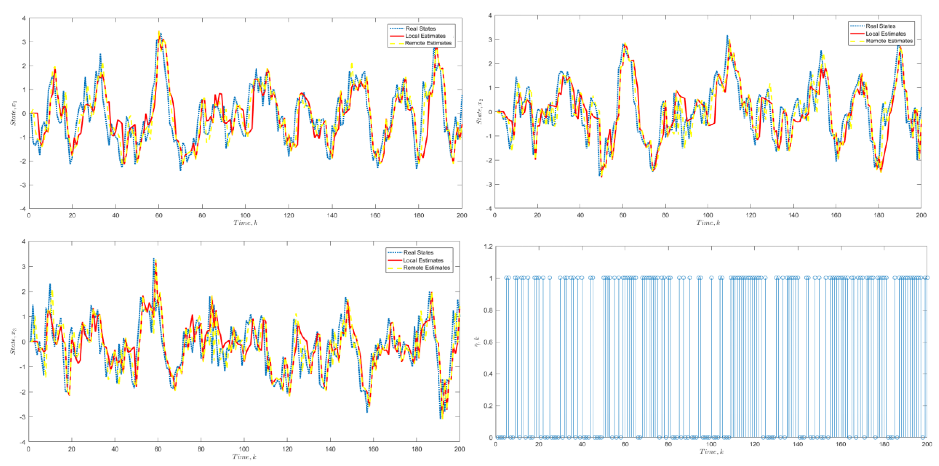
Under ${\Sigma }_{\overline{1}}^{-1}$, the local estimates, remote estimates and real states are approximately the same, as the transmission rate is about 0.45, shown in Figure 2.

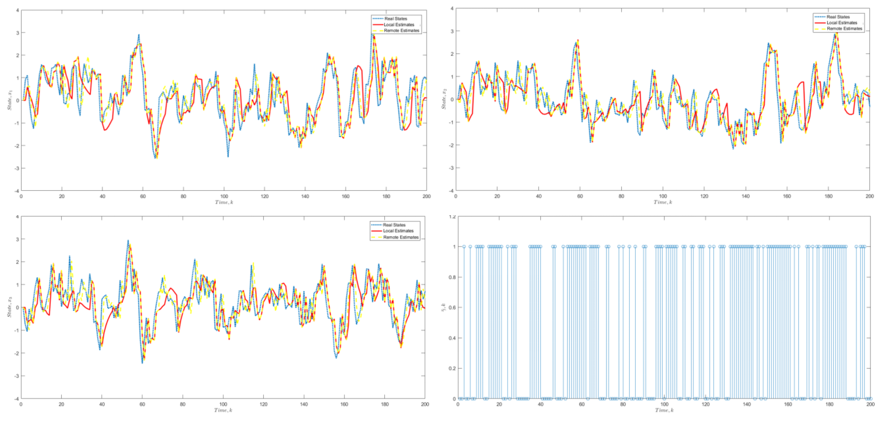
Under ${\Sigma }_{\overline{2}}^{-1}$, the transmission rate is improved to about 0.55, shown in Figure 3, changing between 0.4 and 0.6 generally.

Looking at the figures above, it can be concluded that although the probability of transmission is changed by $\Sigma$, there are few impacts on the state estimation. The local estimates, remote estimates and real states are still roughly the same, as the three different lines in each figure are basically coincident.

We then carry out a fair comparative study with an existing method, considering a case without the periodic transmission schedule. By changing a suitable $\Sigma$, we try to set the transmission rate to about 0.59, shown in Figure 4.

The error covariances of the basic simulations and the comparative study are calculated and shown in

Table 1. The values of error covariances in the above situations.

Time, k	${\mathit{x}}_1$	${\mathit{x}}_2$	${\mathit{x}}_3$
Error Covariance 1$\left({\Sigma }_{\overline{1}}^{-1}\right)$	0.9710	0.8287	0.9210
Error Covariance 2$\left({\Sigma }_{\overline{2}}^{-1}\right)$	0.7268	0.6579	0.8620
Error Covariance 3 (Without the periodic transmission schedule)	0.7795	0.6516	0.6902

, with the above results.

To better test the differences between the two cases, we compare the error covariances in different situations. According to the basic simulations, the error covariances will decrease with a slightly higher transmission rate if the $\Sigma$ increases. The error covariances for the comparative study without the periodic transmission schedule are better than our basic simulations, theoretically, while the event-triggered policy with the periodic communication schedule can guarantee the transmission rate in the system to avoid extreme situations in reality. The innovative periodic transmission schedule in this study helps the system develop the communication quality to a certain extent.

5. Conclusions

In this paper, a remote state estimation problem in a LTI system was studied, where a smart sensor was utilized to measure the system state and generate a local estimate. The Gaussian preserving event-based sensor scheduling and the corresponding closed-form of MMSE estimator were investigated. The variation range of transmission probablity was calculated, which helps to better design the policy of event-triggered estimation. Finally, the effectiveness of proposed estimator was shown through the simulation results.