Explainable Sentiment Analysis: A Hierarchical Transformer-Based Extractive Summarization Approach ^†

Abstract

In recent years, the explainable artificial intelligence (XAI) paradigm is gaining wide research interest. The natural language processing (NLP) community is also approaching the shift of paradigm: building a suite of models that provide an explanation of the decision on some main task, without affecting the performances. It is not an easy job for sure, especially when very poorly interpretable models are involved, like the almost ubiquitous (at least in the NLP literature of the last years) transformers. Here, we propose two different transformer-based methodologies exploiting the inner hierarchy of the documents to perform a sentiment analysis task while extracting the most important (with regards to the model decision) sentences to build a summary as the explanation of the output. For the first architecture, we placed two transformers in cascade and leveraged the attention weights of the second one to build the summary. For the other architecture, we employed a single transformer to classify the single sentences in the document and then combine the probability scores of each to perform the classification and then build the summary. We compared the two methodologies by using the IMDB dataset, both in terms of classification and explainability performances. To assess the explainability part, we propose two kinds of metrics, based on benchmarking the models’ summaries with human annotations. We recruited four independent operators to annotate few documents retrieved from the original dataset. Furthermore, we conducted an ablation study to highlight how implementing some strategies leads to important improvements on the explainability performance of the cascade transformers model.

1. Introduction

As more and more content is shared by people on the web, the use of automated sentiment analysis (SA) tools has become increasingly present. Just think of solutions for monitoring public opinion on social media, or for drawing feedbacks from products or services reviews, to understand what consumers like and do not. Performing SA on free text has already been shown its importance in literature, even in multimodal tasks, where adding features extracted from free text is essential for good performance in sentiment classification of audio and videos [1]. However, today’s systems often lack transparency, as they cannot provide an interpretation of their reasoning. In recent years, this has been a well-known problem in the scientific community. In fact, the contribution that artificial intelligence (AI) algorithms are making in shaping tomorrow’s society is constantly growing. Given the high performance that today’s models can achieve, their application is spanning an increasingly large landscape of fields. This is motivating a rapid paradigm shift in the use of these technologies. We are moving from a paradigm in which AI models are required to deliver the highest possible performance, to one in which such systems are required to provide information about taken decisions that is interpretable by humans. We are referring to the explainable artificial intelligence (XAI) paradigm. As stated by DARPA’s XAI program launched in 2017, the main goal of XAI is to create a suite of models that provide an explanation without affecting performance [2,3,4]. That is, to pass from the concept of black-box models, in which it is hard (or even impossible) to get any sort of explanation from them, to white-box ones, in which the model also provides results that are understandable by the final users, or at least by the experts in the application domain [5]. This may lead systems of the near future to address the needs of government organizations and the users who use them, such as the right to explanation, which can raise the reliability of users in the system, and the right to decision rejection, especially in applications where a human-the-loop approach is expected (Articles 13–15, 22 of the EU GDPR). Additionally, the natural language processing (NLP) community is beginning to approach to this new paradigm [6]. However, the task of explaining NLP systems is certainly not an easy one, in a context where models based on deep neural networks, usually referred to as the least explicable models of machine learning, take the lead. In fact, since the transformer architecture was introduced by Vaswani et al. [7] (Section 2.3), the NLP research has made great strides. In an effort to investigate the behavior of these models and provide some sort of human-understandable interpretation, the weights of the attention mechanism inherent in these structures have often been taken into account (Section 2.5). In this work, we propose and compare two transformer-based models to perform tasks of sentiment analysis, while retrieving an explanation of the models’ decisions through a summary built by extracting the sentences of the document that are the most informative for the task in hand. That is, we exploited the extractive (single document) summarization paradigm (Section 2.2). In particular, for one of the two models, we made use of the attention weights of the transformer model to get insights on the most relevant sentences. To do so, we exploited a hierarchical configuration (Section 2.4). We evaluated our models on a binary sentiment classification task. However, the underlying structures may be easily adapted for any document classification task. To evaluate the classification performance, we used the IMDB movie reviews dataset [8]. To also assess the explainability performance, we annotated some samples of the dataset to retrieve human extractive summaries from the training and test sets, and then assessed the overlap between these and the models’ ones. The annotation phase was necessary since, to the best of our knowledge, this is the first kind of work trying to exploit model architectures to retrieve an extractive summary of a document while performing its sentiment classification (Section 2.1).

The main contributions of this work may be resumed as:

• A new approach to explain document classification tasks as sentiment analysis, by providing extractive summaries as the explanation of the model decision;
• Exploring use of attention weights of a hierarchical transformer architecture as a base to achieve extractive summaries as an explanation of the document classification task;
• A new annotated dataset for the evaluation of extractive summaries as an explanation of a sentiment analysis task. We shared the annotated dataset together with the algorithm code on our Github page (www.github.com/lbacco/ExS4ExSA, accessed on 28 June 2021);
• Two different proposed models, both based on transformer architectures, analyzed in terms of the performance in both the classification and explanation tasks.

Furthermore, we proposed an ablation study for the hierarchical model, to evaluate the impact of (sentence) masking and positional embedding, and the role of the first transformer when it is frozen during the training phase. Additionally, we implemented a new a posteriori metric to evaluate the models’ summaries with no regard to prior annotations.

2. Related Works

2.1. Explainability in Sentiment Analysis

Sentiment analysis, also called opinion mining [9], consists of the classification task of the polarity of some text. In recent years, it has gained interest not only in research but also in industry. It is particularly true due to the advent of blogs and social media, and, thus, the impressive growth that shared content has shown. Organizations are currently using these kind of data for their decision making processes instead of conduct surveys, for example, to rank products or services from the users’ reviews [10] and provide recommendations to the users [11], to predict changes in the stock prices [12], or, to give an example closer to the domain of our work, to predict incomes from movies at the box-office basing the prediction on the online movies’ reviews [13]. In particular, sentiment analysis tasks may be performed at the word, sentence, and document levels. The latter is, of course, the more difficult one to perform because of the greater length of the text, which also may lead to the presence of noisy words or sentences. Longer documents more easily show words and sentences with a polarity that can be neutral or even opposite in respect to the overall polarity of the entire document. This kind of task presents limitations on the interpretability of the decision made by the models. However, in literature, there are not so many works dealing with this side of sentiment analysis models. One way the past literature dealt with the explainable sentiment analysis field was by exploiting a fourth degree of the task, the so-called entity/aspect-based level. Originally called feature-based level [14], it consists of performing a finer-grained analysis by directly looking at the opinions themselves reported in the document. This concept is based on the assumption that each opinion may be seen as the combination of sentiment and its target (the entities and their attributes, the aspects). For example, for the sentence “The photography is nice, but the movie is way too slow” we could say it is a negative comment, but not in its entirety. In fact, we can individuate two entities or aspects (aspect extraction), the photography and the movie, and we can also determine their sentiment (aspect sentiment classification), respectively, as positive and negative. The emphasis on the latter may indicate that the overall score of the sentence is more negative than positive. Thus, combining the aspects’ polarity score, with this approach it is also possible to retrieve an overall polarity score [15], and consequently the document sentiment. This is done while also giving finer-grained insights, for example turning the free text into a structured list of entities and aspects and their associated sentiments. The main disadvantage of this approach is the effort to extract and annotate entities, attributes, and sentiment words or phrases, while also dealing with the presence of implicit aspects. Another way to explore the explainability in sentiment analysis exploited by the past literature is to use the so-called sentiment lexicons. Such items are de facto dictionaries in which words (but also phrases) are associated with some polarity score. The main advantage of this kind of approach is the possibility to exploit already existing accessible resources, such as SentiWordNet [16] or SenticNet [17] and its newer versions. However, it is not rare that some words assume different connotations depending on the domain. Thus, in some cases is useful to build some custom lexicon by extracting aspects and opinions [18] and, eventually, to combine it with the other external resources. Aside from this, another advantage of this approach is being completely unsupervised, not requiring an annotated corpus for training: for each document, the polarity scores are merely combined (e.g., by average) to provide its overall sentiment. In other cases, the external knowledge may directly inject domain information into the input text, for example, by leveraging a sentiment knowledge graph (SKG) to enable a BERT model to incorporate the external knowledge [19].

However, our approach does not make use of any external resources aside from the training dataset, and does not work at the aspect level but at the document level to extract the overall sentiment while extracting a summary from the original text as an interpretation of the models’ decision. To the best of our knowledge, no previous works have proposed something close to our approach presented here and in our earlier paper [20].

2.2. Automatic Text Summarization

The automatic text summarization (ATS) topic is gaining more and more interest in research, not only in the academic but also in the industrial field. This is due to the increasingly large amount of textual data on the various archives of the Internet. It is not difficult to imagine the value it may have to automatically summarize scientific papers, to give an example close to our world. Additionally, such an approach could be beneficial to analyze clinical documents (usually, kinds of documents that are very long), social media opinions, product reviews, etc. From these points of view, it becomes even more obvious how it would be worthy to automatize a summarization process if you think about how much a manual text summarization (MTS) may cost, in terms of both time and human efforts. Not least, the ATS may be used as an explanation of a model decision, as in this work. However, ATS is not a monolithic topic of research, but it may be seen as spread in many sub-fields where researchers are putting their efforts in. Following the nomenclature in [21], we may distinguish the first and most important differences between ATS techniques presented in the literature. First of all, ATS systems may be classified by the size of their input. We may have a system which target is to shorten a single document given in input (single document summarization, SDS) or to compress the important pieces of information from a set of multiple documents (multi-document summarization, MDS). Obviously, the MDS paradigm is not suitable for the case at hand, where we were interested in achieving an interpretation (the summary) on the classification of a single document. Systems may also be divided by the nature of the summary. Some methods are defined as extractive because they build summaries by extracting the most important sentences from the document. Others are called abstractive because they aim to generate a summary made by new (generated) sentences. Even if the abstractive paradigm can theoretically solve issues such as redundancy and information lost, because of the task complexity the research efforts focused more on the extractive kind. A third way is the hybrid one, which may be seen as a trade-off between the two paradigms. This kind of approach, as it can be guessed, combines the extraction of the most important sentences, on which the system will rely to generate the final summary. Since the abstractive phase relies only on those sentences, the quality of the summary may be of less quality than a pure abstractive summary, although it could be a good compromise.

Since our models focus on extracting sentences from the original document, it falls within the extractive paradigm. We could also define our models as deep learning-based (because, of course, transformers are deep neural networks models) and informative (because the extracted summaries contain important information of the original document). For an in-depth analysis of the nomenclature of the summarization systems, we suggest the reader to refer to [21].

2.3. Transformers vs. RNNs

Since modeling the contextual content in documents is a key point to success in many NLP tasks, such as document classification, recurrent neural networks [22] (RNNs) had an increasingly growing trend in the computational linguistic community. At least, prior to the advent of transformers models [7]. In fact, even with the bidirectional variant [23] (Bi-RNNs), such networks are intrinsically sequential. This means that their use is limited to restricted corpora because of their expensive computational cost. Furthermore, due to two phenomena during the training phase, named exploding gradient and vanishing gradient [24], the dependency of the text of a sequence is limited to a not so long context. Their variation with long-short term memory [25] and gated recurrent unit [26] cells (LSTMs and GRUs) helped to partially overcome this issue. In fact, just a few years ago, it was not so surprising to see these networks applied to complex NLP tasks, such as language modeling ($LM$) [27,28]. However, since 2017, the interest of the NLP community in this kind of networks is constantly fading, in favor of the transformers architectures. Vaswani et al. were, indeed, able to overcome the recurrence issues by applying a self-attention mechanism. The idea behind the attention mechanism was first introduced in the computer vision domain [29]. However, for attention models, we usually refer to structures like the neural machine translation introduced by Bahdanau et al. [30]. A transformer model, as proposed by Vaswani et al., consists of an encoder-decoder architecture. The main features of each structure are: to be highly parallelizable, thanks to the (multi-head) attention mechanisms and point-wise fully-connected layers; and to be able to capture a long-term dependency, thanks to the attention mechanisms and the positional encoding. Such features allowed researchers to exploit this kind of architecture to develop language models from large size unlabeled corpora. Examples are GPT [31] and its $1.5$ and 17 billion parameters successors GPT-2/3[32,33], XLNET[34], BERT[35], in its $Base$ (110 millions parameters) and $Large$ (340 millions parameters) versions, and its optimized variants RoBERTa [36] and DistilBERT [37] (the latter, counting “only” 66 millions parameters). Most of the transformer-based models, and their pre-trained versions, are available through the transformers package from Hugging Face [38]. This is particularly useful from a transfer learning paradigm [39] point of view. Those LMs were pre-trained on a very large amount of unlabeled text in a task-agnostic manner, and can, therefore, be fine-tuned for a specific task without training them from scratch. This kind of pipeline has already been shown to be very powerful: models have been effectively fine-tuned to a large variety of NLP tasks, both token-, sentence-, and document-level tasks (such as the GLUE benchmark [40]), reaching the state-of-the-art performance in just a few epochs of training. In many cases they overcome the performance of fine-tuned RNN-based LMs such as ELMO [41] and ULMFiT [42].

2.4. Hierarchy in Transformer Models

One of the greatest limitations of the transformer-based models is to be limited to input of a fixed length of text, usually less than a few hundred tokens, even if they have the potential to learn longer-range context dependencies. This is due to the computational and memory requirements of the self-attention mechanism, which quadratically grows with the number of tokens in the sequence. The simplest approach to use for long document classification tasks with transformers is, therefore, the truncation of the document. This obviously may lead to a significant loss of information. Trying to overcome this issue, some groups of researchers developed an extension of models like BERT. Such extensions usually exploit a hierarchical architecture, in which a classifier is built on the representations of some chunks of text obtained from a first transformer model. For example, in [43] two kinds of architecture were investigated: RoBERT and ToBERT. They build each model upon stacked representations retrieved in output from a first BERT layer. In RoBERT, a recurrency over BERT was implemented using an LSTM layer and two fully-connected layers. In ToBERT, another transformer was used over BERT, substituting the LSTM layer with a 2-layers transformer. At a cost of a greater computational cost, ToBERT showed better performance on some evaluated tasks, especially on the one dataset consisting of longer documents. For both models, each document was divided into chunks counting 200 tokens, with an overlap of 50 tokens for consecutive chunks. Inspired by this work, in [44] documents were divided into chunks of 512 tokens (with 50 overlapping tokens within consecutive segments), and an investigation on the merge method was conducted. In particular, the classification was based on the most representative vector (the one with the highest norm), on the average of all the vectors, and a representation built through a 1D convolutional layer. Closer to our task, there is the work in [45], where HIBERT, a hierarchical transformer (again, based on BERT) was first pre-trained in an unsupervised fashion and then fine-tuned on a supervised extractive summarization task, where all the sentences of each document are labeled as belonging or not to the summary of that document. Following this work, in [46] proposed to pre-train a hierarchical transformer model with a masked sentence prediction (in which the model is required to predict a masked sentence) and a sentence shuffling tasks (in which the model is required to predict the original order of the shuffled sentences). Then, also using the self-attention weights matrix (obtained by averaging over the heads for each layer and then averaging over the layers), the hierarchical pre-trained encoder is used to compute a ranking score for the sentences. The top-3 sentences are then used to constitute the summary. To the best of our knowledge, this last work is the closest to our, exploiting the attention weights of a hierarchical transformer model to generate a ranking useful to the extractive summarization. However, this last model was used with the aim to generate summaries in an unsupervised manner, while we aimed to collaterally generate summaries that explain the decision of a hierarchical model in a task of document classification.

2.5. Attention as Explanation

In the recent literature, various works proposed to analyze the attention patterns of the transformer architecture to have an insight on how such a model works. In [47], the author proposed a useful visualization tool, named $BertViz$. This tool provides an interactive interface to visualize attention weights between tokens for every attention head in every layer. Through this tool the author was able to find that some particular heads (in some particular layer) may capture lexical features, such as verbs and acronyms, or may relate to the co-reference resolution, also showing the eventuality for such heads to encode gender bias. Another kind of visualization tool for the attention weights is the attention (heat-)map. Using these maps, the authors in [48] found patterns that are consistent with the previous ones. In detail, they divided the patterns into five categories: vertical (which mainly corresponds to attention to the delimiter tokens), diagonal (attention to previous or next word), a mix of these two, block (intra-sentence attention), and heterogeneous (said, no distinct structure). In this work, a heads and layers disabling study was also conducted, showing that in some cases a pruning strategy does not lead to a drop in performance (sometimes it even leads to an increase). In addition to these two, other studies have been conducted showing that the self-attention heads allow BERT, as other transformer models, to capture linguistic features, such as anaphora [49], subject-verb pairings [50] (then extended by [51]), dependency parse trees in encoder-decoder machine translation models [52,53], part-of-speech tags [54], and dependency relations and rare words [55]. However, in our study, we did not aim to reach an explanation of how the transformer model deals with such features but to reach an interpretation of the document classification given by the model. Talking about this paradigm, various works focus on the weights of the attention layer in transformers [56] or other kinds of networks, such as the recurrent or the convolutional ones, to highlight the words or n-grams in the text that are the most relevant for the decision. Regarding the sentiment analysis task, authors in [57] observed a strong interaction between neighboring words visualizing the attention matrix of a transformer-like network. Furthermore, in [58], the authors of the work discussed the use of attention scores from an attention layer as a good and less computationally burdensome alternative to external explainer models like LIME [59,60] and integrated gradients [61] methods. However, the result of such a method is, again, to just highlight parts of the discourse for which the model seems to focus more. This kind of approach does not lead to an actual interpretative summary that may be more easily readable and, therefore, interpretable.

3. Materials and Methods

3.1. Data

To benchmark our models, we used the IMDB Large Movie Review Dataset. Such a dataset consists of 50 K movie reviews written in English and collected by [8]. Those reviews (no more than 30 reviews per movie) were highly polarized, as a negative review corresponds to a $score\le 4$ (out of 10), and a positive one has a $score\ge 7$. We downloaded the data through the Tensorflow (www.tensorflow.org/datasets/catalog/imdb_reviews, accessed on 15 January 2021) API. The data are already divided into two equivalent sets, one for training and one for testing (plus 50 K unlabeled reviews that might be used for unsupervised learning, not used in this work). Each of the subsets presents a 50:50 proportion between negative and positive examples. To assess the explainability of our methods we randomly extracted a total of 150 reviews, divided into two subsets, 50 from the training set and 100 from the test set. Documents were chosen by maintaining the proportion between the two classes, ensuring that both the models can correctly classify them. Four annotators were instructed to select the three most important (out of $N=15$) sentences in each document. To make such a choice, the annotator is allowed to look at the sentiment of the document. To evaluate the agreement between the annotators, we calculated the so-called Krippendorff’s alpha. First proposed by Klaus Krippendorff [62], to which it owes its name, it is a statistic measure of the inter-annotator agreement or reliability. The strength of this index is to apply to any number of annotators, no matter the missing data, and it can be used on various levels of measurement, such as binary, nominal, and ordinal. This measure may be calculated as in Equation (1) (https://github.com/foolswood/krippendorffs_alpha, accessed on 25 January 2021).

$$\alpha =1-\frac{D_o}{D_e}\in [0,1]$$

(1)

where $D_o$ is the disagreement $observed$, and $D_e$ is the disagreement $expected$ by chance. Since Krippendorff’s alpha is calculated by comparing the pairs within each unit, those samples presenting at most one annotation are eliminated. However, in this case, each sample (sentence) is automatically annotated as within the three most important sentences or not. Hence, such an elimination phase was not required. Values of $\alpha$ less then 0.667 are often discarded, while values above $0.8$ are often considered as ideal [63,64]. Anyway, except for $\alpha =1$, we could say that there is no such thing as a magical number as a threshold for this kind of analysis, especially for tasks as much subjective as this one. In our case, ${\alpha }_{training}=0.47$ and ${\alpha }_{test}=0.61$.

3.2. Models

Here, we illustrate the two proposed architectures. To provide a visual explanation of them, we report the simplified schemes in Figure 1 and Figure 2.

Figure 1. Hierarchical transformers model.

Figure 2. Sentence classification combiner model.

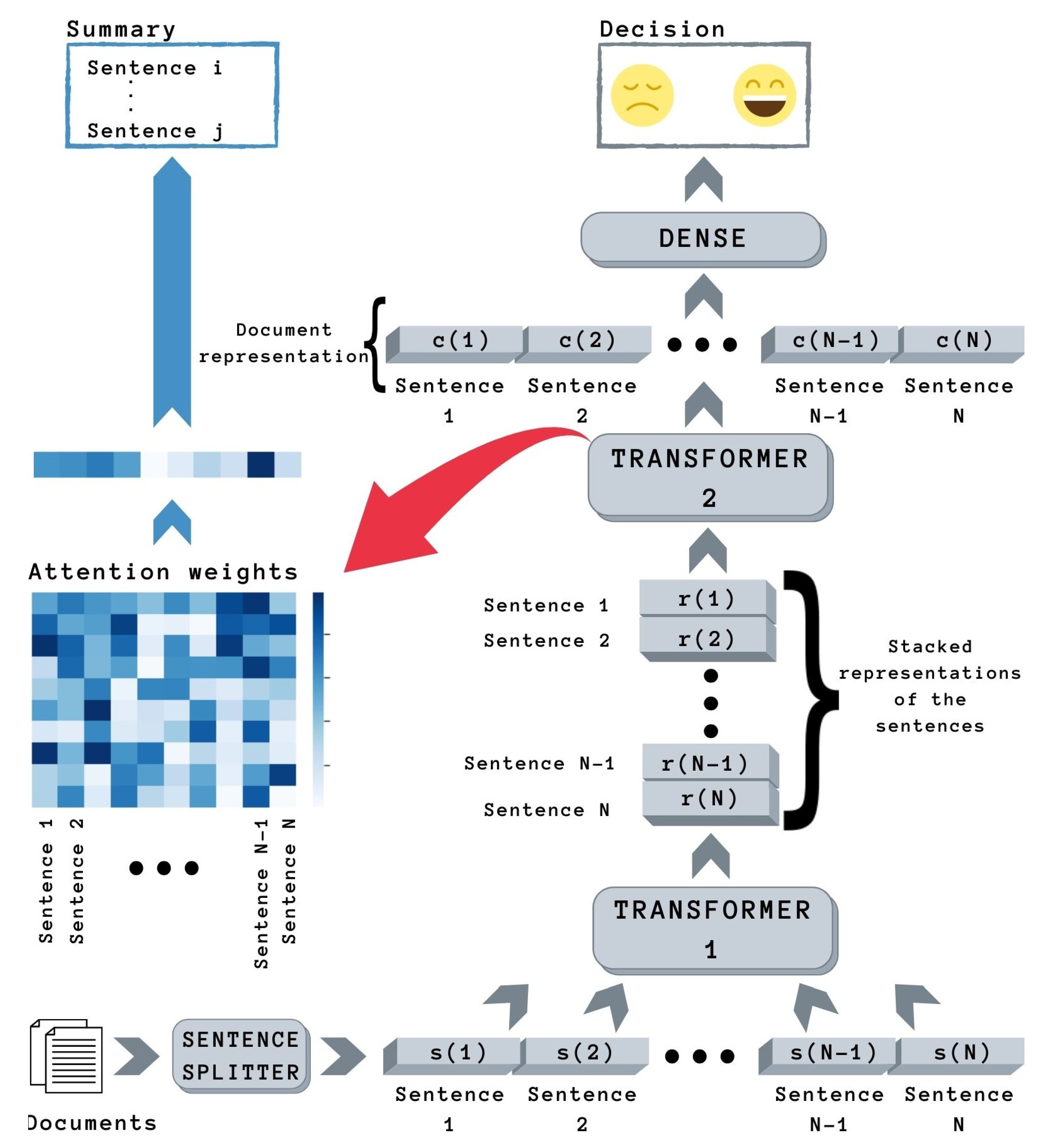
3.2.1. Explainable Hierarchical Transformer (ExHiT)

The first model exploits a hierarchical architecture, consisting of two transformers ($T1$ and $T2$) in cascade (Figure 1). Because of its nature, we like to refer at this as the ExplainableHierarchicalTransformer (ExHiT). The input of the first transformer is a sequence of t tokens, while the output is an embedding representation of that sequence. Each sequence represents one of the N sentences {$s_1\dots s_N$} in which the document is divided. If a document can be divided into just $m\le N$ sentences, then $N-m$ empty sentences (just the special tokens) are added to the document. After $T1$ has elaborated the N sequences, the new generated representations $\{r_1\dots r_N\}$ are stacked together to become the input of $T2$. $T2$ then outputs a contextual representation $c_i$ for the i-th sentence that depends on the other sentences ($c_i=f(r_1\dots r_N)$). By merging these contextual representations we obtain an unique document representation $d=U(c_1\dots c_N)$. In this work, we investigated the following merging strategies:

• By concatenation: $U(.)=Concat(.)$;
• By averaging: $U(.)=Avg(.)$;
• By masked averaging: $U(c_1\dots c_N)=Avg(c_1\dots c_m)$ with $m\le N$, for which $\{s_{m+1}\dots s_N\}$ is the set of the added empty sentences;
• By the application of a Bidirectional LSTM: $U(.)=BiLSTM(.)$.

Then, vector d is given as input to a classification layer. In this work, such a layer consists of a two-units fully-connected dense layer with the softmax activation for the binary classification task. Other than the contextual representations, we were able to retrieve from $T2$ also the self-attention weights for each head of each layer inside the transformer itself. To give more importance to the interpretability of the model instead of the performance, $T2$ consists only of two layers and just one head per layer. In this way, it is easier to extract valuable information. By averaging the attention weights associated with a specific sentence, we extracted the score of that sentence. The sentences are ranked through such a score, and the most important ones are then selected to provide an extractive summary of the document. Such a summary serves then as the explanation of the model decision.

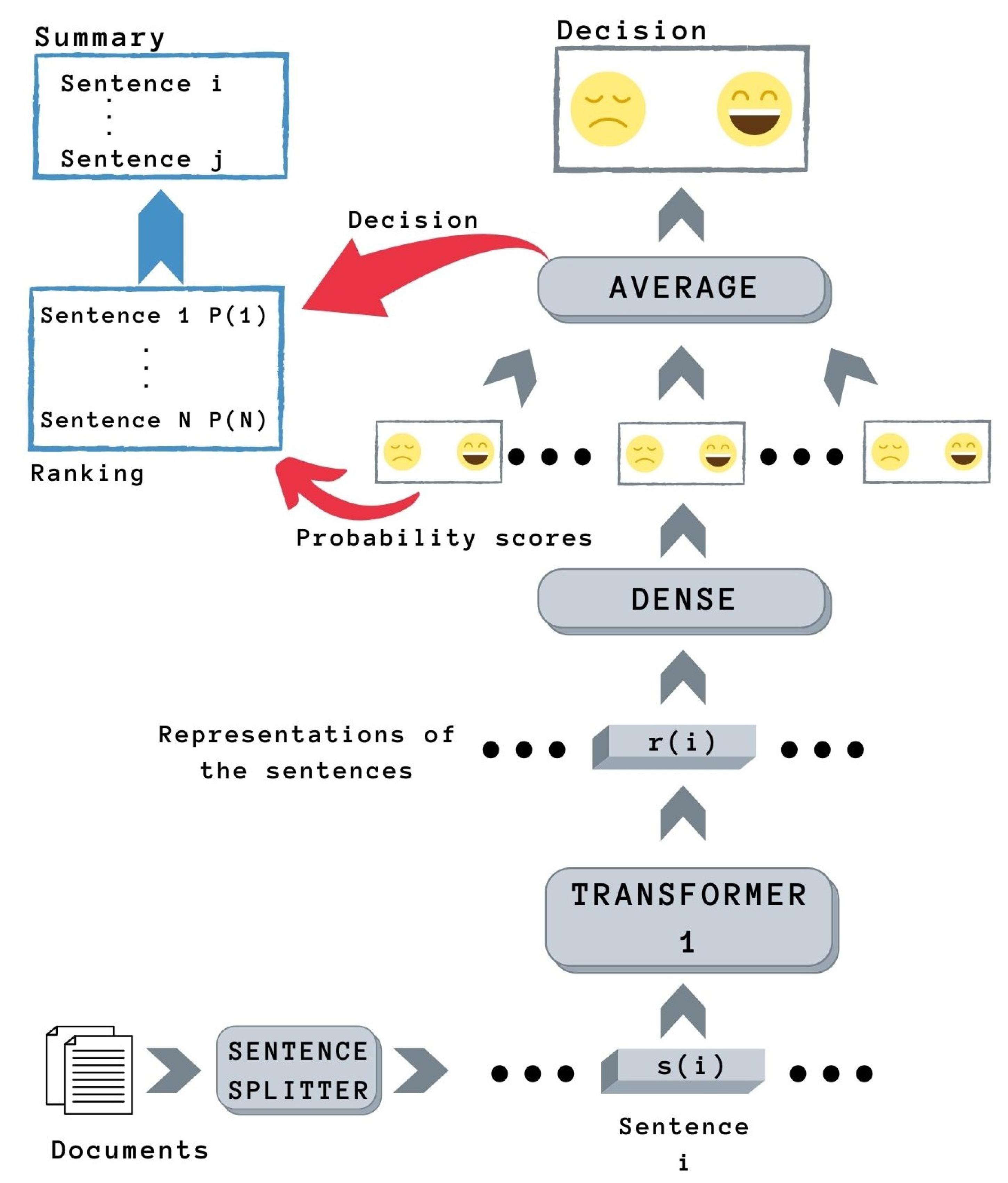
3.2.2. Sentence Classification Combiner Model (SCC)

This second model has a simpler architecture (Figure 2), requiring just one transformer model in its pipeline. The input of this transformer is again a sequence of t tokens, i.e., the single sentence $s_i$. Again, its output is a new representation $r_i$ of that sentence. Such representation is given in input to a dense layer to classify the sentiment of the sentence, outputting two probability scores, one for each class. Then, the negative scores are averaged together, and the same for the positive ones, to get a final rating for each class. The prediction of the overall document sentiment will be given by whoever has the greatest final score. Knowing the decision of the model, the sentences are ranked by the inherent probability score. Then, the most relevant ones are extracted to build the summary of the document, serving as an explanation of the model decision.

3.2.3. Parameters

In the following, we listed the main features of the two models used in the experiment’s session:

• T1: For a fair comparison, the first transformer model was the same for both the architectures; we opted to use the pre-trained version of RoBERTa [36];
• T2: We used a transformer with two layers, one head per layer; this choice was motivated to facilitate the explainability phase;
• N: The maximum number of sentences per document was set to 15; by this way, we ensured that the 75% of the training documents were elaborated in their entirety;
• t: The maximum number of tokens per sentence was set to 32, comprehensive of the two special delimiter tokens; by this way, we ensured that the 75% of the training sentences were elaborated without being truncated.

In addition to the two models, we implemented a pre-processing phase consisting of the replacement of the tokens ’<\br><\br>’ with the newline character, and, obviously, a sentence splitting step. We used the sentence tokenizer provided by NLTK. Furthermore, for documents that do not reach N number of sentences, empty sentences (consisting of just the special tokens) were added up to N. Similar reasoning was applied to sentences that do not reach the t number of tokens: in these cases, the sequences were zero-padded on the right, and an attention mask was applied.

4. Experiments

The SCC model was trained on the single sentence classification task, with a batch size of 240 sequences. Thus, the transformer together with the dense layer has been trained to classify the sentiment of every single sentence. After that, the average layer has been added on top of the trained model to perform the document classification (and its explanation) in the test phase. For what concerns the ExHiT model, the experiments followed two different fashions, always maintaining a batch size of 8 documents.

4.1. Joint Training

In this kind of experiment, the entire model was jointly trained on the document classification task. In this conceptualization, the weights of both the two transformers, the dense layer and, eventually, the merging layer (BiLSTM) were allowed to be updated during the training phase.

4.2. Ablation Study

In this kind of study, a model is modified by adding or removing some features from its architecture. In a first experiment, we added to the model the following features:

• Sinusoidal sentence positional embedding for T2 (SPE): following the original works on the transformers architectures, we added the positional embedding to the sentence embedding in input to the second transformer;
• Sentence masking for T2 (SM): following the principle of the attention mask for the padded token of the sequences in input to the first transformer, we applied an attention mask on the empty sentences added at the bottom of the document.

These two items were added under the hypothesis that encoding the relative position between the sentences and masking the empty sentences may improve the model performance. In a second experiment, we froze the weights from the first transformer also during the training. This experiment was conducted to investigate the following hypothesis: by freezing its weights, no knowledge can be learned by T1 during the training phase; thus, this configuration should force the second transformer to learn the most important features from the document to perform the task it is trained for. Even if it could lead to degradation in the sentiment classification performance, if this assumption was confirmed, it could potentially lead to improving the explanation performances.

The ablation study experiments were conducted using the ExHiT model implementing the concatenation merging strategy.

5. Results

The proposed models were evaluated for both sentiment analysis and explainability outcomes. In Table 1, we reported the sentiment analysis results achieved in terms of accuracy, and precision, recall, and F1-score per class. For the ExHiT model, various proposed merging strategies were tested. As the accuracy column highlights, changing the merging strategy does not significantly affects classification performance.

Table 1. Sentiment analysis results in terms of accuracy, and precision, recall, and F1-score per class.

Model	Merging Strategy	Accuracy (%)	Precision (%)		Recall (%)		F1 (%)
			Neg	Pos	Neg	Pos	Neg	Pos
ExHiT	Concatenation	92.59	90.97	94.34	94.56	90.62	92.73	92.44
	Average	92.35	92.18	92.51	92.54	92.15	92.36	92.33
	Masked Average	92.77	92.07	93.49	93.60	91.94	92.83	92.71
	BiLSTM	92.34	90.97	93.80	94.01	90.67	92.47	93.06
SCC	-	93.51	95.42	91.75	91.40	95.62	93.37	93.65

Following the same structure, in Table 2 we reported the explainability outcomes in terms of precision averaged over all the documents. The performances are reported for different annotators’ agreements, i.e., we built summaries by grouping the sentences for which at least one, two, or three out of the four annotators judged them among the most important ones. This implies that some annotators’ summaries of the j-th document may contain more than three sentences ($N_j>3$, especially in the first case) or less than three sentences ($N_j<3$, especially in the latter case). Therefore, we extracted the first $N_j$ sentences in the machine’s ranking and evaluated the overlap of these summaries with the annotators’ ones. The formula of the introduced explainability metric is reported in Equation (2):

$$Precision=\frac{1}{D}\sum _j^D\frac{T{P}_j}{N_j}\in [0,1]$$

(2)

where D is the number of documents, $N_j$ is the number of sentences in the annotators’ summary, and $T{P}_j$ is the number of well-selected sentences in the system summary of the j-th document. Documents for which $N_j$ was equal to 0 were excluded from the computation. This may happen, in particular, where an agreement of at least three annotators was required. About the ExHiT performance, the results of the best layer are reported. In general, the ranking from the first layer slightly outperformed the rankings from the last layer and the rankings obtained by averaging both layers. Furthermore, the empty sentences were removed by the machine rankings.

Table 2. Explainability performance in terms of precision (averaged over all documents) for different annotators agreements, evaluated on both the annotated documents from training and test sets. For ExHiT model the performances from the first layer are reported, except when the rankings from the last layer ¹ or from the average of layers ^a have shown better results.

Model	Merging Strategy	Agreement at Least 1		Agreement at Least 2		Agreement at Least 3
		Precision (%)		Precision (%)		Precision (%)
		Test	Train	Test	Train	Test	Train
ExHiT	Concatenation	53.82%	55.88% a	49.15%	45.00%	46.63%	46.45%
	Average	58.04%	57.82%	50.42%	45.92% 1	45.29%	41.84%
	Masked Average	53.15% a	55.79%	45.97% a	44.92%	40.66%	39.80%
	BiLSTM	55.51% a	55.85%	49.05% a	45.24% a	43.38% a	39.95%
SCC	-	70.74%	65.61%	65.22%	57.83%	55.22%	47.52%

For what concerns the ablation study on the ExHiT model, we combined the configurations described in Section 4.2, exploiting only the concatenation merging strategy. We reported the results of these experiments in Table 3, both in terms of accuracy and explainability precision. Again, the explainability performances are related with the first layer in general, except when the last layer or an average between both presents (slightly) better summaries. However, in the models implementing the sentence masking for the second transformer we found out a greater degree of agreement between the layers, and it was not rare to see the precision scores from the first layer only slight higher than the scores retrieved from the last layer (or the scores obtained by averaging the attention weights from both layers).

Table 3. Ablation study outcomes for the ExHiT model, both in terms of accuracy and explainability precision. SM stands for sentence masking, SPE stands for sentence positional embeddings. Frozen T1 indicates that the the weights of T1 were frozen during the training. The model is intended to implement the concatenation merging strategy. As in Table 2, results from the last layer or from the average of layers are indicated with the apices ¹ and ^a, respectively. Otherwise, the reported results are intended to be related with the first layer.

Model	Accuracy (%)	Agreement at Least 1		Agreement at Least 2		Agreement at Least 3
		Precision (%)		Precision (%)		Precision (%)
		Test	Train	Test	Train	Test	Train
ExHiT	92.59%	53.82%	55.88% a	49.15%	45.00%	46.63%	46.45%
+ SM	92.51%	67.24%	68.27%	59.82%	56.17%	54.88%	57.09% a
+ SPE	92.37%	64.34%	65.35%	58.13%	56.33%	52.19%	56.38%
+ SM + SPE	92.67%	70.27% a	69.11% 1	63.65%	63.50%	55.56%	55.67% a
Frozen T1	89.50%	63.43%	68.16% a	52.78% a	56.00%	44.11% a	48.23% a
SCC	93.51%	70.74%	65.61%	65.22%	57.83%	55.22%	47.52%

In Table 2 and Table 3, we compared the different models’ explainability with what we may call the explainability precision. Such a metric may take place with a priori annotations, i.e., the annotations are made on the original documents. To conduct a more in-depth analysis on the explainability error, we are also proposing a new metric that takes advantage of a posteriori annotations, i.e., the annotations are made on the (N=) 3-sentences summaries retrieved by each model. Here, the annotators were instructed to annotate each sentence as (1), negative (−1) or neutral (0) depending on the polarity of the document it lets them understand. The final score of the model exploits a sort of mean absolute error (MAE) for discrete variables. Hence, the total score is computed by following Equation (3)

$$1-\frac{1}{2}MAE=1-\frac{1}{2D}\sum _j^D\frac{1}{N_j}\sum _i^{N_j}|c_j-s_{j,i}|\in [0,1]$$

(3)

where D is the number of documents, N is the number of sentences per summary, $c_j$ is the predicted class of the j-th document, and $s_{j,i}$ is the annotated score of the i-th sentence (of the j-th document), and $\frac{1}{2}$ is a corrective factor to map the range of the MAE function (and, therefore, of the score) into an interval of $[0,1]$. In particular, in our case we fixed $N_j$ to be equal to $N=3$, also excluding the documents with less than 3 sentences from the computation of the total score). In this case, the previous equation may be rewritten in the form of the following equation:

$$1-\frac{1}{2}MAE=1-\frac{1}{2DN}\sum _j^D\sum _i^N|c_j-s_{j,i}|\in [0,1]$$

(4)

The contribution of each sentence $-\frac{1}{2}|c_j-s_{j,i}|$ to the total score is, therefore, equal to 0 if the prediction and the sentence score belong to the same class, −1 if they belong to opposite classes, and $-\frac{1}{2}$ if the sentence is annotated as neutral. Thus, the total score is a real number that lies in the range between 0 (dramatic extreme case, in which all the sentences belongs to the class opposite of the prediction) and 1 (desirable extreme case, in which all sentences belongs to the same class of the prediction). In particular, if the score is equal to $\frac{1}{2}$, it means that all the extracted sentences are evaluated as neutral by the humans (or that the number of well-ranked sentences counterbalances the number of the sentences classified as belonging to the class opposite of the prediction). Thus:

• If $1-\frac{1}{2}MAE<\frac{1}{2}\Rightarrow$ the model performance is worst than if it chose all neutral sentences;
• If $1-\frac{1}{2}MAE>\frac{1}{2}\Rightarrow$ the model is going better than if it chose all neutral sentences.

To avoid any bias for the annotators deriving from the prediction of the model or from the other sentences of the document, the predicted class was obscured and the sentences of all the documents were shuffled together. The annotations were performed just for three of the models trained in this work, as reported in Table 4. In particular, the results about the ExHiT-based systems come from the attention head of the first layer of the second transformer.

Table 4. Explainability performance in terms of the proposed score, reported in Equation (4), and percentage of summary’s sentences annotated as neutral. The ExHiT models are intended to be implemented with the concatenation merging strategy, and the summaries built by the first layer are analyzed.

Model	$1-\frac{1}{2}\mathbf{MAE}$ (%)		Neutral Rate (%)
	Test	Train	Test	Train
ExHiT	78.33%	74.67%	26.00%	35.37%
+ SM + SPE	86.50%	82.67%	13.00%	17.69%
SCC	92.67%	88.67%	11.56%	19.05%

6. Discussion

By analyzing Table 1, the SCC model seems to achieve a slightly better overall performance. However, it is interesting to notice that SCC results are particularly good for the precision for the negative class and the recall for the positive one while achieving the worst performances for their counterpart metrics, for which the best results are obtained by ExHiT using the concatenation merging strategy. About Table 2, the ExHiT explainability results are lower than those achieved by SCC, with respect to all the merging strategies. This outcome may be due to an influence of the task on the two models: it may be noticed that the task the second model accomplishes is closer to the one performed by the annotators. It may, therefore, help the SCC model in the explainability task. Furthermore, the average merging strategy leads to better performance than the masked one, especially with respect to the test set (∼+5%). This seems to suggest that masking the empty sentences from the average combination after the elaboration of the second transformer does not help the model to better understand the task.

For what concerns the ablation study conducted in this work, the obtained results are very interesting (Table 3), in particular, for what regards the explainability performance. In fact, while the sentiment classification did not show significant improvements in terms of accuracy, ExHiT models implementing the empty sentence masking have shown significant improvements in terms of explainability precision, achieving results comparable with the SCC model. In some cases, it reaches even better outcomes, especially when it is combined with the introduction of the sinusoidal sentence position embeddings, a strategy that has shown explainability improvements even when implemented alone. Furthermore, exploiting a qualitative analysis of the outcomes of the various models, it has been observed how the ExHiT-based systems “suffer” from the noisy empty sentences added to achieve the maximum number of the sentence required by the architecture, with the exception of the models implementing the sentence mask. This behavior is highlighted in Table 5, reporting the sentences from the same document ranked by two ExHiT models, one not implementing the sentence mask and one that does it, respectively. In the example reported here, it is easy to notice the presence of the empty sentences among the first positions of the ranking built by the former, while they are always ignored by the latter model itself and thus put on the bottom part of the constructed ranking.

Table 5. Example of document summary generated by two ExHiT models, one implementing sentence masking (right) and the other without the sentence mask (left). The index columns indicate the position of each sentence in the original document.

Index	ExHiT	Index	ExHiT + SM
0	This film was a surprise.	0	This film was a surprise.
6	Jealousy, sexual tension, incest, intrigue, […]	6	Jealousy, sexual tension, incest, intrigue, […]
11	Even though her strength and lack of illusion […]	1	The plot synopsis sounds kinky […]
13		8	However, I wanted to clarify a point […]
14		10	The attractive female slave successfully resists […]
4	The child takes him to the girls […]	9	I find that there is one.
10	The attractive female slave successfully resists […]	3	There is that opening scene where […]
3	There is that opening scene where […]	11	Even though her strength and lack of illusion […]
5	He takes advantage of the situation […]	2	I didn’t know what to expect.
7	I’ve read the other comments here and find little to disagree with.	5	He takes advantage of the situation […]
2	I didn’t know what to expect.	7	I’ve read the other comments here and find little to disagree with.
12	She, more than any of the other women […]	4	The child takes him to the girls […]
9	I find that there is one.	12	She, more than any of the other women […]
8	However, I wanted to clarify a point […]	13
1	The plot synopsis sounds kinky […]	14

These considerations seem to suggest that the sentence mask is essential to filter out the noisy empty sentences and, therefore, better understand the task. However, with or without sentence masking, the performances of the classification task of the two kinds of models are not so far from each other. Thus, we hypothesized that, in absence of the sentence masking, the model captures other kinds of information from the text and learns how to use them to perform the sentiment analysis task. Exploiting these features thus leads to good performance in the main task, but being inherently less interpretable for humans it is inevitable for the model to reach worse explainability performance.

The performed ablation study reports interesting results when T1 weights are frozen during the training phase. In this case, the model has shown good improvements in terms of explainability precision. This seems to confirm our hypothesis that freezing the first transformer prevents it from adapting to the task during training and then forces the second transformer to boost its ability to extract important information from the sentences. In fact, the results in Table 3 show that this trick can in part compensate for the absence of sentence masking, at the cost of ∼3 percentage points on the classification accuracy.

For what concerns explainability, in Table 4 results in terms of MAE are reported for some models. We proposed this kind of metric after visualizing models’ outcomes. Figure 3 shows an example of document annotation performed by the annotators, in which darker background means higher relevance in the document, computed as the average of agreement among the annotators. Figure 4 shows the annotations performed by the SCC model on the same example. Again, darker background means higher relevance, in this case in terms of the probability scores.

Figure 3. Example of document annotation performed (a priori) by the instructed annotators.

Figure 4. Example of document annotation performed by the SCC model during the classification.

As it can be seen, if we consider the case of agreement of at least three out of the four annotators, the explainability precision would be null. In fact, the annotators’ summary would be built by extracting the sentences numbered as {1, 3, and 4} while the model’s summary would consist of the sentences numbered as {5, 6, and 9}. However, at a further analysis, it seems clear that the second set of sentences contain a negative sentiment, as well as the first set. Thus, the introduction of such a posteriori metric was necessary to perform a fairer comparison between the models. Unfortunately, being a posteriori metric brings the drawback to perform human annotations on the outcomes of each model we want to compare. For this reason, this analysis was limited only to three of the developed models. The outcomes in terms of this metric (Table 4) still show the SCC model to outperform the other(s). Very interestingly, for the test dataset, it achieves a very high score, greater than 92%. This seems to suggest that this model not only can achieve a near state-of-the-art accuracy in the sentiment analysis task but also provides a very accurate extractive summary as an explanation of the predicted class. However, to compute this metric the introduction of a new class, the neutral one, was necessary to perform the annotations. The reason is, of course, we cannot exclude a priori that some summary extracted from the template may contain uninformative sentences with respect to the sentiment of the full review. In particular, for both kinds of models, many of the sentences classified by annotators as neutral are excerpts of plot narration. For example, the sentence

But success has it’s downside, as Macbeth soon finds out, when he has to go to hideous lengths to protect his murderous secret.

is simply a description of a plot passage in the movie Macbeth—The tragedy of ambition and contains no information about the sentiment of the review provided by the user and, therefore, would be impossible for an annotator to classify as black or white. Another kind of sentence extracted by the models is sentences that may gain a sentiment sense only if seen together with the previous or next parts of the document. For example, the sentence

You’ll be glad you did.

has no particular sentiment when picked alone and gives no clue about the polarity of the document. In fact, it is licit for an annotator to wonder: I’ll be glad I did what?. Thus, this sentence alone does not give good hints to guess the sentiment nature of the document. However, if you look at this sentence inside its context

Do yourself a favor and avoid this movie at all costs. You’ll be glad you did.

it can be easily noticed that it enforces the negative sense of the previous part of the discourse. The annotators reported this kind of behavior for the ExHiT model, in particular, and this seems to be confirmed by the last two columns of Table 4, where a greater percentage of neutral annotations is reported for both training and test set with respect to the SCC model. This seems to suggest that the ExHiT model it is less suited to perform single sentence-extractive summaries, because of a more contextual understanding of the document classification task. However, the ExHiT version implementing both the sentence masking and positional embeddings has been reported to less show this behavior. In fact, its neutral percentage is way lower than the simpler version. In the case of the training set, it is even lower than the SCC system. Furthermore, also the proposed score presents a significant improvement. These outcomes suggest, once again, how these components are of great importance to the interpretability of the hierarchical model.

7. Conclusions

In this work, we proposed two transformer-based architectures to perform a task of (document) sentiment analysis classification while also providing an extractive summary of the classified document as an explanation of the model decision. These architectures were designed to exploit the inherent hierarchy of documents, with the lower part of the model consisting of a transformer working at the intra-sentence tokens level, and the higher part working at the inter-sentences level. In the ExHiT case, the higher part consists of another transformer, one layer implementing some merging strategy, and a classifier layer. In the SCC case, the higher part just consists of an averaging layer to provide the document classification by averaging the classification scores of the single sentences constituting the whole text. For both models, the summary is built by extracting the original sentences from the document. The extraction phase takes place after ranking those sentences depending on the scores intrinsically computed by the two models. In the former case, we exploited the self-attention weights of the second transformer to produce those rankings, in the latter we used the probability scores assigned by the lower part of the system to the single sentences. To evaluate the built summaries, we proposed two metrics. However, by comparing the explainability results in Table 3 and Table 4, the tested models seem to share the same behavior with regard to both the proposed explainability metrics. Therefore, although being less fairer to the models themselves, it would not be wrong to prefer the precision metric over the other one to compare the explainability of different systems.

To the best of our knowledge, this is the first attempt to build a document classification paradigm of models that generate an extractive summary in order to provide an easy to interpret explanation to the user. Therefore, such models may be implemented in the near future in some industrial applications, such as customer care or market research tools. Both the proposed models have, in fact, achieved good classification results, not so far from the works at the state-of-the-art on the IMDB dataset, while also performing an explanation in the form of a summary. The explainability component of the models, achieving good results, as well as the classification one, is a feature that may become essential in several applications. For example, while sentiment analysis may help to mark customer messages and reviews, the explainability part may be helpful to get quick insights about the strengths and the weaknesses of some product or service. Furthermore, both underlying architectures allow their easy adaptation in any document classification task (e.g., topic classification). Plus, both models may be applied to any language: the only restriction is to use the suitable pre-trained model as T1, i.e., a transformer model that has been pre-trained on the task language (or, at least, in a multilingual fashion). This is an interesting point of view for the next research works to focus on. Sentiment analysis is, in fact, a task that particularly relies on the lexical meaning of the individual sentences. Therefore, evaluating our models on a different kind of task may show ExHiT outperforming the SCC model because of its ability to get more insights from the context of the other sentences in the document. In particular, since both models hide the potential to be able to operate on tasks involving longer documents, which is a sort of limitation for traditional transformer architectures, it would be very interesting to study if they can overcome such a limit by applying them to tasks requiring large documents, say several hundreds of tokens (or even more!). Another attractive idea to follow is to go in-depth with the analyses in the ablation study for the ExHiT architecture. We have shown how masking the empty sentences and adding the positional embedding may play an important role for the model, and how freezing the first transformer during training may force the higher part to learn more interpretable features. Future research may extend this kind of study by evaluating the performance (both in terms of classification and explainability) achieved by deeper models, e.g., adding more layers and self-attention heads to the second transformer. To conclude, the explainability at a finer granularity (the tokens level) may be explored by investigating the attention weights of the first transformer for both kinds of architectures, e.g., by highlighting the most important words in each sentence.

References

1. Dashtipour, K.; Gogate, M.; Cambria, E.; Hussain, A. A novel context-aware multimodal framework for persian sentiment analysis. arXiv 2021, arXiv:2103.02636. [Google Scholar]
2. Gunning, D. Explainable Artificial Intelligence (XAI); Defense Advanced Research Projects Agency (DARPA): Arlington County, VA, USA, 2017. [Google Scholar]
3. Gunning, D.; Aha, D. DARPA’s explainable artificial intelligence (XAI) program. AI Mag. 2019, 40, 44–58. [Google Scholar]
4. Arrieta, A.B.; Díaz-Rodríguez, N.; Del Ser, J.; Bennetot, A.; Tabik, S.; Barbado, A.; García, S.; Gil-López, S.; Molina, D.; Benjamins, R.; et al. Explainable Artificial Intelligence (XAI): Concepts, taxonomies, opportunities and challenges toward responsible AI. Inf. Fusion 2020, 58, 82–115. [Google Scholar] [CrossRef] [Green Version]
5. Loyola-Gonzalez, O. Black-box vs. white-box: Understanding their advantages and weaknesses from a practical point of view. IEEE Access 2019, 7, 154096–154113. [Google Scholar] [CrossRef]
6. Danilevsky, M.; Qian, K.; Aharonov, R.; Katsis, Y.; Kawas, B.; Sen, P. A survey of the state of explainable AI for natural language processing. arXiv 2020, arXiv:2010.00711. [Google Scholar]
7. Vaswani, A.; Shazeer, N.; Parmar, N.; Uszkoreit, J.; Jones, L.; Gomez, A.N.; Kaiser, Ł.; Polosukhin, I. Attention is all you need. In Proceedings of the Advances in Neural Information Processing Systems, Long Beach, CA, USA, 4–9 December 2017. [Google Scholar]
8. Maas, A.; Daly, R.E.; Pham, P.T.; Huang, D.; Ng, A.Y.; Potts, C. Learning word vectors for sentiment analysis. In Proceedings of the 49th Annual Meeting of the Association for Computational Linguistics: Human Language Technologies, Portland, Oregon, 19–24 June 2011; pp. 142–150. [Google Scholar]
9. Liu, B. Sentiment analysis and opinion mining. Synth. Lect. Hum. Lang. Technol. 2012, 5, 1–167. [Google Scholar] [CrossRef] [Green Version]
10. McGlohon, M.; Glance, N.; Reiter, Z. Star quality: Aggregating reviews to rank products and merchants. In Proceedings of the Fourth International AAAI Conference on Weblogs and Social Media, Washington, DC, USA, 23–26 May 2010. [Google Scholar]
11. Zarzour, H.; Al shboul, B.; Al-Ayyoub, M.; Jararweh, Y. Sentiment Analysis Based on Deep Learning Methods for Explainable Recommendations with Reviews. In Proceedings of the 2021 12th International Conference on Information and Communication Systems (ICICS), Valencia, Spain, 24–26 May 2021; pp. 452–456. [Google Scholar]
12. Gite, S.; Khatavkar, H.; Kotecha, K.; Srivastava, S.; Maheshwari, P.; Pandey, N. Explainable stock prices prediction from financial news articles using sentiment analysis. PeerJ Comput. Sci. 2021, 7, e340. [Google Scholar] [CrossRef]
13. Joshi, M.; Das, D.; Gimpel, K.; Smith, N.A. Movie reviews and revenues: An experiment in text regression. In Proceedings of the Human Language Technologies: The 2010 Annual Conference of the North American Chapter of the Association for Computational Linguistics, Los Angeles, CA, USA, 2–4 June 2010; pp. 293–296. [Google Scholar]
14. Hu, M.; Liu, B. Mining opinion features in customer reviews. AAAI 2004, 4, 755–760. [Google Scholar]
15. Silveira, T.D.S.; Uszkoreit, H.; Ai, R. Using Aspect-Based Analysis for Explainable Sentiment Predictions. In Proceedings of the CCF International Conference on Natural Language Processing and Chinese Computing, Zhengzhou, China, 14–18 October 2019. [Google Scholar]
16. Baccianella, S.; Esuli, A.; Sebastiani, F. Sentiwordnet 3.0: An enhanced lexical resource for sentiment analysis and opinion mining. In Proceedings of the International Conference on Language Resources and Evaluation, LREC 2010, Valletta, Malta, 17–23 May 2010. [Google Scholar]
17. Cambria, E.; Speer, R.; Havasi, C.; Hussain, A. Senticnet: A publicly available semantic resource for opinion mining. In Proceedings of the AAAI Fall Symposium: Commonsense Knowledge, Arlington, VA, USA, 11–13 November 2010. [Google Scholar]
18. Zhang, Y.; Lai, G.; Zhang, M.; Zhang, Y.; Liu, Y.; Ma, S. Explicit factor models for explainable recommendation based on phrase-level sentiment analysis. In Proceedings of the 37th International Acm Sigir Conference on Research & Development in Information Retrieval, Gold Coast, Australia, 6–11 July 2014. [Google Scholar]
19. Zhao, A.; Yu, Y. Knowledge-enabled BERT for aspect-based sentiment analysis. Knowl. Based Syst. 2021, 227, 107220. [Google Scholar] [CrossRef]
20. Bacco, L.; Cimino, A.; Dell’Orletta, F.; Merone, M. Extractive Summarization for Explainable Sentiment Analysis Using Transformers. 2021. Available online: https://openreview.net/pdf?id=xB1deFXLaF9 (accessed on 7 July 2021).
21. El-Kassas, W.S.; Salama, C.R.; Rafea, A.A.; Mohamed, H.K. Automatic text summarization: A comprehensive survey. Expert Syst. Appl. 2020, 165, 113679. [Google Scholar] [CrossRef]
22. Elman, J.L. Finding structure in time. Cogn. Sci. 1990, 14, 179–211. [Google Scholar] [CrossRef]
23. Schuster, M.; Paliwal, K.K. Bidirectional recurrent neural networks. IEEE Trans. Signal Process. 1997, 45, 2673–2681. [Google Scholar] [CrossRef] [Green Version]
24. Bengio, Y.; Simard, P.; Frasconi, P. Learning long-term dependencies with gradient descent is difficult. IEEE Trans. Neural Netw. 1994, 5, 157–166. [Google Scholar] [CrossRef]
25. Hochreiter, S.; Schmidhuber, J. Long short-term memory. Neural Comput. 1997, 9, 1735–1780. [Google Scholar] [CrossRef]
26. Cho, K.; Van Merriënboer, B.; Gulcehre, C.; Bahdanau, D.; Bougares, F.; Schwenk, H.; Bengio, Y. Learning phrase representations using RNN encoder-decoder for statistical machine translation. arXiv 2014, arXiv:1406.1078. [Google Scholar]
27. Sundermeyer, M.; Schlüter, R.; Ney, H. LSTM neural networks for language modeling. In Proceedings of the Thirteenth Annual Conference of the International Speech Communication Association, Portland, Oregon, 9–13 September 2012. [Google Scholar]
28. Sundermeyer, M.; Ney, H.; Schlüter, R. From feedforward to recurrent LSTM neural networks for language modeling. IEEE/ACM Trans. Audio Speech Lang. Process. 2015, 23, 517–529. [Google Scholar] [CrossRef]
29. Larochelle, H.; Hinton, G.E. Learning to combine foveal glimpses with a third-order boltzmann machine. In Proceedings of the Advances in Neural Information Processing Systems, Vancouver, BC, Canada, 6–9 December 2010. [Google Scholar]
30. Bahdanau, D.; Cho, K.; Bengio, Y. Neural machine translation by jointly learning to align and translate. arXiv 2014, arXiv:1409.0473. [Google Scholar]
31. Radford, A.; Narasimhan, K.; Salimans, T.; Sutskever, I. Improving Language Understanding by Generative Pre-Training. 2018. Available online: https://s3-us-west-2.amazonaws.com/openai-assets/research-covers/language-unsupervised/language_understanding_paper.pdf (accessed on 8 February 2021).
32. Radford, A.; Wu, J.; Child, R.; Luan, D.; Amodei, D.; Sutskever, I. Language Models are Unsupervised Multitask Learners. 2019. Available online: https://d4mucfpksywv.cloudfront.net/better-language-models/language_models_are_unsupervised_multitask_learners.pdf (accessed on 8 February 2021).
33. Brown, T.B.; Mann, B.; Ryder, N.; Subbiah, M.; Kaplan, J.; Dhariwal, P.; Neelakantan, A.; Shyam, P.; Sastry, G.; Askell, A.; et al. Language models are few-shot learners. arXiv 2020, arXiv:2005.14165. [Google Scholar]
34. Yang, Z.; Dai, Z.; Yang, Y.; Carbonell, J.; Salakhutdinov, R.R.; Le, Q.V. Xlnet: Generalized autoregressive pretraining for language understanding. In Proceedings of the Advances in Neural Information Processing Systems, Vancouver, BC, Canada, 8–14 December 2019. [Google Scholar]
35. Devlin, J.; Chang, M.W.; Lee, K.; Toutanova, K. Bert: Pre-training of deep bidirectional transformers for language understanding. arXiv 2018, arXiv:1810.04805. [Google Scholar]
36. Liu, Y.; Ott, M.; Goyal, N.; Du, J.; Joshi, M.; Chen, D.; Levy, O.; Lewis, M.; Zettlemoyer, L.; Stoyanov, V. Roberta: A robustly optimized bert pretraining approach. arXiv 2019, arXiv:1907.11692. [Google Scholar]
37. Sanh, V.; Debut, L.; Chaumond, J.; Wolf, T. DistilBERT, a distilled version of BERT: smaller, faster, cheaper and lighter. arXiv 2019, arXiv:1910.01108. [Google Scholar]
38. Wolf, T.; Chaumond, J.; Debut, L.; Sanh, V.; Delangue, C.; Moi, A.; Rush, A.M. Transformers: State-of-the-art natural language processing. In Proceedings of the 2020 Conference on Empirical Methods in Natural Language Processing: System Demonstrations, Stroudsburg, PA, USA, 16–20 November 2020. [Google Scholar]
39. Pan, S.J.; Yang, Q. A survey on transfer learning. IEEE Trans. Knowl. Data Eng. 2009, 22, 1345–1359. [Google Scholar] [CrossRef]
40. Wang, A.; Singh, A.; Michael, J.; Hill, F.; Levy, O.; Bowman, S.R. Glue: A multi-task benchmark and analysis platform for natural language understanding. arXiv 2018, arXiv:1804.07461. [Google Scholar]
41. Peters, M.E.; Neumann, M.; Iyyer, M.; Gardner, M.; Clark, C.; Lee, K.; Zettlemoyer, L. Deep contextualized word representations. arXiv 2018, arXiv:1802.05365. [Google Scholar]
42. Howard, J.; Ruder, S. Universal language model fine-tuning for text classification. arXiv 2018, arXiv:1801.06146. [Google Scholar]
43. Pappagari, R.; Zelasko, P.; Villalba, J.; Carmiel, Y.; Dehak, N. Hierarchical transformers for long document classification. In Proceedings of the 2019 IEEE Automatic Speech Recognition and Understanding Workshop (ASRU), Singapore, 14–18 December 2019. [Google Scholar]
44. Pelicon, A.; Pranjić, M.; Miljković, D.; Škrlj, B.; Pollak, S. Zero-shot learning for cross-lingual news sentiment classification. Appl. Sci. 2020, 10, 5993. [Google Scholar] [CrossRef]
45. Zhang, X.; Wei, F.; Zhou, M. HIBERT: Document level pre-training of hierarchical bidirectional transformers for document summarization. arXiv 2019, arXiv:1905.06566. [Google Scholar]
46. Xu, S.; Zhang, X.; Wu, Y.; Wei, F.; Zhou, M. Unsupervised Extractive Summarization by Pre-training Hierarchical Transformers. arXiv 2020, arXiv:2010.08242. [Google Scholar]
47. Vig, J. A multiscale visualization of attention in the transformer model. arXiv 2019, arXiv:1906.05714. [Google Scholar]
48. Kovaleva, O.; Romanov, A.; Rogers, A.; Rumshisky, A. Revealing the dark secrets of BERT. arXiv 2019, arXiv:1908.08593. [Google Scholar]
49. Voita, E.; Serdyukov, P.; Sennrich, R.; Titov, I. Context-aware neural machine translation learns anaphora resolution. arXiv 2018, arXiv:1805.10163. [Google Scholar]
50. Goldberg, Y. Assessing BERT’s syntactic abilities. arXiv 2019, arXiv:1901.05287. [Google Scholar]
51. Wolf, T. Some Additional Experiments Extending the Tech Report “Assessing BERTs Syntactic Abilities” by Yoav Goldberg. 2019. Available online: https://huggingface.co/bert-syntax/extending-bert-syntax.pdf (accessed on 5 February 2021).
52. Hewitt, J.; Manning, C.D. A structural probe for finding syntax in word representations. In Proceedings of the 2019 Conference of the North American Chapter of the Association for Computational Linguistics: Human Language Technologies, Minneapolis, MN, USA, 2–7 June 2019; Volume 1, pp. 4129–4138. [Google Scholar]
53. Raganato, A.; Tiedemann, J. An analysis of encoder representations in transformer-based machine translation. In Proceedings of the 2018 EMNLP Workshop BlackboxNLP: Analyzing and Interpreting Neural Networks for NLP, Brussels, Belgium, 1 November 2018. [Google Scholar]
54. Vig, J.; Belinkov, Y. Analyzing the structure of attention in a transformer language model. arXiv 2019, arXiv:1906.04284. [Google Scholar]
55. Voita, E.; Talbot, D.; Moiseev, F.; Sennrich, R.; Titov, I. Analyzing multi-head self-attention: Specialized heads do the heavy lifting, the rest can be pruned. arXiv 2019, arXiv:1905.09418. [Google Scholar]
56. Franz, L.; Shrestha, Y.R.; Paudel, B. A deep learning pipeline for patient diagnosis prediction using electronic health records. arXiv 2020, arXiv:2006.16926. [Google Scholar]
57. Letarte, G.; Paradis, F.; Giguère, P.; Laviolette, F. Importance of self-attention for sentiment analysis. In Proceedings of the 2018 EMNLP Workshop BlackboxNLP: Analyzing and Interpreting Neural Networks for NLP, Brussels, Belgium, 1 November 2018. [Google Scholar]
58. Bodria, F.; Panisson, A.; Perotti, A.; Piaggesi, S. Explainability Methods for Natural Language Processing: Applications to Sentiment Analysis (Discussion Paper). 2020. Available online: http://ceur-ws.org/Vol-2646/18-paper.pdf (accessed on 17 January 2021).
59. Ribeiro, M.T.; Singh, S.; Guestrin, C. “Why should i trust you?” Explaining the predictions of any classifier. In Proceedings of the 22nd ACM SIGKDD International Conference on Knowledge Discovery and Data Mining, San Francisco, CA, USA, 13–17 August 2016. [Google Scholar]
60. Zhang, Y.; Song, K.; Sun, Y.; Tan, S.; Udell, M. “Why Should You Trust My Explanation?” Understanding Uncertainty in LIME Explanations. arXiv 2019, arXiv:1904.12991. [Google Scholar]
61. Sundararajan, M.; Taly, A.; Yan, Q. Axiomatic attribution for deep networks. In Proceedings of the International Conference on Machine Learning, Sydney, Australia, 6–11 August 2017; pp. 3319–3328. [Google Scholar]
62. Krippendorff, K. Estimating the reliability, systematic error and random error of interval data. Educ. Psychol. Meas. 1970, 30, 61–70. [Google Scholar] [CrossRef]
63. Krippendorff, K. Content Analysis: An Introduction to Its Methodology, 2nd ed.; SAGE Publications, Inc.: Thousand Oaks, CA, USA, 2004. [Google Scholar]
64. Krippendorff, K. Reliability in content analysis: Some common misconceptions and recommendations. Hum. Commun. Res. 2004, 30, 411–433. [Google Scholar] [CrossRef]
Publisher’s Note: MDPI stays neutral with regard to jurisdictional claims in published maps and institutional affiliations.
Article Metrics
Citations
Article Access Statistics
Multiple requests from the same IP address are counted as one view.