
Towards Precision Fertilization: Multi-Strategy Grey Wolf Optimizer Based Model Evaluation and Yield Estimation

 ,
,  ,
,
Abstract
1. Introduction
2. Materials and Methods
2.1. GWO
2.2. Opposition-Based Learning
2.3. Slime Mould Foraging
2.4. Levy Flight
2.5. GS (Greedy Strategy)
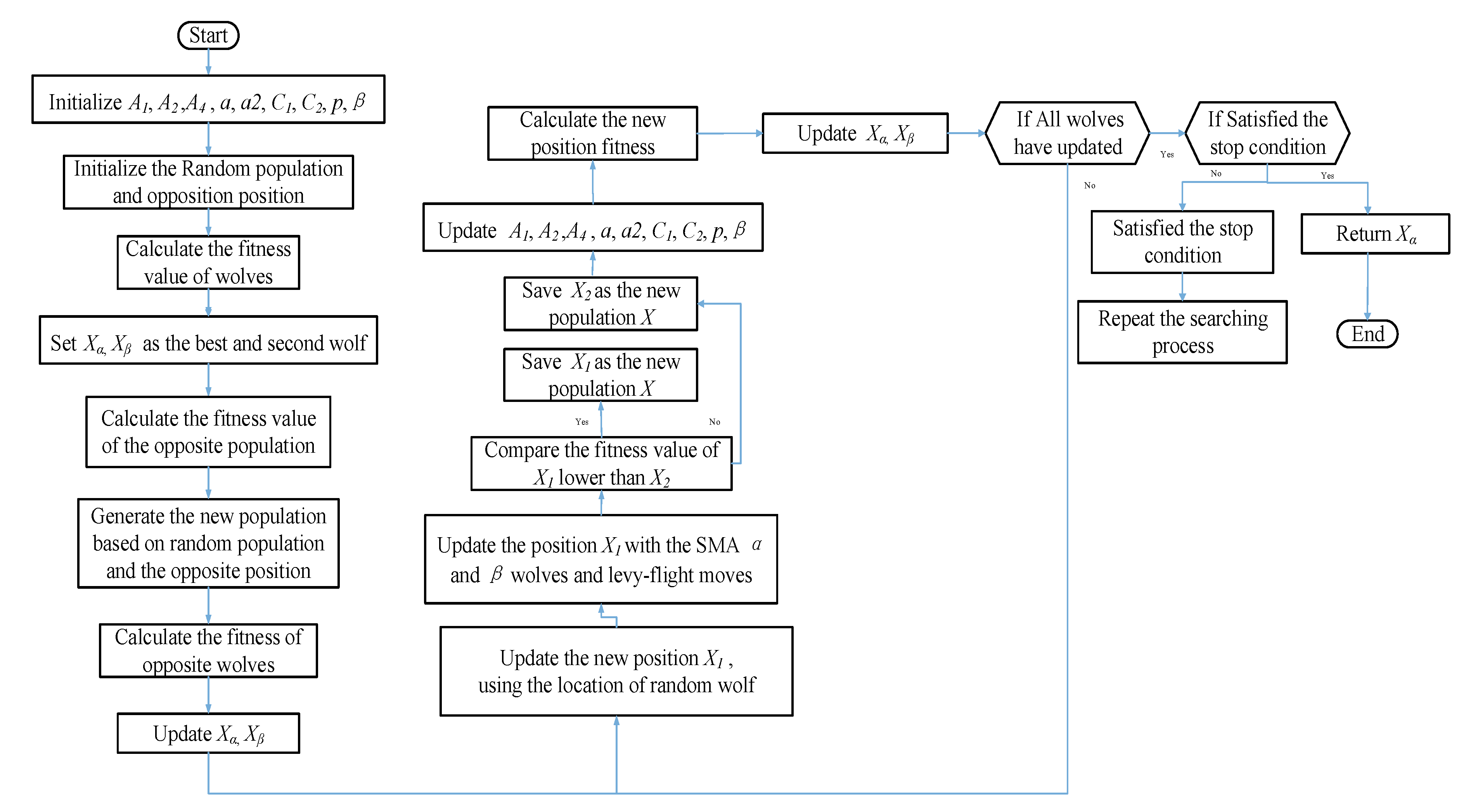
2.6. Multi-Strategy Grey Wolf Optimizer (SLEGWO)
3. Experiments and Results for Benchmark Function
3.1. Benchmark Function Validation
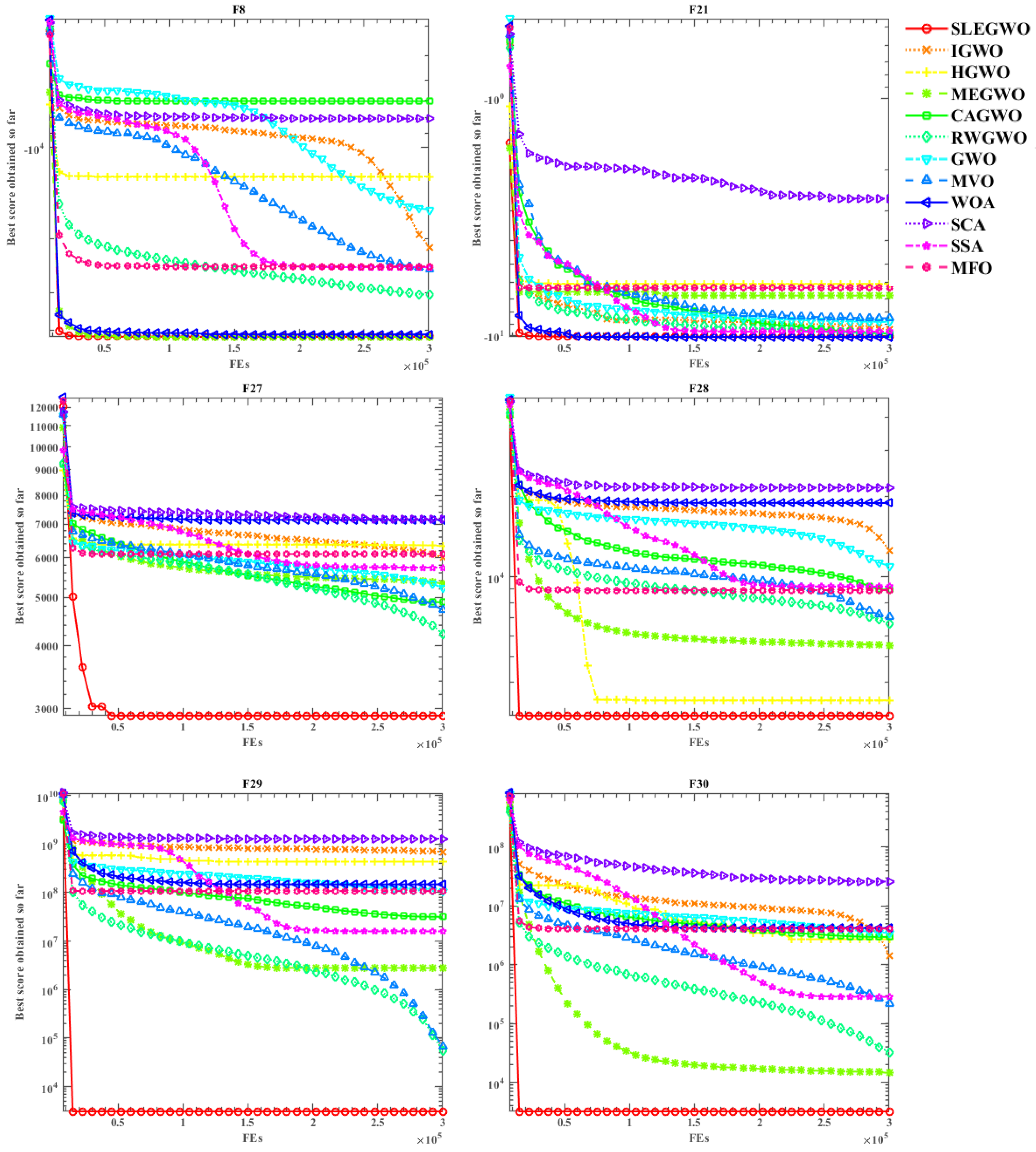
3.2. Comparison with Competitive Algorithms
4. SLEGWO Precision Fertilization Model
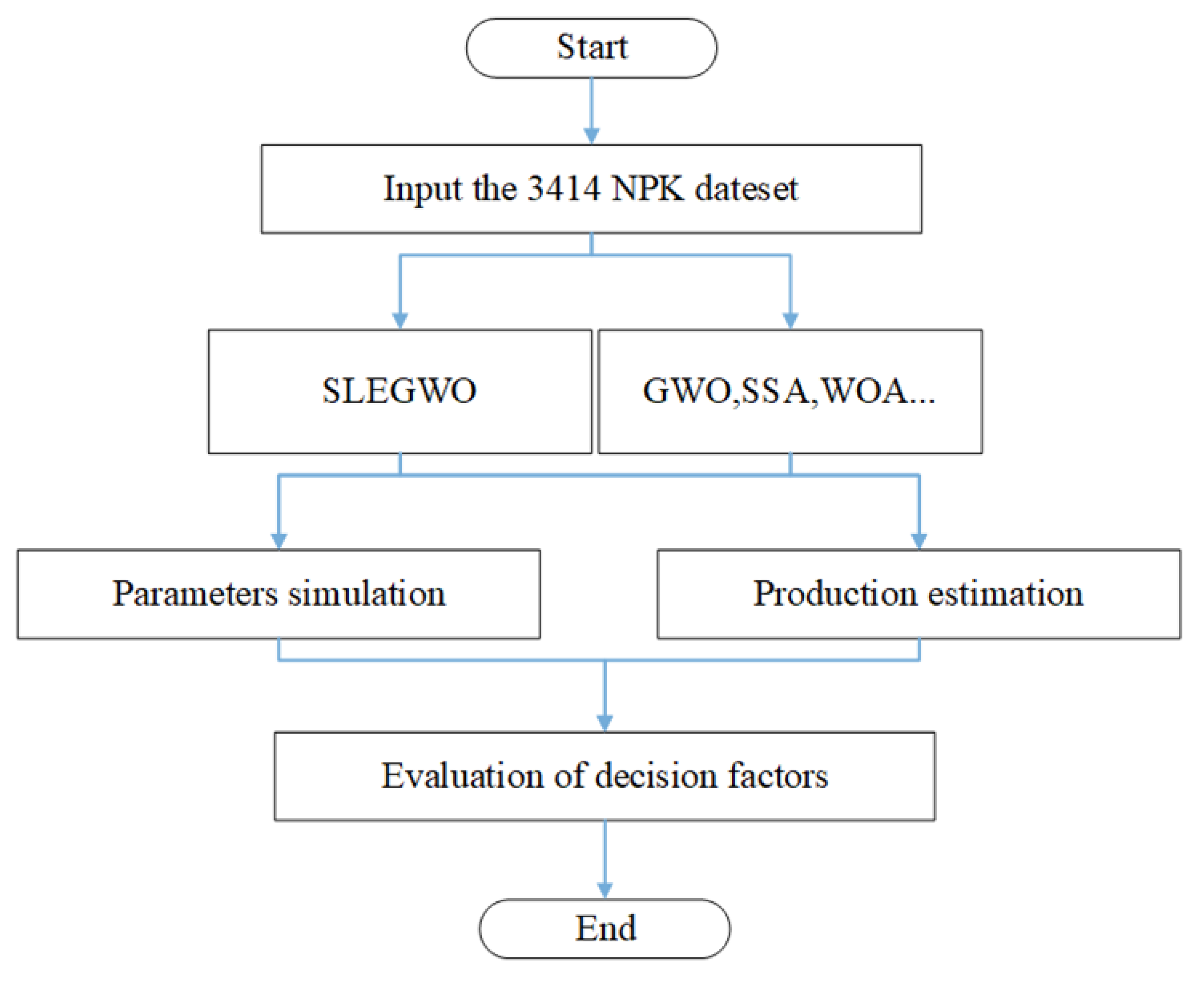
4.1. SLEGWO and NPK Precision Fertilization Method
4.2. Experimental Environment
4.3. Experimental Dataset
4.4. Solution of Equation Coefficients
4.5. Model Evaluation and Yield Estimation
4.5.1. Model Evaluation
4.5.2. Yield Estimation
5. Discussions
6. Conclusions
Author Contributions
Funding
Data Availability Statement
Acknowledgments
Conflicts of Interest
Appendix A

| b0 | b1 | b2 | b3 | b4 | b5 | b6 | b7 | b8 | b9 | Q |
|---|---|---|---|---|---|---|---|---|---|---|
| 5754.329 | 7.073107 | 28.35942 | 12.84725 | 0.011312 | 0.04699 | 0.084148 | −0.02597 | −0.18531 | −0.15405 | 378,509.5 |
| 5700 | 6.622148 | 28.80353 | 12.33958 | 0.011401 | 0.013812 | 0.011282 | −0.01882 | −0.16126 | −0.06424 | 691,006.4 |
| 5700 | 5.479195 | 28.01243 | 15.16322 | 0.011465 | 0.010854 | 0.01622 | −0.01345 | −0.15021 | −0.09395 | 694,599.6 |
| 5762.077 | 6.904515 | 28.05115 | 10.47243 | 0.043093 | 0.010225 | 0.058764 | −0.02449 | −0.21705 | −0.06216 | 610,291.9 |
| 5700 | 6.104488 | 28 | 15.02233 | 0.018366 | 0.011503 | 0.021621 | −0.01745 | −0.16983 | −0.09064 | 624,800.3 |
| 5702.778 | 6.399281 | 28.16619 | 12.26713 | 0.030507 | 0.015354 | 0.010606 | −0.0217 | −0.17566 | −0.06105 | 621,190.5 |
| 5701.892 | 7.79628 | 28 | 10.353 | 0.041675 | 0.013482 | 0.010371 | −0.0292 | −0.18804 | −0.03855 | 672,781.8 |
| 5722.567 | 5.734792 | 28.15601 | 14.46746 | 0.01993 | 0.026555 | 0.027083 | −0.01951 | −0.16689 | −0.10974 | 518,099.3 |
| 5700 | 5.491433 | 28 | 10 | 0.013663 | 0.01024 | 0.010007 | −0.01364 | −0.15612 | −0.01992 | 869,026.9 |
| 5706.218 | 6.129533 | 28.06963 | 10 | 0.014334 | 0.011943 | 0.010116 | −0.01638 | −0.1582 | −0.02933 | 789,519.8 |
| 5702.219 | 5.646291 | 28.3347 | 12.32205 | 0.010636 | 0.018197 | 0.011328 | −0.01505 | −0.15043 | −0.06833 | 684,916.4 |
| 5705.509 | 6.583881 | 28 | 10.07989 | 0.027872 | 0.014446 | 0.013401 | −0.02179 | −0.1748 | −0.03309 | 710,139.9 |
| 5706.647 | 9.097236 | 28 | 11.64792 | 0.017451 | 0.029039 | 0.084579 | −0.03131 | −0.1998 | −0.12073 | 417,860.8 |
| 5700 | 6.230138 | 28.20619 | 16.21636 | 0.01431 | 0.017633 | 0.012196 | −0.0188 | −0.15939 | −0.11188 | 601,844.3 |
| 5700 | 6.056048 | 28.09793 | 15.94561 | 0.01156 | 0.026461 | 0.011424 | −0.01904 | −0.15303 | −0.1178 | 559,427.1 |
| 5700 | 5.962434 | 28.48493 | 12.06434 | 0.014213 | 0.014852 | 0.019599 | −0.01578 | −0.15955 | −0.07186 | 668,617.9 |
| 5700 | 6.039274 | 28.24675 | 13.39305 | 0.018857 | 0.025993 | 0.031801 | −0.01911 | −0.1691 | −0.10307 | 527,288.7 |
| 5700 | 7.682415 | 28.18741 | 15.40904 | 0.011728 | 0.014294 | 0.012234 | −0.02345 | −0.15898 | −0.10619 | 648,384.1 |
| 5708.004 | 7.300888 | 28.02038 | 12.34074 | 0.018653 | 0.017688 | 0.054421 | −0.02195 | −0.18414 | −0.09667 | 525,116.4 |
| 5700 | 5.160513 | 28.02297 | 17.15531 | 0.021925 | 0.011809 | 0.028064 | −0.01411 | −0.17268 | −0.11936 | 607,321.7 |
| 5745.965 | 5.06117 | 28.71811 | 13.78617 | 0.018855 | 0.040242 | 0.010975 | −0.01961 | −0.15702 | −0.1131 | 501,225.8 |
| 5700 | 6.710944 | 28.35967 | 10.03877 | 0.01648 | 0.01436 | 0.010426 | −0.02064 | −0.16293 | −0.03089 | 754,172.2 |
| 5710.19 | 5.57907 | 29.88454 | 10.89311 | 0.014254 | 0.023855 | 0.019157 | −0.01607 | −0.17357 | −0.06818 | 645,510.9 |
| 5700.825 | 6.813902 | 28.2746 | 13.72604 | 0.011531 | 0.015544 | 0.049297 | −0.01864 | −0.1753 | −0.10555 | 565,872.4 |
| 5700 | 6.327866 | 28 | 10.05013 | 0.012763 | 0.010402 | 0.012482 | −0.01699 | −0.15877 | −0.02423 | 821,978.9 |
| 5700 | 5.86649 | 28 | 17.78831 | 0.031923 | 0.011352 | 0.016264 | −0.01981 | −0.1828 | −0.11598 | 555,851.4 |
| 5700 | 5.574536 | 28 | 17.92274 | 0.012501 | 0.015183 | 0.012418 | −0.01497 | −0.15486 | −0.12827 | 645,713.3 |
| 5700 | 5.270098 | 28.57715 | 10 | 0.01283 | 0.010091 | 0.011834 | −0.01221 | −0.16169 | −0.02151 | 879,075.7 |
| 5700 | 5.828422 | 28 | 10.0153 | 0.015201 | 0.010711 | 0.016403 | −0.01491 | −0.16125 | −0.02815 | 807,022.9 |
| 5711.885 | 5.173948 | 28.43892 | 10 | 0.024884 | 0.011094 | 0.010503 | −0.0152 | −0.17553 | −0.01453 | 873,579 |
| N | P | K | Y * |
|---|---|---|---|
| 266.2026 | 108.4913 | 112.874 | 8948.987 |
| 261.4381 | 109.8989 | 109.8989 | 8949.758 |
| 254.7399 | 110.5993 | 110.5992 | 8949.103 |
| 265.0755 | 109.474 | 109.474 | 8948.769 |
| 258.5937 | 111.184 | 111.1842 | 8949.649 |
| 259.9413 | 108.8042 | 108.525 | 8949.043 |
| 256.7255 | 107.7489 | 107.748 | 8948.295 |
| 258.9043 | 109.2919 | 109.2919 | 8949.622 |
| 257.1843 | 109.6504 | 109.6164 | 8949.652 |
| 262.3832 | 109.6065 | 109.6096 | 8949.502 |
| 260.405 | 107.2981 | 109.1784 | 8948.779 |
| 265.1687 | 107.8935 | 112.7555 | 8948.779 |
| 258.2416 | 110.0589 | 110.0589 | 8949.828 |
| 265.092 | 107.9177 | 110.0326 | 8948.638 |
| 262.595 | 110.314 | 110.2932 | 8949.73 |
| 263.7118 | 108.1379 | 112.1662 | 8949.365 |
| 257.9559 | 109.4389 | 109.4389 | 8949.663 |
| 257.3209 | 110.5453 | 110.5434 | 8949.69 |
| 254.3663 | 110.1731 | 107.8439 | 8947.991 |
| 259.3602 | 110.6875 | 111.2366 | 8949.964 |
| 258.8103 | 110.2831 | 110.2883 | 8949.879 |
| 263.7813 | 109.837 | 109.837 | 8949.352 |
| 259.555 | 108.0039 | 108.0016 | 8948.47 |
| 260.736 | 110.7611 | 110.7606 | 8949.894 |
| 260.8581 | 109.1714 | 109.0368 | 8949.347 |
| 261.2375 | 111.0092 | 111.0274 | 8949.847 |
| 261.1015 | 107.9926 | 108.0165 | 8948.245 |
| 251.8526 | 107.7699 | 108.3058 | 8947.845 |
| 261.6727 | 109.2414 | 109.1431 | 8949.313 |
| 251.1772 | 109.3376 | 108.6273 | 8947.898 |
| ID. | Function Equation | Range | fmin |
|---|---|---|---|
| 23 classical functions | |||
| F1 | [−100,100] | 0 | |
| F2 | [−10,10] | 0 | |
| F3 | [−100,100] | 0 | |
| F4 | } | [−100,100] | 0 |
| F5 | [−30,30] | 0 | |
| F6 | [−100,100] | 0 | |
| F7 | [−1.28,1.28] | 0 | |
| F8 | [−500,500] | −418.9829 × n | |
| F9 | [−5.12,5.12] | 0 | |
| F10 | [−32,32] | 0 | |
| F11 | [−600,600] | 0 | |
| F12 | [−50,50] | 0 | |
| F13 | [−50,50] | 0 | |
| F14 | [−65,65] | 1 | |
| F15 | [−5,5] | 0.00030 | |
| F16 | [−5,5] | −1.0316 | |
| F17 | [−5,5] | 0.398 | |
| F18 | [−2,2] | 3 | |
| F19 | [1,3] | −3.86 | |
| F20 | [0,1] | −3.32 | |
| F21 | [0,10] | −10.1532 | |
| F22 | [0,10] | −10.4028 | |
| F23 | [0,10] | −10.5363 | |
| CEC’14 Test Functions | |||
| F24 | Composition Function 1 (N = 5) | 2300 | |
| F25 | Composition Function 2 (N = 3) | 2400 | |
| F26 | Composition Function 3 (N = 3) | 2500 | |
| F27 | Composition Function 4 (N = 5) | 2600 | |
| F28 | Composition Function 5 (N = 5) | 2700 | |
| F29 | Composition Function 6 (N = 5) | 2800 | |
| F30 | Composition Function 7 (N = 3) | 2900 | |
| F31 | Composition Function 8 (N = 3) | 3000 | |
References
- Fan, Z.L.; Chai, Q.; Cao, W.D.; Yu, A.Z.; Zhao, C.; Xie, J.H.; Yin, W.; Hu, F.L. Ecosystem service function of green manure and its application in dryland agriculture of China. Ying Yong Sheng Tai Xue Bao 2020, 31, 1389–1402. [Google Scholar] [CrossRef]
- Zhang, S.; Zhang, G.; Wang, D.; Liu, Q. Long-term straw return with N addition alters reactive nitrogen runoff loss and the bacterial community during rice growth stages. J. Environ. Manag. 2021, 292, 112772. [Google Scholar] [CrossRef] [PubMed]
- Yang, S.M.; Wang, P.; Suo, D.R.; Malhi, S.S.; Chen, Y.; Guo, Y.J.; Sheng, Z.E.; Zhang, D.W. Short-Term Irrigation Level Effects on Residual Nitrate in Soil Profile and N Balance from Long-Term Manure and Fertilizer Applications in the Arid Areas of Northwest China. Commun. Soil Sci. Plan. 2011, 42, 790–802. [Google Scholar] [CrossRef]
- Busch, V.; Klaus, V.H.; Penone, C.; Schafer, D.; Boch, S.; Prati, D.; Muller, J.; Socher, S.A.; Niinemets, U.; Penuelas, J.; et al. Nutrient stoichiometry and land use rather than species richness determine plant functional diversity. Ecol. Evol. 2018, 8, 601–616. [Google Scholar] [CrossRef] [PubMed]
- Wang, P.; Wang, L.; Leung, H.; Zhang, G. Super-Resolution Mapping Based on Spatial–Spectral Correlation for Spectral Imagery. IEEE Trans. Geosci. Remote Sens. 2020, 59, 2256–2268. [Google Scholar] [CrossRef]
- Shen, X.; Liu, B.; Jiang, M.; Lu, X. Marshland loss warms local land surface temperature in China. Geophys. Res. Lett. 2020, 47, e2020GL087648. [Google Scholar] [CrossRef]
- Zhao, S.; Chen, G.F.; Fu, S.W.; Xiao, E.Z. Study on Precision Fertilization Model Based on Fusion Algorithm of Cluster and RBF Neural Network. In Computer and Computing Technologies in Agriculture XI, Proceedings of the 11th International Conference, CCTA 2017, Jilin, China, 12–15 August 2017; Springer: Cham, Switzerland, 2019; Volume 546, pp. 56–66. [Google Scholar] [CrossRef]
- Xue, X.Y.; Xu, X.F.; Zhang, Z.L.; Zhang, B.; Song, S.R.; Li, Z.; Hong, T.S.; Huang, H.X. Variable Rate Liquid Fertilizer Applicator for Deep-fertilization in Precision Farming Based on ZigBee Technology. IFAC Pap. 2019, 52, 43–50. [Google Scholar] [CrossRef]
- Wang, Y.Q.; Deng, Y.G.; Zhang, Y.; Wei, L.J. Design of natural rubber precision ditch fertilization machine. In Proceedings of the 2017 6th International Conference on Measurement, Instrumentation and Automation (ICMIA 2017), Zhuhai, China, 29–30 June 2017; Atlantis Press: Paris, France, 2017; Volume 154, pp. 719–724. [Google Scholar]
- Pooniya, V.; Jat, S.L.; Choudhary, A.K.; Singh, A.K.; Parihar, C.M.; Bana, R.S.; Swarnalakshmi, K.; Rana, K.S. Nutrient Expert assisted site-specific-nutrient-management: An alternative precision fertilization technology for maize-wheat cropping system in South-Asian Indo-Gangetic Plains. Indian, J. Agric. Sci. 2015, 85, 996–1002. [Google Scholar]
- Zhang, B.; Xu, D.; Liu, Y.; Li, F.; Cai, J.; Du, L. Multi-scale evapotranspiration of summer maize and the controlling meteorological factors in north China. Agric. For. Meteorol. 2016, 216, 1–12. [Google Scholar] [CrossRef]
- Shi, Y.Y.; Zhu, Y.; Wang, X.C.; Sun, X.; Ding, Y.F.; Cao, W.X.; Hu, Z.C. Progress and development on biological information of crop phenotype research applied to real-time variable-rate fertilization. Plant Methods 2020, 16, 11. [Google Scholar] [CrossRef]
- Guo, J.H.; Meng, Z.J.; Chen, L.P.; Ma, W.; An, X.F.; Yao, H. The Effect of Precision Nitrogen Topdressing Decision on Winter Wheat. Computer and Computing Technologies in Agriculture VIII, Proceedings of the 8th International Conference, CCTA 2014, Beijing, China, 16–19 September 2014; Springer: Cham, Switzerland, 2015; Volume 452, pp. 107–116. [Google Scholar] [CrossRef]
- Jiang, L.; Zhang, B.; Han, S.; Chen, H.; Wei, Z. Upscaling evapotranspiration from the instantaneous to the daily time scale: Assessing six methods including an optimized coefficient based on worldwide eddy covariance flux network. J. Hydrol. 2021, 596, 126135. [Google Scholar] [CrossRef]
- Ma, P.; Rosen, C. Land application of sewage sludge incinerator ash for phosphorus recovery: A review. Chemosphere 2021, 274, 129609. [Google Scholar] [CrossRef] [PubMed]
- Harries, M.; Flower, K.C.; Scanlan, C.A. Sustainability of nutrient management in grain production systems of south-west Australia. Crop. Pasture Sci. 2021, 72, 197–212. [Google Scholar] [CrossRef]
- Sheoran, S.; Kumar, S.; Kumar, P.; Meena, R.S.; Rakshit, S. Nitrogen fixation in maize: Breeding opportunities. Theor. Appl. Genet. 2021, 134, 1263–1280. [Google Scholar] [CrossRef] [PubMed]
- Sanches, G.M.; Magalhaes, P.S.G.; Kolln, O.T.; Otto, R.; Rodrigues, F.; Cardoso, T.F.; Chagas, M.F.; Franco, H.C.J. Agronomic, economic, and environmental assessment of site-specific fertilizer management of Brazilian sugarcane fields. Geoderma Reg. 2021, 24, e00360. [Google Scholar] [CrossRef]
- Moring, A.; Hooda, S.; Raghuram, N.; Adhya, T.K.; Ahmad, A.; Bandyopadhyay, S.K.; Barsby, T.; Beig, G.; Bentley, A.R.; Bhatia, A.; et al. Nitrogen Challenges and Opportunities for Agricultural and Environmental Science in India. Front. Sustain. Food Syst. 2021, 5, 505347. [Google Scholar] [CrossRef]
- Zhang, Y.Y.; Tian, J.P.; Cui, J.; Hong, Y.H.; Luan, Y.S. Effects of different NH4+/NO3− ratios on the photosynthetic and physiology responses of blueberry (Vaccinium spp.) seedlings growth. J. Plant Nutr. 2021, 44, 854–864. [Google Scholar] [CrossRef]
- Sun, T.; Liu, Y.Y.N.; Wu, S.; Zhang, J.Z.; Qu, B.; Xu, J.G. Effects of background fertilization followed by co-application of two kinds of bacteria on soil nutrient content and rice yield in Northeast China. Int. J. Agric. Biol. Eng. 2020, 13, 154–162. [Google Scholar] [CrossRef]
- Wang, L.; Yang, T.; Wang, B.; Lin, Q.; Zhu, S.; Li, C.; Ma, Y.; Tang, J.; Xing, J.; Li, X. RALF1-FERONIA complex affects splicing dynamics to modulate stress responses and growth in plants. Sci. Adv. 2020, 6, eaaz1622. [Google Scholar] [CrossRef] [PubMed]
- Wang, Q.J.; Cao, X.; Jiang, H.; Guo, Z.H. Straw Application and Soil Microbial Biomass Carbon Change: A Meta-Analysis. Clean-Soil Air Water 2021, 49, 2000386. [Google Scholar] [CrossRef]
- Molina-Roco, M.; Escudey, M.; Antilen, M.; Arancibia-Miranda, N.; Manquian-Cerda, K. Distribution of contaminant trace metals inadvertently provided by phosphorus fertilisers: Movement, chemical fractions and mass balances in contrasting acidic soils. Environ. Geochem. Health 2018, 40, 2491–2509. [Google Scholar] [CrossRef]
- Bhat, S.A.; Singh, J.; Vig, A.P. Earthworms as Organic Waste Managers and Biofertilizer Producers. Waste Biomass Valori 2018, 9, 1073–1086. [Google Scholar] [CrossRef]
- Xu, J.S.; Zhao, B.Z.; Chu, W.Y.; Mao, J.D.; Olk, D.C.; Zhang, J.B.; Wei, W.X. Evidence from nuclear magnetic resonance spectroscopy of the processes of soil organic carbon accumulation under long-term fertilizer management. Eur. J. Soil Sci. 2017, 68, 703–715. [Google Scholar] [CrossRef]
- Yu, Z.J.; Elliott, E.M. Nitrogen isotopic fractionations during nitric oxide production in an agricultural soil. Biogeosciences 2021, 18, 805–829. [Google Scholar] [CrossRef]
- Miao, R.; Ma, J.; Liu, Y.; Liu, Y.; Yang, Z.; Guo, M. Variability of aboveground litter inputs alters soil carbon and nitrogen in a coniferous–broadleaf mixed forest of Central China. Forests 2019, 10, 188. [Google Scholar] [CrossRef]
- Fresne, M.; Jordan, P.; Fenton, O.; Mellander, P.E.; Daly, K. Soil chemical and fertilizer influences on soluble and medium-sized colloidal phosphorus in agricultural soils. Sci. Total Environ. 2021, 754, 142112. [Google Scholar] [CrossRef] [PubMed]
- Belov, S.V.; Danyleiko, Y.K.; Glinushkin, A.P.; Kalinitchenko, V.P.; Egorov, A.V.; Sidorov, V.A.; Konchekov, E.M.; Gudkov, S.V.; Dorokhov, A.S.; Lobachevsky, Y.P.; et al. An Activated Potassium Phosphate Fertilizer Solution for Stimulating the Growth of Agricultural Plants. Front. Phys. 2021, 8, 618320. [Google Scholar] [CrossRef]
- Zhao, H.; Sun, B.F.; Lu, F.; Wang, X.K.; Zhuang, T.; Zhang, G.; Ouyang, Z.Y. Roles of nitrogen, phosphorus, and potassium fertilizers in carbon sequestration in a Chinese agricultural ecosystem. Clim. Chang. 2017, 142, 587–596. [Google Scholar] [CrossRef]
- Alexandrusava, B.; Boroica, L.; Sava, M.; Elisa, M. Vitreous Potassium-Phosphate Materials Containing Nitrogen as Agricultural Fertilizers. Rev. Romana Mater. 2011, 41, 371–382. [Google Scholar]
- Bellaloui, N.; Saha, S.; Tonos, J.L.; Scheffler, J.A.; Jenkins, J.N.; McCarty, J.C.; Stelly, D.M. Effects of Interspecific Chromosome Substitution in Upland Cotton on Cottonseed Micronutrients. Plants 2020, 9, 1081. [Google Scholar] [CrossRef]
- Lan, Z.; Zhao, Y.; Zhang, J.; Jiao, R.; Khan, M.N.; Sial, T.A.; Si, B. Long-term vegetation restoration increases deep soil carbon storage in the Northern Loess Plateau. Sci. Rep. 2021, 11, 1–11. [Google Scholar] [CrossRef]
- Moustakas, N.K.; Kosmas, C.S. Nitrogen Balance in a Poorly Draining Intensively Cultivated Soil. Not. Bot. Horti Agrobot. 2017, 45, 140–148. [Google Scholar] [CrossRef][Green Version]
- Xing, Y.Y.; Wang, N.; Niu, X.L.; Jiang, W.T.; Wang, X.K. Assessment of Potato Farmland Soil Nutrient Based on MDS-SQI Model in the Loess plateau. Sustainability 2021, 13, 3957. [Google Scholar] [CrossRef]
- Ghosh, P.K.; Wanjari, R.H.; Mandal, K.G.; Hati, K.M.; Bandyopadhyay, K.K. Recent trends in inter-relationship of nutrients with various agronomic practices of field crops in India. J. Sustain. Agric. 2002, 21, 47–77. [Google Scholar] [CrossRef]
- Ahmad, I.; Wajid, S.A.; Ahmad, A.; Cheema, M.J.M.; Judge, J. Optimizing irrigation and nitrogen requirements for maize through empirical modeling in semi-arid environment. Environ. Sci Pollut. Res. Int. 2019, 26, 1227–1237. [Google Scholar] [CrossRef]
- Gorban, A.N.; Pokidysheva, L.I.; Smirnova, E.V.; Tyukina, T.A. Law of the Minimum paradoxes. Bull. Math. Biol. 2011, 73, 2013–2044. [Google Scholar] [CrossRef] [PubMed][Green Version]
- Hua, W.; Luo, P.; An, N.; Cai, F.; Zhang, S.; Chen, K.; Yang, J.; Han, X. Manure application increased crop yields by promoting nitrogen use efficiency in the soils of 40-year soybean-maize rotation. Sci. Rep. 2020, 10, 14882. [Google Scholar] [CrossRef]
- Zhang, M.-Q.; Xu, Z.-P.; Yao, B.-Q.; Lin, Q.; Yan, M.-J.; Li, J.; Chen, Z.-C. Using Monte Carlo method for parameter estimation and fertilization recommendation of multivariate fertilizer response model. Plant Nutr. Fertil. Sci. 2009, 366–373. [Google Scholar]
- Colwell, J.; Morton, R. Development and evaluation of general or transfer models of relationships between wheat yields and fertilizer rates in southern Australia. Soil Res. 1984, 22, 191–205. [Google Scholar] [CrossRef]
- Lunshou, C.; Daru, M.; Xingren, W. Implementation and evaluation of the crop fertilization system in Quzhou County. J. China Agric. Univ. 2003, 8, 57–60. [Google Scholar]
- Tumusiime, E.; Brorsen, B.W.; Mosali, J.; Johnson, J.; Locke, J.; Biermacher, J.T. Determining optimal levels of nitrogen fertilizer using random parameter models. J. Agric. Appl. Econ. 2011, 43, 541–552. [Google Scholar] [CrossRef][Green Version]
- Royston, P.; Altman, D.G. Regression using fractional polynomials of continuous covariates: Parsimonious parametric modelling. J. R. Stat. Soc. Ser. C 1994, 43, 429–453. [Google Scholar] [CrossRef]
- Rezvani, S.; Norouzi, A.; Azari, K.; Jafari, A. Determination of an appropriate model for optimum use of N fertilizer in furrow irrigation. J. Sugar Beet 2013, 29, 27–35. [Google Scholar]
- da Silva, J.A.; Goi Neto, C.J.; Fernandes, S.B.; Mantai, R.D.; Scremin, O.B.; Pretto, R. Nitrogen efficiency in oats on grain yield with stability. Rev. Bras. Eng. Agric. Ambient. 2016, 20, 1095–1100. [Google Scholar] [CrossRef]
- Tao, C.; Li, R.; Xiong, W.; Shen, Z.; Liu, S.; Wang, B.; Ruan, Y.; Geisen, S.; Shen, Q.; Kowalchuk, G.A. Bio-organic fertilizers stimulate indigenous soil Pseudomonas populations to enhance plant disease suppression. Microbiome 2020, 8, 1–14. [Google Scholar] [CrossRef]
- Zou, Q.; Xing, P.; Wei, L.; Liu, B. Gene2vec: Gene subsequence embedding for prediction of mammalian N6-methyladenosine sites from mRNA. RNA 2019, 25, 205–218. [Google Scholar] [CrossRef] [PubMed]
- Liu, Y.; Jing, T.; Tang, F.; Zang, X.; Zheng, W.; Cao, H.; Ju, J.; Wang, B.; Li, C. Studies on the Fertilization Effect and Optimal Fertilizing Amount of Brazil Banana Based on “3414” Field Trials. Agric. Sci. Technol. 2015, 16, 1950. [Google Scholar]
- Nelder, J. Inverse polynomials, a useful group of multi-factor response functions. Biometrics 1966, 22, 128–141. [Google Scholar] [CrossRef]
- Shaohua, Y.; Junyao, Q.; Zhenhua, Z. Comparison of mathematical models for describing crop responses to N fertilizer. Pedosphere 1999, 9, 351–356. [Google Scholar]
- Ackello-Ogutu, C.; Paris, Q.; Williams, W.A. Testing a von Liebig crop response function against polynomial specifications. Am. J. Agric. Econ. 1985, 67, 873–880. [Google Scholar] [CrossRef]
- Mombiela, F.; Nelson, L. Relationships among some biological and empirical fertilizer response models and use of the power family of transformations to identify an appropriate model. Agron. J. 1981, 73, 353–356. [Google Scholar] [CrossRef]
- Fowler, D.; Brydon, J.; Baker, R. Nitrogen fertilization of no-till winter wheat and rye. II. Influence on grain protein. Agron. J. 1989, 81, 72–77. [Google Scholar] [CrossRef]
- Cerrato, M.; Blackmer, A. Comparison of models for describing; corn yield response to nitrogen fertilizer. Agron. J. 1990, 82, 138–143. [Google Scholar] [CrossRef]
- Tesema, S.F. Impact of Technological Change on Household Production and Food Security in Smallholders Agriculture: The Case of Wheat-Tef Based Farming Systems in the Central Highlands of Ethiopia; Cuvillier Verlag: Göttingen, Germany, 2006. [Google Scholar]
- Ridha, H.M.; Gomes, C.; Hizam, H.; Ahmadipour, M.; Heidari, A.A.; Chen, H. Multi-objective optimization and multi-criteria decision-making methods for optimal design of standalone photovoltaic system: A comprehensive review. Renew. Sustain. Energy Rev. 2021, 135, 110202. [Google Scholar] [CrossRef]
- Song, S.; Wang, P.; Heidari, A.A.; Wang, M.; Zhao, X.; Chen, H.; He, W.; Xu, S. Dimension decided Harris hawks optimization with Gaussian mutation: Balance analysis and diversity patterns. Knowl.-Based Syst. 2020, 215, 106425. [Google Scholar] [CrossRef]
- Fan, Y.; Wang, P.; Heidari, A.A.; Wang, M.; Zhao, X.; Chen, H.; Li, C. Rationalized Fruit Fly Optimization with Sine Cosine Algorithm: A Comprehensive Analysis. Expert Syst. Appl. 2020, 157, 113486. [Google Scholar] [CrossRef]
- Tang, H.; Xu, Y.; Lin, A.; Heidari, A.A.; Wang, M.; Chen, H.; Luo, Y.; Li, C. Predicting Green Consumption Behaviors of Students Using Efficient Firefly Grey Wolf-Assisted K-Nearest Neighbor Classifiers. IEEE Access 2020, 8, 35546–35562. [Google Scholar] [CrossRef]
- Yang, Q.; Chen, W.N.; Yu, Z.; Gu, T.; Li, Y.; Zhang, H.; Zhang, J. Adaptive multimodal continuous ant colony optimization. IEEE Trans. Evol. Comput. 2016, 21, 191–205. [Google Scholar] [CrossRef]
- Liu, Y.; Chong, G.; Heidari, A.A.; Chen, H.; Liang, G.; Ye, X.; Cai, Z.; Wang, M. Horizontal and vertical crossover of Harris hawk optimizer with Nelder-Mead simplex for parameter estimation of photovoltaic models. Energy Convers. Manag. 2020, 223, 113211. [Google Scholar] [CrossRef]
- Wang, X.; Chen, H.; Heidari, A.A.; Zhang, X.; Xu, J.; Xu, Y.; Huang, H. Multi-population following behavior-driven fruit fly optimization: A Markov chain convergence proof and comprehensive analysis. Knowl.-Based Syst. 2020, 210, 106437. [Google Scholar] [CrossRef]
- Zhang, H.; Li, R.; Cai, Z.; Gu, Z.; Heidari, A.A.; Wang, M.; Chen, H.; Chen, M. Advanced Orthogonal Moth Flame Optimization with Broyden–Fletcher–Goldfarb–Shanno Algorithm: Framework and Real-world Problems. Expert Syst. Appl. 2020, 113617. [Google Scholar] [CrossRef]
- Zhang, H.; Wang, Z.; Chen, W.; Heidari, A.A.; Wang, M.; Zhao, X.; Liang, G.; Chen, H.; Zhang, X. Ensemble mutation-driven salp swarm algorithm with restart mechanism: Framework and fundamental analysis. Expert Syst. Appl. 2021, 165, 113897. [Google Scholar] [CrossRef]
- Chantar, H.; Mafarja, M.; Alsawalqah, H.; Heidari, A.A.; Aljarah, I.; Faris, H. Feature selection using binary grey wolf optimizer with elite-based crossover for Arabic text classification. Neural Comput. Appl. 2020, 32, 12201–12220. [Google Scholar] [CrossRef]
- Thaher, T.; Heidari, A.A.; Mafarja, M.; Dong, J.S.; Mirjalili, S. Binary Harris Hawks optimizer for high-dimensional, low sample size feature selection. In Evolutionary Machine Learning Techniques; Springer: Berlin/Heidelberg, Germany, 2020; pp. 251–272. [Google Scholar]
- Mirjalili, S.; Aljarah, I.; Mafarja, M.; Heidari, A.A.; Faris, H. Grey Wolf Optimizer: Theory, Literature Review, and Application in Computational Fluid Dynamics Problems. In Nature-Inspired Optimizers: Theories, Literature Reviews and Applications; Mirjalili, S., Song Dong, J., Lewis, A., Eds.; Springer International Publishing: Cham, Switzerland, 2020; pp. 87–105. [Google Scholar]
- Gupta, S.; Deep, K.; Heidari, A.A.; Moayedi, H.; Chen, H. Harmonized salp chain-built optimization. Eng. Comput. 2019, 37, 1–31. [Google Scholar] [CrossRef]
- Lin, A.; Wu, Q.; Heidari, A.A.; Xu, Y.; Chen, H.; Geng, W.; Li, C. Predicting intentions of students for master programs using a chaos-induced sine cosine-based fuzzy K-nearest neighbor classifier. IEEE Access 2019, 7, 67235–67248. [Google Scholar] [CrossRef]
- Zhao, D.; Liu, L.; Yu, F.; Heidari, A.A.; Wang, M.; Oliva, D.; Chen, H. Ant colony optimization with horizontal and vertical crossover search: Fundamental visions for multi-threshold image segmentation. Expert Syst. Appl. 2021, 167, 114122. [Google Scholar] [CrossRef]
- Ba, A.F.; Huang, H.; Wang, M.; Ye, X.; Gu, Z.; Chen, H.; Cai, X. Levy-based antlion-inspired optimizers with orthogonal learning scheme. Eng. Comput. 2020, 3, 1–22. [Google Scholar] [CrossRef]
- Chen, H.; Heidari, A.A.; Chen, H.; Wang, M.; Pan, Z.; Gandomi, A.H. Multi-population differential evolution-assisted Harris hawks optimization: Framework and case studies. Future Gener. Comput. Syst. 2020, 111, 175–198. [Google Scholar] [CrossRef]
- Chen, H.; Jiao, S.; Wang, M.; Heidari, A.A.; Zhao, X. Parameters identification of photovoltaic cells and modules using diversification-enriched Harris hawks optimization with chaotic drifts. J. Clean. Prod. 2020, 244, 118778. [Google Scholar] [CrossRef]
- Gupta, S.; Deep, K.; Heidari, A.A.; Moayedi, H.; Wang, M. Opposition-based learning Harris hawks optimization with advanced transition rules: Principles and analysis. Expert Syst. Appl. 2020, 158, 113510. [Google Scholar] [CrossRef]
- Heidari, A.A.; Mirjalili, S.; Faris, H.; Aljarah, I.; Mafarja, M.; Chen, H. Harris hawks optimization: Algorithm and applications. Future Gener. Comput. Syst. 2019, 97, 849–872. [Google Scholar] [CrossRef]
- Li, C.; Li, J.; Chen, H.; Heidari, A.A. Memetic Harris Hawks Optimization: Developments and perspectives on project scheduling and QoS-aware web service composition. Expert Syst. Appl. 2021, 171, 114529. [Google Scholar] [CrossRef]
- Rodríguez-Esparza, E.; Zanella-Calzada, L.A.; Oliva, D.; Heidari, A.A.; Zaldivar, D.; Pérez-Cisneros, M.; Foong, L.K. An efficient Harris hawks-inspired image segmentation method. Expert Syst. Appl. 2020, 155, 113428. [Google Scholar] [CrossRef]
- Shi, B.; Heidari, A.A.; Chen, C.; Wang, M.; Huang, C.; Chen, H.; Zhu, J. Predicting Di-2-Ethylhexyl Phthalate Toxicity: Hybrid Integrated Harris Hawks Optimization With Support Vector Machines. IEEE Access 2020, 8, 161188–161202. [Google Scholar] [CrossRef]
- Wei, Y.; Lv, H.; Chen, M.; Wang, M.; Heidari, A.A.; Chen, H.; Li, C. Predicting Entrepreneurial Intention of Students: An Extreme Learning Machine With Gaussian Barebone Harris Hawks Optimizer. IEEE Access 2020, 8, 76841–76855. [Google Scholar] [CrossRef]
- Ye, H.; Wu, P.; Zhu, T.; Xiao, Z.; Zhang, X.; Zheng, L.; Zheng, R.; Sun, Y.; Zhou, W.; Fu, Q. Diagnosing coronavirus disease 2019 (COVID-19): Efficient Harris Hawks-inspired fuzzy K-nearest neighbor prediction methods. IEEE Access 2021, 9, 17787–17802. [Google Scholar] [CrossRef]
- Pang, J.; Zhou, H.; Tsai, Y.-C.; Chou, F.-D. A scatter simulated annealing algorithm for the bi-objective scheduling problem for the wet station of semiconductor manufacturing. Comput. Ind. Eng. 2018, 123, 54–66. [Google Scholar] [CrossRef]
- Zeng, G.-Q.; Lu, Y.-Z.; Mao, W.-J. Modified extremal optimization for the hard maximum satisfiability problem. J. Zhejiang Univ. Sci. C 2011, 12, 589–596. [Google Scholar] [CrossRef]
- Zhang, X.; Xu, Y.; Yu, C.; Heidari, A.A.; Li, S.; Chen, H.; Li, C. Gaussian mutational chaotic fruit fly-built optimization and feature selection. Expert Syst. Appl. 2020, 141, 112976. [Google Scholar] [CrossRef]
- Huang, H.; Zhou, S.; Jiang, J.; Chen, H.; Li, Y.; Li, C. A new fruit fly optimization algorithm enhanced support vector machine for diagnosis of breast cancer based on high-level features. BMC Bioinform. 2019, 20, 290. [Google Scholar] [CrossRef]
- Liang, X.; Cai, Z.; Wang, M.; Zhao, X.; Chen, H.; Li, C. Chaotic oppositional sine–cosine method for solving global optimization problems. Eng. Comput. 2020, 12, 1–17. [Google Scholar] [CrossRef]
- Zhu, W.; Ma, C.; Zhao, X.; Wang, M.; Heidari, A.A.; Chen, H.; Li, C. Evaluation of Sino Foreign Cooperative Education Project Using Orthogonal Sine Cosine Optimized Kernel Extreme Learning Machine. IEEE Access 2020, 8, 61107–61123. [Google Scholar] [CrossRef]
- Tu, J.; Lin, A.; Chen, H.; Li, Y.; Li, C. Predict the entrepreneurial intention of fresh graduate students based on an adaptive support vector machine framework. Math. Probl. Eng. 2019, 2019, 2039872. [Google Scholar] [CrossRef]
- Li, C.; Hou, L.; Sharma, B.Y.; Li, H.; Chen, C.; Li, Y.; Zhao, X.; Huang, H.; Cai, Z.; Chen, H. Developing a new intelligent system for the diagnosis of tuberculous pleural effusion. Comput. Methods Programs Biomed. 2018, 153, 211–225. [Google Scholar] [CrossRef] [PubMed]
- Wang, M.; Chen, H.; Yang, B.; Zhao, X.; Hu, L.; Cai, Z.; Huang, H.; Tong, C. Toward an optimal kernel extreme learning machine using a chaotic moth-flame optimization strategy with applications in medical diagnoses. Neurocomputing 2017, 267, 69–84. [Google Scholar] [CrossRef]
- Kennedy, J.; Eberhart, R. Particle swarm optimization. In Proceedings of the ICNN’95—International Conference on Neural Networks, Perth, Australia, 27 November–1 December 1995. [Google Scholar]
- Mirjalili, S.; Lewis, A. The whale optimization algorithm. Adv. Eng. Softw. 2016, 95, 51–67. [Google Scholar] [CrossRef]
- Storn, R.; Price, K.J.J.o.G.O. Differential Evolution—A Simple and Efficient Heuristic for global Optimization over Continuous Spaces. Commun. Soil Sci. Plant Anal. 1997, 11, 341–359. [Google Scholar] [CrossRef]
- Yang, X.-S. A new metaheuristic bat-inspired algorithm. In Nature Inspired Cooperative Strategies for Optimization (NICSO 2010); Springer: Berlin/Heidelberg, Germany, 2010; pp. 65–74. [Google Scholar]
- Hu, J.; Chen, H.; Heidari, A.A.; Wang, M.; Zhang, X.; Chen, Y.; Pan, Z. Orthogonal learning covariance matrix for defects of grey wolf optimizer: Insights, balance, diversity, and feature selection. Knowl.-Based Syst. 2021, 213, 106684. [Google Scholar] [CrossRef]
- Li, Q.; Chen, H.; Huang, H.; Zhao, X.; Cai, Z.; Tong, C.; Liu, W.; Tian, X. An enhanced grey wolf optimization based feature selection wrapped kernel extreme learning machine for medical diagnosis. Comput. Math. Methods Med. 2017, 2017, 9512741. [Google Scholar] [CrossRef] [PubMed]
- Hu, L.; Li, H.; Cai, Z.; Lin, F.; Hong, G.; Chen, H.; Lu, Z. A new machine-learning method to prognosticate paraquat poisoned patients by combining coagulation, liver, and kidney indices. PLoS ONE 2017, 12, e0186427. [Google Scholar] [CrossRef]
- Zhao, X.; Zhang, X.; Cai, Z.; Tian, X.; Wang, X.; Huang, Y.; Chen, H.; Hu, L. Chaos enhanced grey wolf optimization wrapped ELM for diagnosis of paraquat-poisoned patients. Comput. Biol. Chem. 2019, 78, 481–490. [Google Scholar] [CrossRef]
- Cai, Z.; Gu, J.; Luo, J.; Zhang, Q.; Chen, H.; Pan, Z.; Li, Y.; Li, C. Evolving an optimal kernel extreme learning machine by using an enhanced grey wolf optimization strategy. Expert Syst. Appl. 2019, 138, 112814. [Google Scholar] [CrossRef]
- Wei, Y.; Ni, N.; Liu, D.; Chen, H.; Wang, M.; Li, Q.; Cui, X.; Ye, H. An improved grey wolf optimization strategy enhanced SVM and its application in predicting the second major. Math. Probl. Eng. 2017, 2017, 9316713. [Google Scholar] [CrossRef]
- Saremi, S.; Mirjalili, S.; Lewis, A. Grasshopper optimisation algorithm: Theory and application. Adv. Eng. Softw. 2017, 105, 30–47. [Google Scholar] [CrossRef]
- Zhang, Y.; Liu, R.; Wang, X.; Chen, H.; Li, C. Boosted binary Harris hawks optimizer and feature selection. Eng. Comput. 2020, 13, 1–30. [Google Scholar] [CrossRef]
- Abd Elaziz, M.; Heidari, A.A.; Fujita, H.; Moayedi, H. A competitive chain-based Harris Hawks Optimizer for global optimization and multi-level image thresholding problems. Appl. Soft Comput. 2020, 95, 106347. [Google Scholar] [CrossRef]
- Sastry, K.; Goldberg, D.E.; Kendall, G. Genetic Algorithms. In Search Methodologies; Springer: Berlin/Heidelberg, Germany, 2014; pp. 93–117. [Google Scholar]
- Adarsh, B.R.; Raghunathan, T.; Jayabarathi, T.; Yang, X.-S. Economic dispatch using chaotic bat algorithm. Energy 2016, 96, 666–675. [Google Scholar] [CrossRef]
- Mirjalili, S.; Mirjalili, S.M.; Hatamlou, A. Multi-Verse Optimizer: A nature-inspired algorithm for global optimization. Neural Comput. Appl. 2016, 27, 495–513. [Google Scholar] [CrossRef]
- Yang, X.; Suash, D. Cuckoo Search via Lévy flights. In Proceedings of the 2009 World Congress on Nature & Biologically Inspired Computing (NaBIC), Coimbatore, India, 9–11 December 2009. [Google Scholar]
- Yang, X.-S. Firefly Algorithms for Multimodal Optimization; Springer: Berlin/Heidelberg, Germany, 2009. [Google Scholar]
- Mirjalili, S.; Gandomi, A.H.; Mirjalili, S.Z.; Saremi, S.; Faris, H.; Mirjalili, S.M. Salp Swarm Algorithm: A bio-inspired optimizer for engineering design problems. Adv. Eng. Softw. 2017, 114, 163–191. [Google Scholar] [CrossRef]
- Faris, H.; Mirjalili, S.; Aljarah, I.; Mafarja, M.; Heidari, A.A. Salp swarm algorithm: Theory, literature review, and application in extreme learning machines. In Nature-Inspired Optimizers; Springer: Berlin/Heidelberg, Germany, 2020; pp. 185–199. [Google Scholar]
- Rashedi, E.; Nezamabadi-Pour, H.; Saryazdi, S. GSA: A gravitational search algorithm. Inf. Sci. 2009, 179, 2232–2248. [Google Scholar] [CrossRef]
- Dorigo, M. Optimization, Learning and Natural Algorithms. Ph.D. Thesis, Politecnico di Milano, Milan, Italy, 1992. [Google Scholar]
- Dorigo, M.; Caro, G.D. The ant colony optimization meta-heuristic. In New Ideas in Optimization; McGraw-Hill Ltd.: London, UK, 1999; pp. 11–32. [Google Scholar]
- Guo, L.; Wang, G.G.; Gandomi, A.H.; Alavi, A.H.; Duan, H. A new improved krill herd algorithm for global numerical optimization. Neurocomputing 2014, 138, 392–402. [Google Scholar] [CrossRef]
- Karaboga, D. An Idea Based on Honey Bee Swarm for Numerical Optimization; Erciyes University—Department of Computer Engineering: Kayseri, Turkey, 2005. [Google Scholar]
- Zhang, H.; Cai, Z.; Ye, X.; Wang, M.; Kuang, F.; Chen, H.; Li, C.; Li, Y. A multi-strategy enhanced salp swarm algorithm for global optimization. Eng. Comput. 2020, 10, 1–27. [Google Scholar] [CrossRef]
- Chen, C.C.; Wang, X.C.; Yu, H.L.; Zhao, N.N.; Wang, M.J.; Chen, H.L. An Enhanced Comprehensive Learning Particle Swarm Optimizer with the Elite-Based Dominance Scheme. Complexity 2020, 2020, 4968063. [Google Scholar] [CrossRef]
- Zhu, A.; Xu, C.; Li, Z.; Wu, J.; Liu, Z. Hybridizing grey wolf optimization with differential evolution for global optimization and test scheduling for 3D stacked SoC. J. Syst. Eng. Electron. 2015, 26, 317–328. [Google Scholar] [CrossRef]
- Chen, H.; Xu, Y.; Wang, M.; Zhao, X. A balanced whale optimization algorithm for constrained engineering design problems. Appl. Math. Model. 2019, 71, 45–59. [Google Scholar] [CrossRef]
- Chen, H.; Yang, C.; Heidari, A.A.; Zhao, X. An efficient double adaptive random spare reinforced whale optimization algorithm. Expert Syst. Appl. 2019, 154, 113018. [Google Scholar] [CrossRef]
- Xu, Y.; Chen, H.; Heidari, A.A.; Luo, J.; Zhang, Q.; Zhao, X.; Li, C. An Efficient Chaotic Mutative Moth-flame-inspired Optimizer for Global Optimization Tasks. Expert Syst. Appl. 2019, 129, 135–155. [Google Scholar] [CrossRef]
- Chen, H.; Wang, M.; Zhao, X. A multi-strategy enhanced sine cosine algorithm for global optimization and constrained practical engineering problems. Appl. Math. Comput. 2020, 369, 124872. [Google Scholar] [CrossRef]
- Heidari, A.A.; Aljarah, I.; Faris, H.; Chen, H.; Luo, J.; Mirjalili, S. An enhanced associative learning-based exploratory whale optimizer for global optimization. Neural Comput. Appl. 2019, 32, 1–27. [Google Scholar] [CrossRef]
- Chen, C.; Wang, X.; Yu, H.; Wang, M.; Chen, H. Dealing with multi-modality using synthesis of Moth-flame optimizer with sine cosine mechanisms. Math. Comput. Simul. 2021, 188, 291–318. [Google Scholar] [CrossRef]
- Zhao, D.; Liu, L.; Yu, F.; Heidari, A.A.; Wang, M.; Liang, G.; Muhammad, K.; Chen, H. Chaotic random spare ant colony optimization for multi-threshold image segmentation of 2D Kapur entropy. Knowl.-Based Syst. 2021, 216, 106510. [Google Scholar] [CrossRef]
- Wang, Y.; Wu, P.; Zhao, X.; Jin, J. Water-saving crop planning using multiple objective chaos particle swarm optimization for sustainable agricultural and soil resources development. Clean Soil Air Water 2012, 40, 1376–1384. [Google Scholar] [CrossRef]
- Saranya, S.; Amudha, T. Crop planning optimization with social spider optimization algorithm. In Proceedings of the 2017 International Conference on Intelligent Sustainable Systems (ICISS), Palladam, India, 7–8 December 2017. [Google Scholar]
- Wu, X.-W.; Suo, L.-S.; Wang, Z.-J. Improved chaotic genetic algorithm for optimal operation of hydropower reservoirs. Adv. Sci. Technol. Water Resour. 2010, 30, 53–57. [Google Scholar]
- Bakhtiari, A.A.; Navid, H.; Mehri, J.; Bochtis, D.D. Optimal route planning of agricultural field operations using ant colony optimization. Agric. Eng. Int. CIGR J. 2011, 13, 1–16. [Google Scholar]
- Khalid, Q.S.; Azim, S.; Abas, M.; Babar, A.R.; Ahmad, I. Modified particle swarm algorithm for scheduling agricultural products. Eng. Sci. Technol. Int. J. 2021, 24, 818–828. [Google Scholar]
- Mirjalili, S.; Mirjalili, S.M.; Lewis, A. Grey wolf optimizer. Adv. Eng. Softw. 2014, 69, 46–61. [Google Scholar] [CrossRef]
- Aljarah, I.; Mafarja, M.; Heidari, A.A.; Faris, H.; Mirjalili, S. Clustering analysis using a novel locality-informed grey wolf-inspired clustering approach. Knowl. Inf. Syst. 2019, 62, 507–539. [Google Scholar] [CrossRef]
- Heidari, A.A.; Abbaspour, R.A.; Chen, H. Efficient boosted grey wolf optimizers for global search and kernel extreme learning machine training. Appl. Soft Comput. 2019, 81, 105521. [Google Scholar] [CrossRef]
- Heidari, A.A.; Pahlavani, P. An efficient modified grey wolf optimizer with Lévy flight for optimization tasks. Appl. Soft Comput. 2017, 60, 115–134. [Google Scholar] [CrossRef]
- Tizhoosh, H.R. Opposition-based learning: A new scheme for machine intelligence. In Proceedings of the International Conference on Computational Intelligence for Modelling, Control and Automation and International Conference on Intelligent Agents, Web Technologies and Internet Commerce (CIMCA-IAWTIC’06), Vienna, Austria, 28–30 November 2005. [Google Scholar]
- Li, S.; Chen, H.; Wang, M.; Heidari, A.A.; Mirjalili, S. Slime mould algorithm: A new method for stochastic optimization. Future Gener. Comput. Syst. 2020, 111, 300–323. [Google Scholar] [CrossRef]
- Haklı, H.; Uğuz, H. A novel particle swarm optimization algorithm with Levy flight. Appl. Soft Comput. 2014, 23, 333–345. [Google Scholar] [CrossRef]
- Mirjalili, S. SCA: A sine cosine algorithm for solving optimization problems. Knowl.-Based Syst. 2016, 96, 120–133. [Google Scholar] [CrossRef]
- Mirjalili, S. Moth-flame optimization algorithm: A novel nature-inspired heuristic paradigm. Knowl.-Based Syst. 2015, 89, 228–249. [Google Scholar] [CrossRef]
- Tu, Q.; Chen, X.; Liu, X. Multi-strategy ensemble grey wolf optimizer and its application to feature selection. Appl. Soft Comput. 2019, 76, 16–30. [Google Scholar] [CrossRef]
- Han, T.; Wang, X.; Liang, Y.; Wei, Z.; Cai, Y. A novel grey Wolf optimizer with random walk strategies for constrained engineering design. In Proceedings of the International Conference on Information Technology and Electrical Engineering 2018, Bali, Indonesia, 24–26 July 2018. [Google Scholar]
- Wu, Z.; Cao, J.; Wang, Y.; Wang, Y.; Zhang, L.; Wu, J. hPSD: A hybrid PU-learning-based spammer detection model for product reviews. IEEE Trans. Cybern. 2018, 50, 1595–1606. [Google Scholar] [CrossRef] [PubMed]
- García, S.; Fernández, A.; Luengo, J.; Herrera, F. Advanced nonparametric tests for multiple comparisons in the design of experiments in computational intelligence and data mining: Experimental analysis of power. Inf. Sci. 2010, 180, 2044–2064. [Google Scholar] [CrossRef]
- Derrac, J.; García, S.; Molina, D.; Herrera, F. A practical tutorial on the use of nonparametric statistical tests as a methodology for comparing evolutionary and swarm intelligence algorithms. Swarm Evol. Comput. 2011, 1, 3–18. [Google Scholar] [CrossRef]
- Yu, H. Research on Some Intelligent Decision Problems in Precision Agricultural Production; Jilin University: Changchun, China, 2010. [Google Scholar]
- Cao, X.; Cao, T.; Gao, F.; Guan, X. Risk-Averse Storage Planning for Improving RES Hosting Capacity under Uncertain Siting Choice. IEEE Trans. Sustain. Energy 2021. [Google Scholar] [CrossRef]
- Xue, X.; Wang, S.F.; Zhan, L.J.; Feng, Z.Y.; Guo, Y.D. Social Learning Evolution (SLE): Computational Experiment-Based Modeling Framework of Social Manufacturing. IEEE Trans. Ind. Inform. 2019, 15, 3343–3355. [Google Scholar] [CrossRef]
- Xue, X.; Chen, Z.; Wang, S.; Feng, Z.; Duan, Y.; Zhou, Z. Value Entropy: A Systematic Evaluation Model of Service Ecosystem Evolution. IEEE Trans. Serv. Comput. 2020. [Google Scholar] [CrossRef]
- Zhao, H.; Guo, H.; Jin, X.; Shen, J.; Mao, X.; Liu, J.J.N. Parallel and efficient approximate nearest patch matching for image editing applications. Neurocomputing 2018, 305, 39–50. [Google Scholar] [CrossRef]
- Zhao, Y.; Jin, X.; Xu, Y.; Zhao, H.; Ai, M.; Zhou, K. Parallel style-aware image cloning for artworks. IEEE Trans. Vis. Comput. Graph. 2014, 21, 229–240. [Google Scholar] [CrossRef] [PubMed]
- Yang, Y.; Zhao, H.; You, L.; Tu, R.; Wu, X.; Jin, X. Semantic portrait color transfer with internet images. Multimed. Tools Appl. 2017, 76, 523–541. [Google Scholar] [CrossRef]
- Chen, H.; Yang, B.; Pei, H.; Liu, J. Next generation technology for epidemic prevention and control: Data-driven contact tracking. IEEE Access 2018, 7, 2633–2642. [Google Scholar] [CrossRef] [PubMed]
- Chen, H.; Yang, B.; Liu, J.; Zhou, X.-N.; Philip, S.Y. Mining spatiotemporal diffusion network: A new framework of active surveillance planning. IEEE Access 2019, 7, 108458–108473. [Google Scholar] [CrossRef]
- Li, J.; Chen, C.; Chen, H.; Tong, C. Towards Context-aware Social Recommendation via Individual Trust. Knowl.-Based Syst. 2017, 127, 58–66. [Google Scholar] [CrossRef]
- Li, J.; Lin, J. A probability distribution detection based hybrid ensemble QoS prediction approach. Inf. Sci. 2020, 519, 289–305. [Google Scholar] [CrossRef]
- Li, J.; Zheng, X.-L.; Chen, S.-T.; Song, W.-W.; Chen, D.-R. An efficient and reliable approach for quality-of-service-aware service composition. Inf. Sci. 2014, 269, 238–254. [Google Scholar] [CrossRef]
- Pei, H.; Yang, B.; Liu, J.; Chang, K. Active Surveillance via Group Sparse Bayesian Learning. IEEE Trans. Pattern Anal. Mach. Intell. 2020. [Google Scholar] [CrossRef] [PubMed]
- Liu, X.; Yang, B.; Chen, H.; Musial, K.; Chen, H.; Li, Y.; Zuo, W. A Scalable Redefined Stochastic Blockmodel. ACM Trans. Knowl. Discov. Data 2021, 15, 1–28. [Google Scholar]
- Shen, X.; Jiang, M.; Lu, X.; Liu, X.; Liu, B.; Zhang, J.; Wang, X.; Tong, S.; Lei, G.; Wang, S. Aboveground biomass and its spatial distribution pattern of herbaceous marsh vegetation in China. Sci. China Earth Sci. 2021, 64, 1115–1125. [Google Scholar] [CrossRef]
- Han, X.; Wei, Z.; Zhang, B.; Li, Y.; Du, T.; Chen, H. Crop evapotranspiration prediction by considering dynamic change of crop coefficient and the precipitation effect in back-propagation neural network model. J. Hydrol. 2021, 596, 126104. [Google Scholar] [CrossRef]
- Meng, F.; Wang, D.; Yang, P.; Xie, G. Application of Sum of Squares Method in Nonlinear H∞ Control for Satellite Attitude Maneuvers. Complexity 2019, 2019, 5124108. [Google Scholar] [CrossRef]
- Sheng, H.; Wang, S.; Zhang, Y.; Yu, D.; Cheng, X.; Lyu, W.; Xiong, Z. Near-online tracking with co-occurrence constraints in blockchain-based edge computing. IEEE Internet Things J. 2020, 8, 2193–2207. [Google Scholar] [CrossRef]
- Qiu, S.; Wang, Z.; Zhao, H.; Qin, K.; Li, Z.; Hu, H. Inertial/magnetic sensors based pedestrian dead reckoning by means of multi-sensor fusion. Inf. Fusion 2018, 39, 108–119. [Google Scholar] [CrossRef]
- Qiu, S.; Wang, Z.; Zhao, H.; Hu, H. Using distributed wearable sensors to measure and evaluate human lower limb motions. IEEE Trans. Instrum. Meas. 2016, 65, 939–950. [Google Scholar] [CrossRef]


| Fun | Item | SLEGWO | IGWO | HGWO | MEGWO | CAGWO | RWGWO | GWO | MVO | WOA | SCA | SSA | MFO |
|---|---|---|---|---|---|---|---|---|---|---|---|---|---|
| F1 | AVG | −1331.51 | 2.7 × 10−227 | 2.1 × 10−109 | 1.7 × 10−224 | 0 | 0 | 0 | 0.377589 | 0 | 67.30338 | 7.34 × 10⁻⁸ | 23,158.27 |
| STD | 2360.505 | 0 | 1.1 × 10−108 | 0 | 0 | 0 | 0 | 0.069891 | 0 | 129.9382 | 6.24 × 10⁻⁹ | 14,153.6 | |
| F2 | AVG | 7.34 × 10⁻⁸ | 1.8 × 10−155 | 8.99 × 10−57 | 6 × 10−169 | 0 | 5.5 × 10−199 | 1.4 × 10−195 | 155.4305 | 0 | 1.56 × 10⁻¹⁰ | 6.758953 | 171.437 |
| STD | 6.24 × 10⁻⁹ | 6.8 × 10−155 | 3.26 × 10−56 | 0 | 0 | 0 | 0 | 159.9712 | 0 | 8.28 × 10⁻¹⁰ | 3.344396 | 58.2167 | |
| F3 | AVG | 0 | 1.97 × 10⁻¹⁰ | 3.95 × 10−60 | 7.752124 | 0 | 0.004055 | 1.64 × 10−39 | 2654.797 | 113,898.4 | 91623 | 1693.51 | 121,429.3 |
| STD | 0 | 8.66 × 10⁻¹⁰ | 1.2 × 10−59 | 8.899336 | 0 | 0.016243 | 9 × 10−39 | 490.6424 | 65,149.74 | 25,312.9 | 693.5275 | 70,381.1 | |
| F4 | AVG | 1.64 × 10−39 | 26.53917 | 1.18 × 10−41 | 0.001197 | 0 | 1.14 × 10⁻¹² | 1.42 × 10−46 | 11.58725 | 69.67589 | 68.89166 | 23.12652 | 93.5248 |
| STD | 9 × 10−39 | 10.05357 | 1.36 × 10−41 | 0.004828 | 0 | 4.66 × 10⁻¹² | 7.76 × 10−46 | 3.949519 | 30.25219 | 5.572644 | 2.548403 | 1.72357 | |
| F5 | AVG | 0 | 93.94355 | 97.61669 | 74.7726 | 97.35178 | 95.96096 | 96.90633 | 302.6562 | 94.80001 | 4,343,512 | 133.4677 | 30,236,771 |
| STD | 0 | 0.156227 | 0.530452 | 34.0226 | 0.694438 | 0.895951 | 1.008211 | 423.8337 | 0.297515 | 6,348,072 | 71.87389 | 39,297,288 | |
| F6 | AVG | 97.61669 | 0.058413 | 14.83148 | 0 | 5.654709 | 2.478095 | 8.969564 | 0.400519 | 0.003117 | 245.7205 | 7.14 × 10−08 | 21,686.28 |
| STD | 0.530452 | 0.020347 | 0.987473 | 0 | 1.463226 | 0.660457 | 1.080796 | 0.059468 | 0.000823 | 711.4785 | 8.23 × 10−09 | 13,877.34 | |
| F7 | AVG | 0.00071 | 0.000509 | 3.77 × 10⁻⁶ | 0.000245 | 2.32 × 10⁻⁵ | 0.000734 | 0.000158 | 0.05959 | 0.000203 | 2.733715 | 0.1504 | 132.9684 |
| STD | 0.000299 | 0.000297 | 3.36 × 10⁻⁶ | 0.000188 | 1.85 × 10⁻⁵ | 0.000178 | 6.27 × 10⁻⁵ | 0.01153 | 0.000252 | 3.958237 | 0.031311 | 78.8043 | |
| F8 | AVG | 7.14 × 10⁻⁸ | −21,283.8 | −12457.6 | −41,898.3 | −7037.65 | −30,495.8 | −16,019.5 | −25,055.5 | −41,100.5 | −8050.41 | −24,731.5 | −24,574.7 |
| STD | 8.23 × 10⁻⁹ | 1543.243 | 1104.052 | 7.4 × 10⁻¹² | 678.0691 | 805.3699 | 2207.976 | 1544.938 | 1334.409 | 301.3053 | 1685.193 | 2796.393 | |
| F9 | AVG | 0.000203 | 0 | 0 | 3.79 × 10⁻¹⁴ | 0 | 0.573707 | 0 | 545.265 | 0 | 92.62241 | 204.2647 | 639.1003 |
| STD | 0.000252 | 0 | 0 | 6.89 × 10⁻¹⁴ | 0 | 1.809054 | 0 | 73.43741 | 0 | 72.46977 | 34.67572 | 79.74732 | |
| F10 | AVG | −16,019.5 | 19.96771 | 8.88 × 10⁻¹⁶ | 9.65 × 10⁻¹⁵ | 8.88 × 10⁻¹⁶ | 9.65 × 10⁻¹⁵ | 1.51 × 10⁻¹⁴ | 4.182003 | 3.02 × 10⁻¹⁵ | 18.62133 | 3.689958 | 19.91576 |
| STD | 2207.976 | 0.005099 | 0 | 3.58 × 10⁻¹⁵ | 0 | 3.06 × 10⁻¹⁵ | 1.62 × 10⁻¹⁵ | 6.099735 | 2 × 10⁻¹⁵ | 5.368344 | 1.345793 | 0.054933 | |
| F11 | AVG | 0 | 0 | 0 | 0 | 0 | 0.001574 | 0 | 0.443156 | 0 | 1.973343 | 0.005334 | 132.7391 |
| STD | 0 | 0 | 0 | 0 | 0 | 0.004495 | 0 | 0.054693 | 0 | 2.377727 | 0.008451 | 107.7275 | |
| F12 | AVG | 8.88 × 10⁻¹⁶ | 0.010058 | 0.422108 | 4.71 × 10⁻³³ | 0.090109 | 0.032334 | 0.209642 | 3.720577 | 4.46 × 10⁻⁵ | 5,621,433 | 10.17 | 68,877,889 |
| STD | 0 | 0.004419 | 0.019583 | 1.39 × 10−48 | 0.034777 | 0.004912 | 0.053209 | 0.981665 | 8.97 × 10⁻⁶ | 7,403,512 | 2.683234 | 1.34 × 10⁸ | |
| F13 | AVG | −1.8 × 10²⁰ | 8.335435 | 8.021308 | 1.35 × 10⁻³² | 5.733004 | 3.050118 | 5.68814 | 0.59167 | 0.016182 | 12,643,164 | 131.1453 | 1.78 × 10⁸ |
| STD | 7.23 × 10²⁰ | 0.234103 | 0.453929 | 5.57 × 10−48 | 2.340503 | 0.511731 | 0.386743 | 1.367509 | 0.029934 | 23,872,069 | 32.14261 | 2.51 × 10⁸ | |
| F14 | AVG | 0.005334 | 0.998004 | 2.099489 | 1.776171 | 1.098259 | 0.998004 | 3.083372 | 0.998004 | 0.998004 | 0.998004 | 0.998004 | 2.015553 |
| STD | 0.008451 | 3.82 × 10⁻¹⁵ | 1.077885 | 2.961409 | 0.399314 | 1.68 × 10⁻¹³ | 3.929513 | 2.28 × 10⁻¹³ | 1.43 × 10⁻¹⁴ | 5.01 × 10⁻⁷ | 1.89 × 10⁻¹⁶ | 2.201543 | |
| F15 | AVG | 4.46 × 10⁻⁵ | 0.000369 | 0.000639 | 0.000338 | 0.000397 | 0.000491 | 0.005717 | 0.007869 | 0.000433 | 0.000493 | 0.000718 | 0.001625 |
| STD | 8.97 × 10⁻⁶ | 0.000232 | 0.001003 | 0.000167 | 6.18 × 10⁻⁵ | 0.000373 | 0.008986 | 0.009677 | 0.000285 | 0.00035 | 0.000412 | 0.003828 | |
| F16 | AVG | 5.68814 | −1.03163 | −1.03163 | −1.03163 | −1.03163 | −1.03163 | −1.03163 | −1.03163 | −1.03163 | −1.03163 | −1.03163 | −1.03163 |
| STD | 0.386743 | 3.14 × 10⁻¹³ | 1.95 × 10⁻⁶ | 5.42 × 10⁻¹⁶ | 3.55 × 10⁻⁹ | 1.78 × 10⁻¹¹ | 3.69 × 10⁻¹¹ | 2.79 × 10⁻⁹ | 1.42 × 10⁻¹⁴ | 2.22 × 10⁻⁶ | 5.71 × 10⁻¹⁶ | 6.78 × 10⁻¹⁶ | |
| F17 | AVG | 1.098259 | 0.397887 | 0.39789 | 0.397887 | 0.397887 | 0.397887 | 0.397887 | 0.397887 | 0.397887 | 0.397951 | 0.397887 | 0.397887 |
| STD | 0.399314 | 3.19 × 10⁻¹¹ | 1.68 × 10⁻⁵ | 0 | 5.19 × 10⁻⁸ | 1.14 × 10⁻⁹ | 7.56 × 10⁻¹⁰ | 9.03 × 10⁻¹⁰ | 2.2 × 10⁻¹⁰ | 5.63 × 10⁻⁵ | 0 | 0 | |
| F18 | AVG | 0.000639 | 3 | 3 | 3 | 3 | 3 | 3 | 3 | 3 | 3 | 3 | 3 |
| STD | 0.001003 | 3.33 × 10⁻¹⁴ | 4.83 × 10⁻¹⁰ | 7.24 × 10⁻¹⁴ | 2.56 × 10⁻⁷ | 6.81 × 10⁻⁸ | 1.24 × 10⁻⁷ | 1.55 × 10⁻⁸ | 6.08 × 10⁻⁸ | 1.67 × 10⁻⁷ | 1.52 × 10⁻¹⁴ | 1.76 × 10⁻¹⁵ | |
| F19 | AVG | −2633.88 | −3.86278 | −3.85717 | −3.86278 | −3.86273 | −3.86278 | −3.86252 | −3.86278 | −3.86249 | −3.85609 | −3.86278 | −3.86278 |
| STD | 2563.64 | 2.27 × 10⁻⁹ | 0.002676 | 2.68 × 10⁻¹⁵ | 0.000129 | 1.69 × 10⁻⁷ | 0.001439 | 1.34 × 10⁻⁸ | 0.001435 | 0.002877 | 1.58 × 10⁻¹⁵ | 2.71 × 10⁻¹⁵ | |
| F20 | AVG | −1.03163 | −3.24669 | −3.24217 | −3.322 | −3.30438 | −3.25443 | −3.25542 | −3.24669 | −3.22803 | −2.86684 | −3.21895 | −3.2151 |
| STD | 5.71 × 10⁻¹⁶ | 0.058279 | 0.078321 | 1.33 × 10⁻¹⁵ | 0.041476 | 0.060094 | 0.080108 | 0.058277 | 0.135411 | 0.488199 | 0.041107 | 0.0595 | |
| F21 | AVG | 0.397887 | −9.47954 | −6.06721 | −6.80354 | −9.82978 | −9.8147 | −8.78442 | −8.4645 | −10.1532 | −2.6484 | −9.64796 | −6.30772 |
| STD | 2.2 × 10⁻¹⁰ | 1.746857 | 1.351953 | 3.107006 | 1.230198 | 1.287595 | 2.309654 | 2.429039 | 5.8 × 10⁻⁷ | 2.331862 | 1.54164 | 3.330133 | |
| F22 | AVG | 3 | −9.87278 | −6.69993 | −8.91454 | −10.4025 | −10.05 | −10.2258 | −9.34811 | −10.4029 | −4.45958 | −10.2271 | −8.1097 |
| STD | 1.24 × 10⁻⁷ | 1.617665 | 1.753764 | 2.543845 | 0.000625 | 1.343317 | 0.970431 | 2.145711 | 6.37 × 10⁻⁷ | 2.903878 | 0.962918 | 3.3411 | |
| F23 | AVG | −3.86273 | −9.81849 | −7.99209 | −8.51432 | −10.536 | −10.5364 | −10.5364 | −9.27927 | −10.5364 | −6.15382 | −10.0003 | −7.32147 |
| STD | 0.000129 | 1.861635 | 2.182385 | 2.972819 | 0.000355 | 1.01 × 10⁻⁶ | 9.19 × 10⁻⁷ | 2.317731 | 1.06 × 10⁻⁶ | 1.932419 | 1.635722 | 3.562409 | |
| F24 | AVG | −3.24217 | 2600.009 | 2600 | 2763.339 | 2600 | 2600.036 | 2600.005 | 2807.984 | 2600.269 | 3019.457 | 2845.148 | 3248.063 |
| STD | 0.078321 | 0.005171 | 0 | 2.7789 | 8.85 × 10⁻⁵ | 0.007925 | 0.002116 | 8.478631 | 0.367461 | 85.82027 | 13.46129 | 177.5211 | |
| F25 | AVG | −10.1532 | 2700 | 2700 | 2756.081 | 2700 | 2753.5 | 2700 | 2743.85 | 2700 | 2871.156 | 2799.376 | 2810.309 |
| STD | 9.8 × 10⁻⁶ | 8.86 × 10⁻¹³ | 0 | 12.3697 | 0 | 13.33252 | 1.41 × 10⁻¹² | 4.905463 | 3.16 × 10⁻¹³ | 96.24425 | 15.91985 | 48.23941 | |
| F26 | AVG | −9.64796 | 2718.352 | 2800 | 2783.706 | 2800 | 2812.046 | 2800 | 2800.153 | 2800 | 2886.275 | 2740.976 | 2887.716 |
| STD | 1.54164 | 95.04286 | 0 | 37.86236 | 0 | 58.59796 | 1.34 × 10⁻¹² | 18.78098 | 4.14 × 10⁻¹³ | 241.4137 | 50.13788 | 143.6934 | |
| F27 | AVG | −10.4029 | 6011.265 | 6335.837 | 5323.321 | 4891.355 | 4228.536 | 5224.738 | 4720.318 | 7146.985 | 7161.302 | 5736.293 | 6105.338 |
| STD | 6.37 × 10⁻⁷ | 156.9779 | 94.23755 | 138.0383 | 208.3492 | 339.0886 | 208.0741 | 192.8484 | 233.3886 | 130.8646 | 215.1167 | 156.7122 | |
| F28 | AVG | −10.5364 | 12,575.68 | 3429.832 | 5495.977 | 8930.888 | 6662.108 | 10,987.61 | 7056.54 | 18,971.95 | 21,679.37 | 9192.939 | 8904.229 |
| STD | 9.19 × 10⁻⁷ | 1323.278 | 2354.285 | 101.0421 | 1093.201 | 751.9647 | 1203.031 | 1010.415 | 3389.128 | 1042.555 | 1143.594 | 1121.484 | |
| F29 | AVG | 2600 | 6.89 × 10⁸ | 4.32 × 10⁸ | 2,779,972 | 31,623,999 | 55,133.71 | 1.07 × 10⁸ | 68,226.85 | 1.47 × 10⁸ | 1.29 × 10⁹ | 15,809,171 | 1.08 × 10⁸ |
| STD | 8.85 × 10⁻⁵ | 2.9 × 10⁸ | 2.73 × 10⁸ | 15,188,473 | 17,205,306 | 15,912.48 | 66,312,410 | 24,482.82 | 54,849,254 | 1.47 × 10⁸ | 86,214,993 | 15,590,444 | |
| F30 | AVG | 2700 | 1,410,898 | 2,722,919 | 14,405.74 | 2,974,286 | 32,396.81 | 3,481,516 | 216,133.7 | 4,213,191 | 26,017,432 | 284,733.1 | 4,135,673 |
| STD | 0 | 682,601.7 | 7,178,390 | 1356.606 | 886,199.6 | 6952.204 | 1,360,222 | 76,851.09 | 2,496,624 | 6,695,086 | 92,690.85 | 2,538,938 |
| Function | Rank | Mean | +/−/= |
|---|---|---|---|
| SLEGWO | 1 | 2.3883 | - |
| IGWO | 5 | 6.3138 | 23/4/3 |
| HGWO | 9 | 6.7872 | 23/3/4 |
| MEGWO | 2 | 4.175 | 22/5/3 |
| CAGWO | 6 | 6.3994 | 23/3/4 |
| RWGWO | 3 | 5.8144 | 26/4/0 |
| GWO | 7 | 6.575 | 25/4/1 |
| MVO | 10 | 7.7883 | 24/3/3 |
| WOA | 4 | 5.8527 | 21/6/3 |
| SCA | 12 | 10.8522 | 27/2/1 |
| SSA | 8 | 6.6794 | 25/5/0 |
| MFO | 11 | 8.3738 | 27/2/1 |
| Label | Proportion | N(x1) | P2O5(x2) | K2O(x3) | Yield(y) |
|---|---|---|---|---|---|
| 1 | N0P0K0 | 0 | 0 | 0 | 5805 |
| 2 | N0P2K2 | 0 | 75 | 75 | 7290 |
| 3 | N1P2K2 | 90 | 75 | 75 | 8385 |
| 4 | N2P0K2 | 180 | 0 | 75 | 6930 |
| 5 | N2P1K2 | 180 | 37.5 | 75 | 8115 |
| 6 | N2P2K2 | 180 | 75 | 75 | 9000 |
| 7 | N2P3K2 | 180 | 112.5 | 75 | 8580 |
| 8 | N2P2K0 | 180 | 75 | 0 | 7350 |
| 9 | N2P2K1 | 180 | 75 | 37.5 | 8475 |
| 10 | N2P2K3 | 180 | 75 | 112.5 | 8460 |
| 11 | N3P2K2 | 270 | 75 | 75 | 8445 |
| 12 | N1P1K2 | 90 | 37.5 | 75 | 7545 |
| 13 | N1P2K1 | 90 | 75 | 37.5 | 7845 |
| 14 | N2P1K1 | 180 | 37.5 | 37.5 | 7575 |
| Coefficient | b0 | b1 | b2 | b3 | b4 | b5 | b6 | b7 | b8 | b9 |
|---|---|---|---|---|---|---|---|---|---|---|
| Lower limit | 4000 | 1 | 1 | 1 | −50 | −50 | −50 | 0.01 | 0.01 | 0.01 |
| Upper limit | 7000 | 10 | 50 | 50 | 0 | 0 | 0 | 50 | 50 | 50 |
| Method | SLEGWO | GWO |
|---|---|---|
| b0 | 5754.329 | 5751.6511 |
| b1 | 7.0731 | 6.9660 |
| b2 | 28.3594 | 29.4164 |
| b3 | 12.8472 | 16.0958 |
| b4 | −0.0259 | −0.0346 |
| b5 | −0.1853 | −0.2085 |
| b6 | −0.154 | −0.1927 |
| b7 | 0.1131 | 0.0312 |
| b8 | 0.0469 | 0.0642 |
| b9 | 0.0841 | 0.0614 |
| Method | SLEGWO | GWO |
|---|---|---|
| R2 | 0.9646 | 0.9645 |
| (Kg/hm2) | SLEGWO | GWO | ABC | BA | SSA | PSO | WOA |
|---|---|---|---|---|---|---|---|
| Nitrogen | 251.1772 | 233.762 | 233.9363 | 233.9625 | 233.9363 | 233.937 | 233.9363 |
| Phosphorus | 107.2981 | 103.893 | 103.2966 | 103.2954 | 103.2966 | 103.2992 | 103.2966 |
| Potassium | 107.748 | 97.959 | 97.71588 | 97.71619 | 97.71588 | 97.718 | 97.71587 |
| Maximum yield | 8947.845 | 8886.522 | 8877.856 | 8877.856 | 8877.856 | 8877.856 | 8877.856 |
Publisher’s Note: MDPI stays neutral with regard to jurisdictional claims in published maps and institutional affiliations. |
© 2021 by the authors. Licensee MDPI, Basel, Switzerland. This article is an open access article distributed under the terms and conditions of the Creative Commons Attribution (CC BY) license (https://creativecommons.org/licenses/by/4.0/).
Share and Cite
Chen, C.; Wang, X.; Chen, H.; Wu, C.; Mafarja, M.; Turabieh, H. Towards Precision Fertilization: Multi-Strategy Grey Wolf Optimizer Based Model Evaluation and Yield Estimation. Electronics 2021, 10, 2183. https://doi.org/10.3390/electronics10182183
Chen C, Wang X, Chen H, Wu C, Mafarja M, Turabieh H. Towards Precision Fertilization: Multi-Strategy Grey Wolf Optimizer Based Model Evaluation and Yield Estimation. Electronics. 2021; 10(18):2183. https://doi.org/10.3390/electronics10182183
Chicago/Turabian StyleChen, Chengcheng, Xianchang Wang, Huiling Chen, Chengwen Wu, Majdi Mafarja, and Hamza Turabieh. 2021. "Towards Precision Fertilization: Multi-Strategy Grey Wolf Optimizer Based Model Evaluation and Yield Estimation" Electronics 10, no. 18: 2183. https://doi.org/10.3390/electronics10182183
APA StyleChen, C., Wang, X., Chen, H., Wu, C., Mafarja, M., & Turabieh, H. (2021). Towards Precision Fertilization: Multi-Strategy Grey Wolf Optimizer Based Model Evaluation and Yield Estimation. Electronics, 10(18), 2183. https://doi.org/10.3390/electronics10182183