3D Expression-Invariant Face Verification Based on Transfer Learning and Siamese Network for Small Sample Size

Abstract

Three-dimensional (3D) face recognition has become a trending research direction in both industry and academia. However, traditional facial recognition methods carry high computational costs and face data storage costs. Deep learning has led to a significant improvement in the recognition rate, but small sample sizes represent a new problem. In this paper, we present an expression-invariant 3D face recognition method based on transfer learning and Siamese networks that can resolve the small sample size issue. First, a landmark detection method utilizing the shape index was employed for facial alignment. Then, a convolutional network (CNN) was constructed with transfer learning and trained with the aligned 3D facial data for face recognition, enabling the CNN to recognize faces regardless of facial expressions. Following that, the weighted trained CNN was shared by a Siamese network to build a 3D facial recognition model that can identify faces even with a small sample size. Our experimental results showed that the proposed method reached a recognition rate of 0.977 on the FRGC database, and the network can be used for facial recognition with a single sample.

1. Introduction

Face recognition has been widely used in various areas and is one of the leading computer vision challenges that has been intensively researched for two decades [1,2]. Although there have been significant breakthroughs for 2D face recognition with emerging deep learning techniques [3], recognition accuracy and stability are still a challenge because the facial appearance and surface of a person can vary significantly due to illumination conditions and changes in pose [4]. With 3D modalities, some research has focused on finding a more robust facial feature representation or descriptor based on the geometric information of a 3D face.

Three-dimensional (3D) face recognition has evolved quickly with the development of 3D scan acquisition devices [5]. It was formerly common to design specific features to extract from 3D face scans because of the restricted acquisition conditions. Lei et al. [6] proposed a face recognition method that combined kernel principal component analysis (KPCA) with support vector machine (SVM) and achieved a verification rate of 97.8%. However, the manually designed feature is extracted from the height of the forehead in this work, which is not stable enough. Therefore, local binary pattern (LBP) was used in a 3D face recognition algorithm under expression varieties [7]. These methods achieved strong recognition performance but involve relatively complex algorithm operations compared to end-to-end deep learning models.

Recently, the deep learning technique reshaped the landscape of face recognition. Baptista et al. [8] used the convolutional neural network (CNN) coupled with low-level 3D local features (3DLBP) to credit faces captured by a Kinect sensor. However, the network scale increased with the people recognized, which made it hard to recognize large numbers of people. Cai [9] proposed a fast and robust face recognition method utilizing facial landmarks transferred to a deep neural network. The CNN coupled with transfer learning had the potential to overcome the expression varieties and over-fitting problems to improve the robustness of the methods.

However, the considerable number of samples required for model training that deep learning requires cannot always be satisfied for face recognition, and the performance of the face recognition system degrades when the variability of the acquired faces increases. Therefore, some deep learning methods tried to convert the classical recognition classification task into a task of searching for the most matching pattern. The angular softmax loss makes CNN learn angularly discriminative features to improve the classification accuracy [10]. The CosFace with an improved loss function enhances the power of the discrimination to maximize inter-class variance and minimize intra-class variance [11]. An Additive Angular Margin Loss (ArcFace) can obtain highly discriminative features for face recognition [12]. Moreover, a category of losses that learn a universal feature embedding whose magnitude can measure the quality of the given face and introduces an adaptive mechanism to learn well-structured within-class feature distributions by pulling easy samples to class centers while pushing hard samples away [13].

Nowadays, the Siamese neural network has become a popular method in image recognition, partly due to the advantage that it does not require a large amount of data in the inference phase [14,15,16,17,18]. The Siamese neural network takes two samples as the input and outputs the spatial features after dimensionality reduction. By comparing the two output features, the similarity of the two samples can be obtained. The Siamese neural network has a deep network structure, which can be composed of a convolutional neural network or a recurrent neural network. The Siamese neural network is often used to calculate the similarity of two inputs and can be used in fields that are difficult to recognize or require high recognition accuracy such as portrait recognition, target tracking, and fingerprint recognition. Some applications use the Siamese network for target detection or classification. Wang et al. [17] proposed a person recognition algorithm based on an improved Siamese network and introduced a bilinear channel fusion attention mechanism to improve the bottleneck of resnet50. This method can improve human and object recognition accuracy but cannot completely recognize local details of complex facial expressions. Figueroa-Mata et al. [19] proposed the use of a convolution Siamese network (CSN) for image-based plant species recognition on small data sets to distinguish plant species based on leaf images. Sameer et al. [18] proposed a deep Siamese network for limited label classification in source cameras. This method has been applied in label classification and recognition, but it has not been studied in face recognition. Chang et al. [20] proposed a new light Siamese network for feature extraction. The weights of the Siamese network are updated online in the tracking process to deal with dynamic changes of the target and background. Kim et al. [15] proposed the Siamese adversarial network tracker (SANT), which uses similarity learning with an SAN discriminator. It also uses the structure as the residual long-short-term memory tracker. The characteristic of the Siamese network is that it does not need many training faces in the inference phase; however, the number of face classes increases quickly during the face-matching phase, which increases the data storage burden. Liu et al. [21] proposed a joint face alignment and 3D face reconstruction method to enhance face recognition accuracy, although the reconstruction method requires the complete raw face data to be stored for support.

In this study, a transfer-learning-based Siamese network was used to identify faces with a small sample size. The proposed algorithm integrates a pre-trained CNN and a Siamese network structure to obtain a high-dimension transformation from the input 3D face surface to a relatively sparse feature space for face recognition. In contrast to the traditional neural network, the dataset faces were transformed to intermediate results for the network prediction in the future, which can encode faces to save storage space. The network was trained to extract features for end-to-end face recognition first, and then the trained network weight was shared to construct a Siamese network for small sample size recognition.

Specifically, the proposed face recognition method based on transfer learning and siamese networks can resolve the small sample size issue. Therefore, the specific objectives of current research include the following:

• Develop a face recognition method with the Siamese network that converts the face recognition problem from a single network classification problem to a facial pattern search problem.
• The distance-based face-matching process was replaced by a small, fully connected neural network trained with different face sample pairs, which effectively reduced the computational cost of face matching.
• Utilizing the transfer learning to pre-train the network to improve the network efficiency and training speed when the sample size is small.

2. Materials and Methods

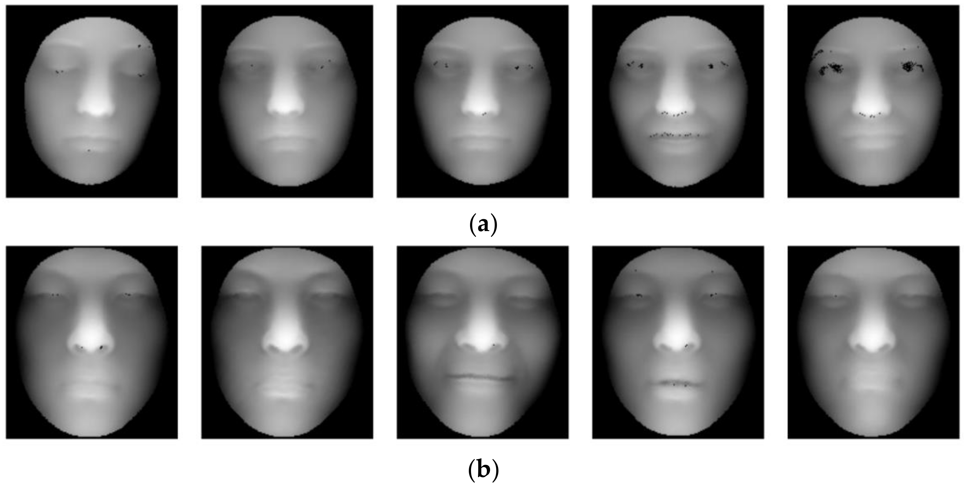
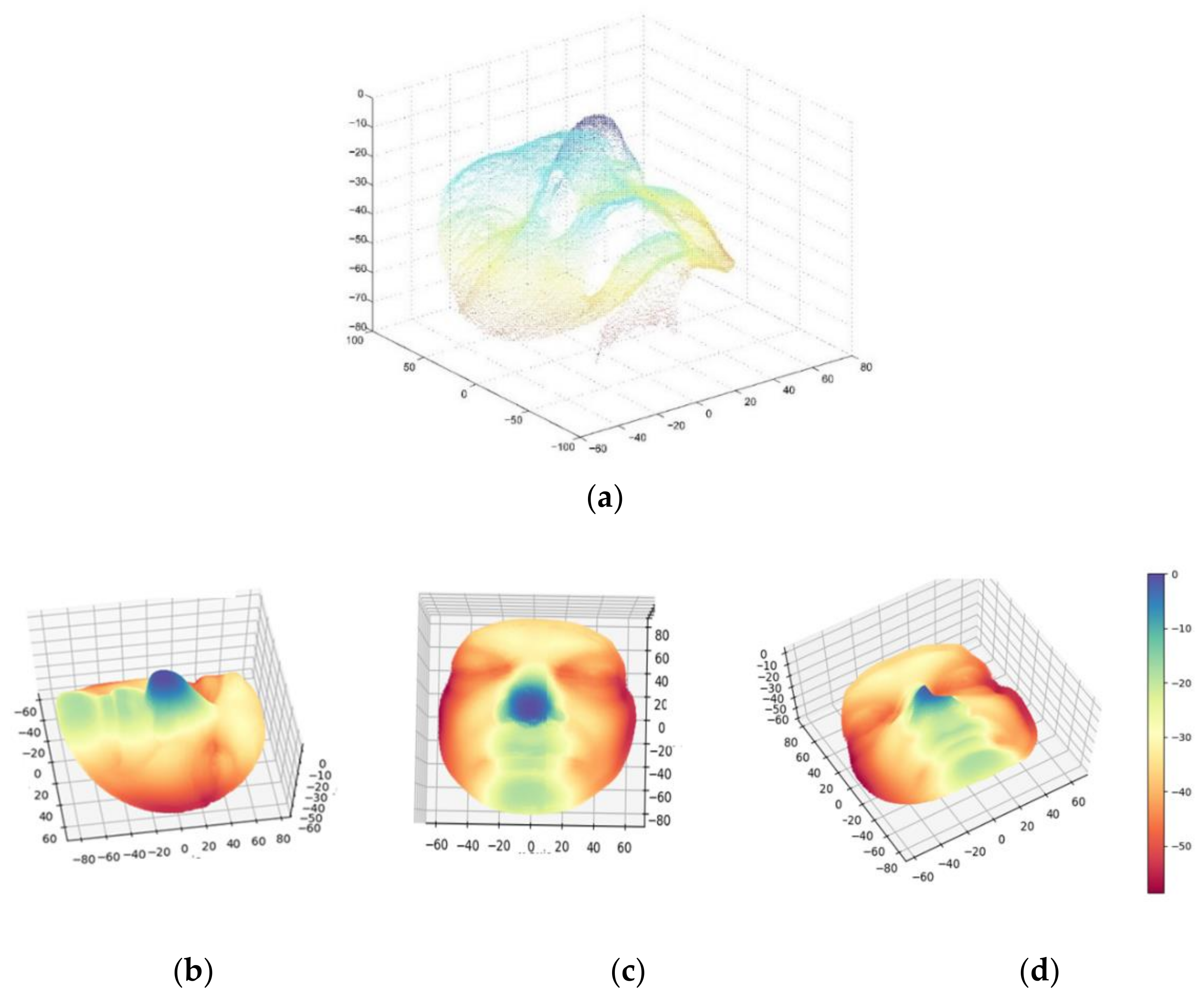
2.1. Dataset and Facial Scan Pre-Processing

The three-dimensional face data used in this study were obtained from the FRGC v2.0 Database [22], collected by the University of Notre Dame in the United States, and included 4007 frontal face scan images of 466 individuals. A total of 1–22 scanned images of each person were collected using a three-dimensional scanner in autumn 2003, spring 2004, and autumn 2004. The images included facial expressions, such as expressionless, smiling, laughing, frowning, bulging, surprised, and small changes in attitude. This database is currently one of the most widely used for face recognition.

Three-dimensional (3D) scanning data usually contain many redundant features including ears, hair, shoulders, and other areas unrelated to the human face, as well as outliers caused by the collection equipment and environmental conditions. Therefore, the face scan needs to be preprocessed. Firstly, outliers were eliminated; secondly, the shape index (SI) [23] could be used to identify the nose tip in order to correct the face position. The shape index was calculated as follow:

$$s=\frac{2}{\pi }\arctan \frac{{(\frac{\partial n}{\partial x})}_x+{(\frac{\partial n}{\partial x})}_y}{\sqrt{{({(\frac{\partial n}{\partial x})}_x-{(\frac{\partial n}{\partial y})}_y)}^2+4{(\frac{\partial n}{\partial x})}_y{(\frac{\partial n}{\partial y})}_x}}$$

(1)

where $s$ represents the shape index and ranges from −1 to 1; ${(\dots )}_x$ and ${(\dots )}_y$ represent the x component and y component of the vector in parentheses, respectively; $\frac{\partial n}{\partial x}$ and $\frac{\partial n}{\partial y}$ represents the vector formed by the corresponding point n in the x-direction and y-direction and the surrounding points, respectively. Different shape index values correspond to different curved surface shapes. The more concave curved surface has a smaller shape index, and the more prominent curved surface has a larger shape index. Finally, the face scan was interpolation smoothed. Figure 1 shows the visualization results of face point cloud data before and after pre-processing.

The pre-proposed point cloud image was projected and converted into a two-dimensional depth image, as shown in Figure 2. The face depth images were used to construct a small sample size dataset for face recognition in this work. More specifically, 995 face images were selected from 199 people with five different facial expressions in the FRGC spring 2004 data set. These face images were transformed into face depth images and classified into 199 classes according to people. Notably, in order to simulate the practical, small sample size situation, only five scans of each person were used as our experimental data, where 3 of each person were used for training, and the remaining 2 were used to estimate the performance of the proposed method.

2.2. Method

The process of the proposed face recognition algorithm is shown in Figure 3, and it includes three main phases: (1) Training phase: The pre-processed faces are used for transfer learning from the pre-trained ResNet18 weight to build a classification model. Then, the transferred weight is shared to construct a Siamese network that was fine-tuned for face binary classification with paired face samples. (2) Warehousing phase: The collected faces are transformed into a feature space. The features of the faces form a feature gallery for future face matching. (3) Testing phase: The input face is scanned and pre-processed to obtain a depth image. Then, the trained network will perform the forward operation to obtain the network output, which plays a role of confidence level to match faces.

2.2.1. Transfer Learning of Convolutional Neural Network Model for Face Recognition

We established a primary convolutional neural network, which can be used to extract facial features and achieve face classification when there are sufficient facial data and a small number of categories.

The convolutional layer in the network can be defined as:

$$S\left(i,j\right)=\left(I\times K\right)\left(i,j\right)=\sum _m\sum _{n}I\left(i-m,j-n\right)K\left(m,n\right)$$

(2)

where $I$ is the two-dimensional face scan input, $K$ is the two-dimensional kernel, $K\left(m,n\right)$ means the element $m,n$ of $K$, and $I\left(i-m,j-n\right)$ means element $i-m,j-n$ of $I$. The convolution neural network is able to map from different inputs to the same output and is thus widely applied for classification tasks. In our work, this characteristic is used to make our network expression-invariant.

Expression invariant means that for any input with different expressions from the same person, the network obtains the same output. Expression invariant can be defined as:

$$f\left({\mathit{x}}_{e_j}^{\left(i\right)};\mathit{\theta }\right)=f\left({\mathit{x}}_{e_k}^{\left(i\right)};\mathit{\theta }\right)$$

(3)

where $f\left({\mathit{x}}_{e_j}^{\left(i\right)};\mathit{\theta }\right)$ and $f\left({\mathit{x}}_{e_k}^{\left(i\right)};\mathit{\theta }\right)$ represent the output of the network with parameter $\mathit{\theta }$ when the input is ${\mathit{x}}_{e_j}^{\left(i\right)}$ and ${\mathit{x}}_{e_k}^{\left(i\right)}$, respectively. ${\mathit{x}}_{e_j}^{\left(i\right)}$ and ${\mathit{x}}_{e_k}^{\left(i\right)}$ means the 3D face scan from person $i$ with expression $e_j$ and $e_k$.

Some studies have shown that convolutional neural networks based on transfer learning have improved performance, which is mainly reflected in three aspects [24,25,26]. First, transfer learning may improve the initial network performance; second, transfer learning may increase the training speed of the network, making the performance improvement function of the network grow faster; finally, transfer learning may lead to better convergence, enabling the network to obtain a better training result.

In transfer learning, the learner must perform two or more different tasks, but we assume that many of the factors that explain the variations in P₁ are relevant to the variations that need to be captured for learning P₂. Many visual categories share low-level notions of edges and visual shapes, the effects of geometric changes, changes in lighting, and so on.

This characteristic of transfer learning can be observed in Figure 4, which shows the changes in network performance during the training process in two scenarios. The higher start point in Figure 4 indicates that the network using transfer learning has better initial performance, and the higher slope reflects the higher accuracy and speed of using transfer learning [27]. The final higher asymptote indicates that transfer learning has a more competitive final convergence effect.

When fewer face data are available, using transfer learning has a greater positive effect. Based on the excellent performance of transfer learning, transfer training of the face classifier was carried out in the form of transfer learning to construct a face feature extraction network.

At present, the more common convolutional neural networks include AlexNet [28], ResNet18 [29], and Vgg16 [30], among others. These neural networks have achieved good performance in related application fields. Choosing these neural networks for transfer learning can be more effective in improving the classification performance of the whole face recognition system. These three network structures have been proposed in different periods and have different network structures.

The output layers of these three networks all have a 1000-dimensional fully connected layer. The difference between the networks lies in the number of convolutional layers included and the network structure. In AlexNet and VGG16, the number configuration and sequential arrangement of convolutional layers differ. In ResNet18, the network contains a particular residual module represented as Conv-x. Through this module, the network can picture residual learning. We replaced the number of output dimensions of the original fully connected layer with the number of faces that need to be classified and performed transfer learning to form the required face classifier and construct a suitable convolutional network for the face feature extraction structure.

Considering that the network is a classification task in training, we used cross-entropy [31] as the loss function, which can be defined as follow:

$$J\left(\theta \right)=-{\mathbb{E}}_{x,y\sim {\widehat{p}}_{\mathrm{data}}}\log p_{\mathrm{model}}\left(y\mid x\right)$$

(4)

where $p_{\mathrm{model}}\left(y\mid x;\mathit{\theta }\right)$ means the output probability distribution of the model with parameter $\mathit{\theta }$ when the network input is $x$ and the ground truth output is $y$. $J\left(\mathit{\theta }\right)$ represents the loss function with the model parameter $\mathit{\theta }$. ${\widehat{p}}_{\mathrm{data}}$means the data empirical distribution. The cross-entropy function can measure the degree of difference between two different probability distributions in the same random variable. This was expressed as the difference between the true face label probability distribution and the predicted face label probability distribution. The smaller the value of cross-entropy, the better the prediction effect of the model.

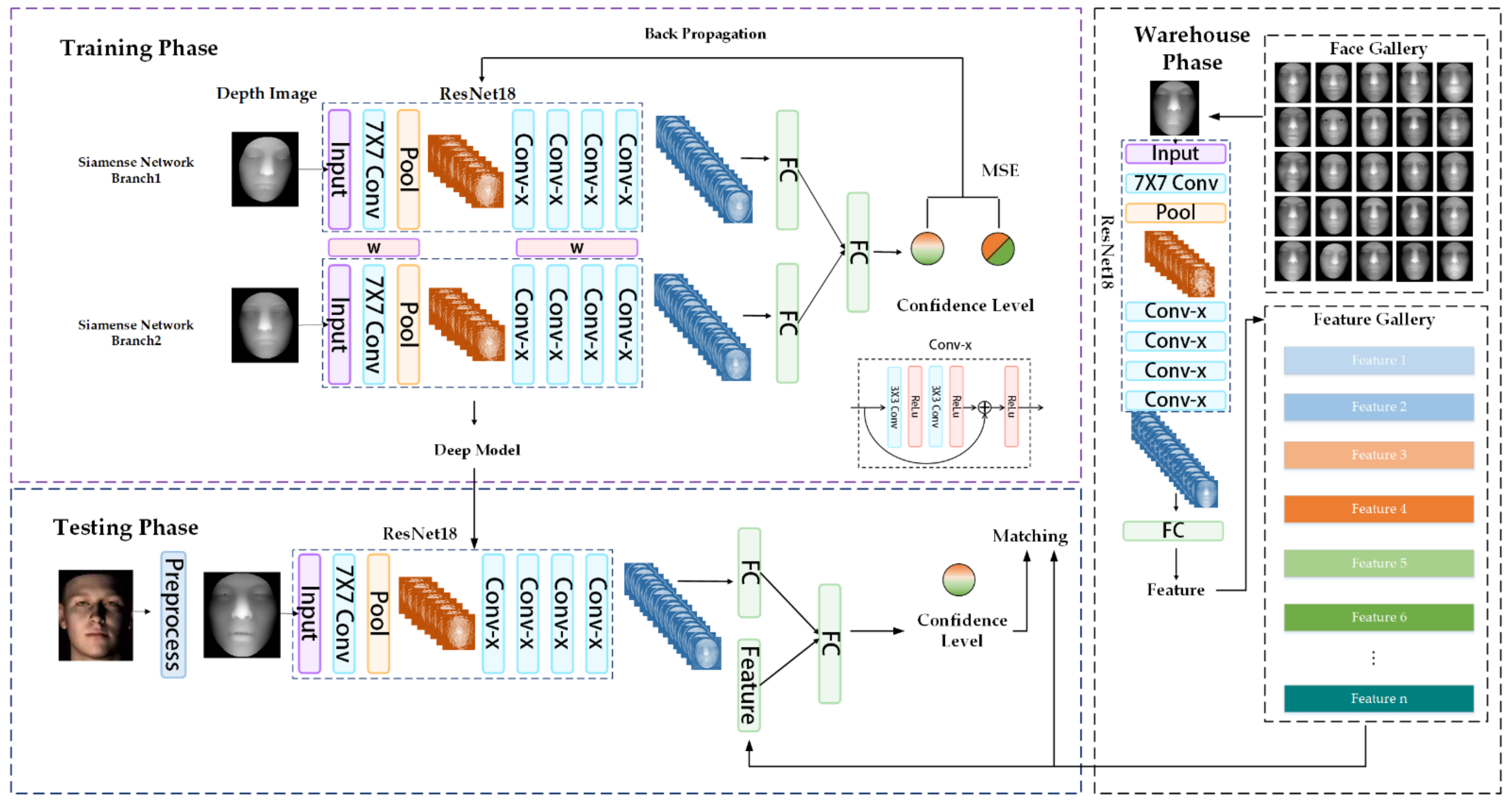
2.2.2. Siamese Network for Face Recognition

The convolutional neural network constructed could effectively extract the face area to achieve the classification task. However, as the number of categories increases, the accuracy of the classification decreases, and it is not possible to build an output layer for all people. Thus, we used a Siamese network to avoid this impact caused by the small number of samples.

There are two main differences between a Siamese network and a traditional convolutional neural network. In terms of neural network structure, the Siamese neural network constructs two convolutional neural network branches in the form of weight sharing, and the two branches are used to extract the prediction results from faces of two different persons or one person with two different expressions. In terms of the loss function, the Siamese neural network replaces the cross-entropy function commonly used in classification problems through a unique distance measurement method, which improves the network’s interpretability and makes the neural network feature extraction training more in line with the extraction difference of the gradient direction.

A transfer Siamese neural network can be constructed with the feature extraction results obtained by transfer learning, and its structure is shown in Figure 5. There are two feature extraction branches with shared weights. The w box in Figure 5 represents shared weights, which are used to extract facial features. A fully connected layer is used to complete the comprehensive mapping of features at the end of the network. Using the Siamese network, it is possible to transform the network mapping from a high-dimensional face image X to a low-dimensional encoding output. The detailed parameters of the network are listed in

Table 1. Architecture parameters of the proposed transfer Siamese network.

Layer Name	Output Size	Branch1	Branch2
Conv1	$112\times 112$	$7\times 7$, $64$, stride $2$	$7\times 7$, $64$, stride $2$
Conv2.x	$56\times 56$	$3\times 3$Max pooling, stride $2$	$3\times 3$ Max pooling, stride $2$
		$\left[\begin{array}{c}3\times 3, 64\\ 3\times 3, 64\end{array}\right]\times 2$	$\left[\begin{array}{c}3\times 3, 64\\ 3\times 3, 64\end{array}\right]\times 2$
Conv3.x	$28\times 28$	$\left[\begin{array}{c}3\times 3, 128\\ 3\times 3, 128\end{array}\right]\times 2$	$\left[\begin{array}{c}3\times 3, 128\\ 3\times 3, 128\end{array}\right]\times 2$
Conv4.x	$14\times 14$	$\left[\begin{array}{c}3\times 3, 256\\ 3\times 3, 256\end{array}\right]\times 2$	$\left[\begin{array}{c}3\times 3, 256\\ 3\times 3, 256\end{array}\right]\times 2$
Conv5.x	$7\times 7$	$\left[\begin{array}{c}3\times 3, 512\\ 3\times 3, 512\end{array}\right]\times 2$	$\left[\begin{array}{c}3\times 3, 512\\ 3\times 3, 512\end{array}\right]\times 2$
FC1	$500\times 1$	Average pool, 500-d fc	Average pool, 500-d fc
FC2	$1\times 1$	Average pool, 1-d fc

.

There are three more essential characteristics of the Siamese network. First, in the output code space, the distance in the code space can reflect the similarity of the input data in the high-dimensional space and the neighbor relationship. Second, the mapping is not limited by the distance of the input face data but can learn complex features inside the face data. Finally, this mapping can be effective for some new sample data with unknown neighbor relationships. Therefore, the face feature output layers are connected to a fully connected layer for the final regression, and the MSE loss function is adopted as the loss function to optimize the network.

3. Results and Discussion

To effectively evaluate the accuracy of face recognition with different numbers of categories, the classification accuracy of the face network for the test set was used as a unified evaluation index for the performance of different models, which was defined as follows:

$$ACC=\frac{N_c}{N},$$

(5)

where $N_c$ represents the number of correctly classified faces, $N$ represents the total number of faces, and $ACC$ represents the classification accuracy.

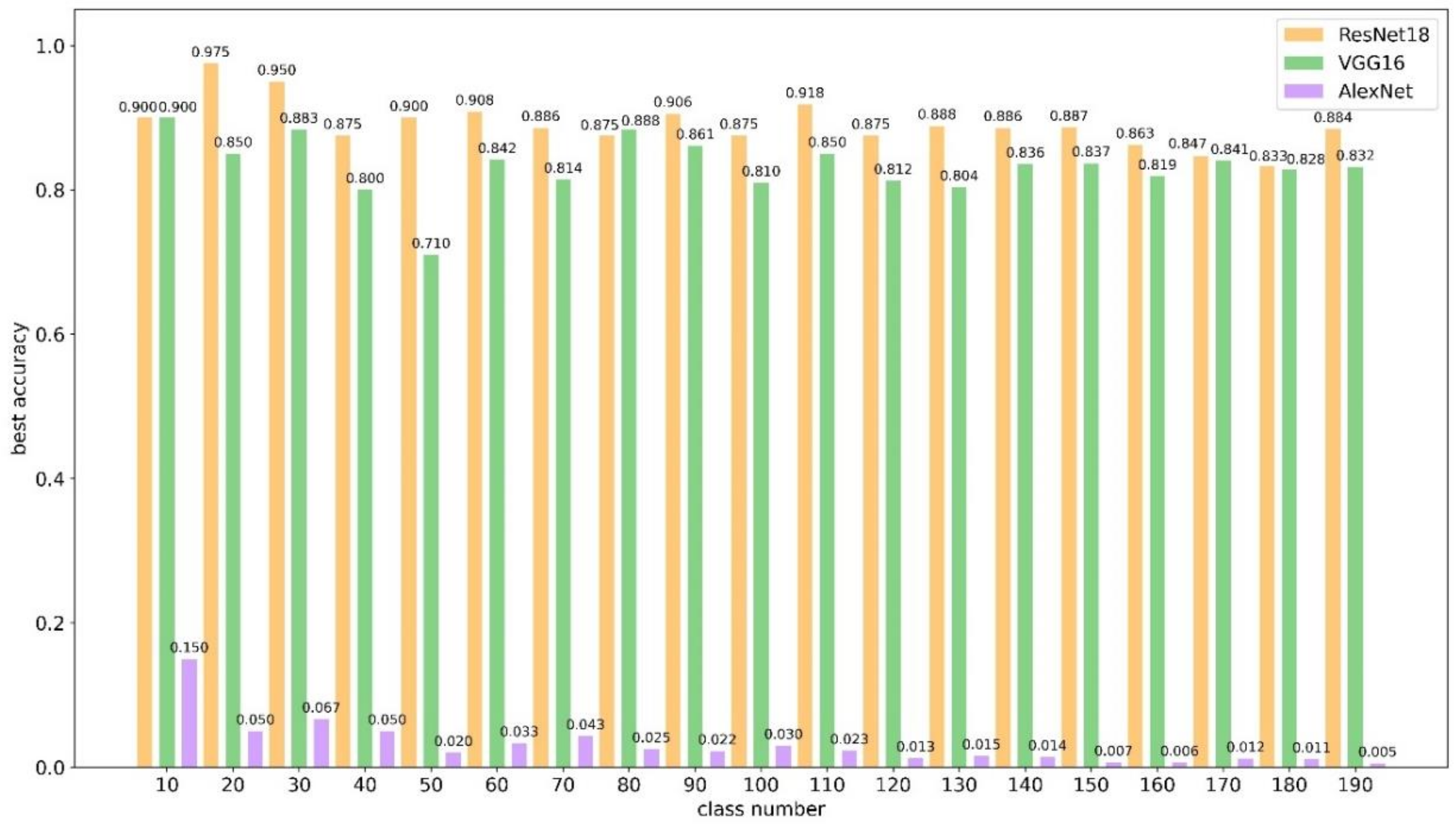
3.1. Evaluating the Effectiveness of Transfer Learning CNN

To compare the recognition effects of the three types of networks and the improvement in classification accuracy brought by transfer learning, the three convolutional network structures with different numbers of categories were trained separately, and the accuracy of the optimal results for each network after training was extracted. In the training process, the data used were the face data with at least five different expression images in the FRGC v2.0 database. We used a total of 199 groups of similar face data, and each experiment extracted the specified number of people from the 199 groups of face groups. Each group had five sample face data with different expressions, of which three were used for training, and the other two were used as validation data to simulate the practical, small sample condition. The highest accuracy of the validation data was used as the evaluation result for the model. The training algebra used was unified to 600 generations, the batch size for AlexNet was set to 128, and the batch size for VGG16 was set to 32 due to the limitation of the experimental hardware. From the training process of the experiment, we could observe the comparison of the training process with pre-training and without pre-training.

The accuracy and loss function decline performance of different types of training data during the training process has been improved which can be seen in Supplementary Material as Figures S1–S3. From the perspective of training accuracy, the use of transfer learning can increase the accuracy of the network more rapidly, and the final network convergence result was also more accurate. Transfer learning can make the loss function decline faster, and the result of convergence also has a lower loss value.

In addition, AlexNet had lower classification accuracy than the other two networks, and the convergence result of the loss function was also worse, as there was obvious over-fitting [32]. From Supplementary Material Figure S1b, it can be seen that the loss function of AlexNet first decreased and then increased. This is because the network was tested after over-fitting on the training set. There was a poor fit on the dataset, so the loss function increased after multiple generations. The same situation is evident in Supplementary Material Figure S3b, which is due to over-fitting of the training set. The ResNet18 network performed better than the VGG16 network, the final convergence result of the loss function was the lowest, and the prediction accuracy of the network was the highest.

In order to further evaluate the effectiveness of transfer learning, Figure 6 and Figure 7 show the face classifier’s classification results with different numbers of categories with and without transfer training. It can be seen from Figure 7 that without pre-training, the face classification accuracy of the AlexNet network was low, and it was almost impossible to classify faces effectively. This is because there was less training set algebra, and the amount of training data was small, so the convolution kernel in AlexNet could not be effectively trained, resulting in low classification accuracy. When the number of classification categories increased, the classification accuracy reduced further. When there were fewer classification categories, the experiment was more random, and the accuracy was not sufficient. Nevertheless, when there were fewer categories, the output end of the network was less challenging to map, which improved the classification accuracy.

The other two networks shown in Figure 7 had higher classification accuracy than AlexNet. Overall, the classification of ResNet18 was better than VGG16. This conclusion seems evident in Figure 7 after transfer training. This is because the residual module was included in the ResNet18 network structure, which can better extract the characteristics of the network through residual learning. Based on the above results, it can be seen that ResNet18 had the best performance in face classification tasks, followed by VGG16, while AlexNet had the poorest performance. The use of transfer learning improved the classification accuracy of all the networks, although this was particularly effective for AlexNet.

Table 2. Classification accuracy of models using different convolutional neural networks with and without transfer learning, where the data are in the format of $\mu \pm \mathsf{\Delta }x$, $\mu$ represents the mean value of the results, and $\mathsf{\Delta }x$ shows the confidence interval with a confidence limit of 0.95.

Number of Classes	With Transfer Learning			Without Transfer Learning
	ResNet18	VGG16	AlexNet	ResNet18	VGG16	AlexNet
10	94.2 ± 1.5	86.7 ± 1.9	91.7 ± 1.9	90.8 ± 1.5	91.7 ± 1.9	11.7 ± 1.9
20	89.2 ± 1.5	86.7 ± 0.9	75.8 ± 1.9	95.4 ± 1.8	83.3 ± 1.9	5.8 ± 1.5
30	95.5 ± 1.3	89.4 ± 1.8	80.0 ± 1.5	93.9 ± 1.3	88.3 ± 1.5	7.3 ± 1.8
40	98.0 ± 0.9	74.6 ± 1.4	74.2 ± 0.9	87.9 ± 1.4	80.4 ± 1.4	4.6 ± 1.8
50	92.0 ± 0.9	87.0 ± 0.9	72.7 ± 1.1	91.0 ± 1.2	70.3 ± 0.8	2.7 ± 0.8
60	97.3 ± 1.0	86.4 ± 1.0	66.1 ± 1.0	91.1 ± 0.9	84.2 ± 1.1	3.0 ± 0.9
70	96.4 ± 0.9	91.4 ± 0.6	65.7 ± 0.7	89.3 ± 0.6	82.1 ± 0.6	4.8 ± 0.9
80	96.0 ± 0.5	88.0 ± 0.2	72.1 ± 0.9	86.9 ± 0.5	88.8 ± 0.8	2.3 ± 0.7
90	94.3 ± 0.7	95.0 ± 0.7	71.8 ± 0.7	90.2 ± 0.7	86.3 ± 0.6	2.4 ± 0.6
100	94.8 ± 0.4	91.3 ± 0.5	74.8 ± 0.6	87.7 ± 0.5	81.2 ± 0.7	3.3 ± 0.6
110	96.2 ± 0.3	92.6 ± 0.5	68.3 ± 0.5	91.3 ± 0.4	84.8 ± 0.5	2.3 ± 0.4
120	94.3 ± 0.6	93.8 ± 0.4	68.0 ± 0.5	87.6 ± 0.2	81.5 ± 0.3	1.2 ± 0.6
130	97.3 ± 0.5	93.7 ± 0.4	71.2 ± 0.3	88.4 ± 0.5	80.8 ± 0.3	1.6 ± 0.6
140	94.7 ± 0.4	93.8 ± 0.4	64.2 ± 0.4	88.8 ± 0.4	83.8 ± 0.4	1.2 ± 0.4
150	95.9 ± 0.3	91.0 ± 0.4	71.1 ± 0.4	88.4 ± 0.4	83.6 ± 0.4	0.8 ± 0.2
160	95.4 ± 0.3	92.1 ± 0.4	67.4 ± 0.4	86.3 ± 0.3	82.2 ± 0.3	0.8 ± 0.2
170	96.0 ± 0.2	93.4 ± 0.3	66.7 ± 0.2	84.6 ± 0.3	84.2 ± 0.3	1.1 ± 0.3
180	94.5 ± 0.3	91.2 ± 0.2	64.7 ± 0.3	83.4 ± 0.3	83.0 ± 0.2	1.1 ± 0.3
190	96.0 ± 0.3	92.8 ± 0.2	63.2 ± 0.2	88.1 ± 0.2	83.1 ± 0.3	0.7 ± 0.2

shows the changes in classification accuracy of different models for classification with or without transfer learning. It is clear that the classification accuracy was improved when transfer learning was used. The average classification accuracy of ResNet18 after transfer learning was 95.2%, and the average classification accuracy without transfer learning was 89.0%, showing an increase of 6.2%. The average classification accuracy of VGG16 after transfer learning was 90.0%, and the average classification accuracy without transfer learning was 83.4%, showing an increase of 6.6%. The average classification accuracy of AlexNet after transfer learning was 71.0%, while the average classification accuracy without transfer learning was only 3.1%, showing an increase of 67.9%. These results indicate that transfer learning dramatically improved the accuracy of AlexNet’s face classification, and it also had a significant effect on the improvement of the classification accuracy of the other two networks. When there were fewer categories, the amount of test data was lower due to the small sample size. Therefore, when validation was performed, the validation accuracy was not sufficient to reflect the full performance of the network.

3.2. Evaluating the Effectiveness of Transfer Siamese Neural Network

To improve the coding stability of the network, a Siamese neural network was used to replace the traditional prediction structure. Using this structure can improve the network’s coding stability and make it less likely for over-fitting to occur.

Table 3. Classification accuracy of models using Siamese or not, where the convolutional network is ResNet18.

Number of Classes	Convolutional Network	Transfer Convolutional Network	Transfer Siamese Network
20	95.4 ± 1.8	89.2 ± 1.5	93.2 ± 1.8
50	91.0 ± 1.2	92.0 ± 0.9	94.6 ± 0.6
80	86.9 ± 0.5	96.0 ± 0.5	97.1 ± 0.5
110	91.3 ± 0.4	96.2 ± 0.3	97.3 ± 0.3
140	88.8 ± 0.4	94.7 ± 0.4	97.7 ± 0.1
170	84.6 ± 0.3	96.0 ± 0.2	97.6 ± 0.1
190	88.1 ± 0.2	96.0 ± 0.3	97.7 ± 0.1

shows the accuracy comparison of the transfer Siamese neural network and the convolutional transfer network for different numbers of face classes. For the convolutional network, the standard deviation of the classification accuracy was 0.0325; for the transfer convolutional network, it was 0.0251; and for the transfer Siamese neural network, it was 0.0166. The classification accuracy for the Siamese neural network was less sensitive to the number of classes. This is because the coding structure of the Siamese neural network has a fixed structure compared to the other networks and does not change with the number of samples. In addition, the accuracy comparison also shows that the face classification accuracy of the transfer Siamese neural network was higher than that of the other two networks.

3.3. Evaluating the Performance of Different Methods on Face Recognition

In order to test the validity of our algorithm, we conducted another experiment by calculating the overall accuracy of the proposed method. We conducted our algorithm five times and achieved the final average recognition rate shown in

Table 4. Classification accuracy of different models.

Method	Accuracy (%)
Mahoor et al. [33]	93.70
Tang et al. [7]	94.89
Lei et al. [6]	96.70
Deng et al. [34]	95.70
The proposed method	97.70

. The proposed method achieves the best 97.70% rank-one recognition performance on the FRGC v2.0 dataset. Comparing the rank-one recognition rate of several state-of-the-art results, the proposed method has slightly better performance than others. The improvement mainly relies on the robustness of the transferred convolutional layer and is further enhanced by the Siamese network architecture.

Computational efficiency is a critical concern for practical FR system application, which is one of the major advantages of the proposed method.

Table 5. Comparison of computation time (s) of the processing and matching.

Method	Processing	Matching	Total
Li et al. [35]	3.05	0.50	3.55
Lei et al. [36]	6.67	1.82	8.49
Kim et al. [4]	3.16	0.09	3.25
Cai et al. [9]	0.76	0.08	0.84
The proposed method	0.54	0.04	0.59

presents a timing comparison between the proposed method and several state-of-the-art methods that have published their computation times. The timing experiments were conducted on a PC with 3.2 GHz Intel Core processors and an NVIDIA GTX2080Ti GPU for training and testing using Pytorch implementation.

To analyze the computational cost of the proposed method, we recorded two computational costs, including processing time, which contains the time of processing and feature extracting, and matching time, which is consumed by feature matching. Our method spends less time in both processing and matching. The proposed method only extracts the feature based on one branch of the Siamese network from end to end in the testing phase, so the proposed method has an edge over the method in literature [9], which contains not only a network but also a manually designed feature augmentation. Moreover, the matching time is decreased by 2–45 times by replacing the classic Euclidean distance measurement with a simple two-layer fully connected network. The Euclidean distance measurement spends much time on L2 calculating, which is much more time-consuming than serval matrix product operation in a small neural network. Furthermore, the proposed approach can easily profit from parallel processing due to our neural network-based structure and the rapidly developing GPU-accelerated technique.

4. Conclusions

In this paper, we proposed a face recognition method based on a transfer learning convolutional network and Siamese network to solve small sample size issues and reduce the influence of facial expressions. In the face feature training phase, the pre-trained convolutional network was fine-tuned for expression-invariant face recognition. The experiment result shows that the transferred network significantly improved the performance of the network face recognition accuracy by 6.2% on average. The transferred network weights were utilized to construct a Siamese network. Random combinations of the samples were used as the dataset of the neural network for Siamese network training. Siamese neural network training made the network model more powerful in coding, which reduced the overall face data size from the raw 3D data and achieved a recognition accuracy of 97.7%.

In our future work, we will try to minimize the coding space of the proposed face feature generated network and the loss function of the proposed method may need to be changed to enhance the network distinguished part learning. The proposed method introduced a new kind of feature representation learning method with Siamese Network, which enriched the face-matching research field.

References

1. Zhang, X.; Gao, Y. Face recognition across pose: A review. Pattern Recognit. 2009, 42, 2876–2896. [Google Scholar] [CrossRef] [Green Version]
2. Wang, M.; Deng, W. Deep face recognition: A survey. Neurocomputing 2021, 429, 215–244. [Google Scholar] [CrossRef]
3. Manju, D.; Radha, V. A Novel Approach for Pose Invariant Face Recognition in Surveillance Videos. Procedia Comput. Sci. 2020, 167, 890–899. [Google Scholar] [CrossRef]
4. Kim, D.; Hernandez, M.; Choi, J.; Medioni, G. Deep 3D face identification. IEEE Int. Jt. Conf. Biom. 2018, 2018, 133–142. [Google Scholar] [CrossRef] [Green Version]
5. Adjabi, I.; Ouahabi, A.; Benzaoui, A.; Taleb-Ahmed, A. Past, present, and future of face recognition: A review. Electronics 2020, 9, 1188. [Google Scholar] [CrossRef]
6. Lei, Y.; Bennamoun, M.; Hayat, M.; Guo, Y. An efficient 3D face recognition approach using local geometrical signatures. Pattern Recognit. 2014, 47, 509–524. [Google Scholar] [CrossRef]
7. Tang, H.; Yin, B.; Sun, Y.; Hu, Y. 3D face recognition using local binary patterns. Signal Process. 2013, 93, 2190–2198. [Google Scholar] [CrossRef]
8. Cardia Neto, J.B.; Marana, A.N. Utilizing deep learning and 3DLBP for 3D Face recognition. In Iberoamerican Congress on Pattern Recognition; Springer: Berlin/Heidelberg, Germany; Volume 10657 LNCS, pp. 135–142. [CrossRef]
9. Cai, Y.; Lei, Y.; Yang, M.; You, Z.; Shan, S. A fast and robust 3D face recognition approach based on deeply learned face representation. Neurocomputing 2019, 363, 375–397. [Google Scholar] [CrossRef]
10. Liu, W.; Wen, Y.; Yu, Z.; Li, M.; Bhiksha, R.; Song, L. SphereFace: Deep Hypersphere Embedding for Face Recognition Weiyang. In Proceedings of the IEEE Conference on Computer Vision and Pattern Recognition, Honolulu, HI, USA, 21–26 July 2017; pp. 212–220. [Google Scholar]
11. Wang, H.; Wang, Y.; Zhou, Z.; Ji, X.; Gong, D.; Zhou, J. CosFace: Large Margin Cosine Loss for Deep Face Recognition Hao. In Proceedings of the IEEE Conference on Computer Vision and Pattern Recognition, Salt Lake City, UT, USA, 18–23 June 2018; pp. 5265–5274. [Google Scholar]
12. Deng, J.; Guo, J.; Xue, N.; Zafeiriou, S. ArcFace: Additive angular margin loss for deep face recognition. In Proceedings of the IEEE/CVF Conference on Computer Vision and Pattern Recognition, Long Beach, CA, USA, 15–20 June 2019; pp. 4685–4694. [Google Scholar] [CrossRef] [Green Version]
13. Meng, Q.; Zhao, S.; Huang, Z.; Zhou, F. MagFace: A Universal Representation for Face Recognition and Quality Assessment. In Proceedings of the IEEE/CVF Conference on Computer Vision and Pattern Recognition, Nashville, TE, USA, 21–24 June 2021; pp. 14225–14234. [Google Scholar]
14. Xiao, Y.; Li, J.; Du, B.; Wu, J.; Chang, J.; Zhang, W. MeMu: Metric correlation Siamese network and multi-class negative sampling for visual tracking. Pattern Recognit. 2020, 100, 107170. [Google Scholar] [CrossRef]
15. Kim, H.I.; Park, R.H. Siamese adversarial network for object tracking. Electron. Lett. 2019, 55, 88–90. [Google Scholar] [CrossRef]
16. Ahmed, N.K.; Hemayed, E.E.; Fayek, M.B. Hybrid siamese network for unconstrained face verification and clustering under limited resources. Big Data Cogn. Comput. 2020, 4, 19. [Google Scholar] [CrossRef]
17. Wang, G.; Wang, S.; Chi, W.; Liu, S.; Fan, D. A Person Reidentification Algorithm Based on Improved Siamese Network and Hard Sample. Math. Probl. Eng. 2020, 2020, 1–11. [Google Scholar] [CrossRef]
18. Sameer, V.U.; Naskar, R. Deep siamese network for limited labels classification in source camera identification. Multimed. Tools Appl. 2020, 79, 28079–28104. [Google Scholar] [CrossRef]
19. Figueroa-Mata, G.; Mata-Montero, E. Using a convolutional siamese network for image-based plant species identification with small datasets. Biomimetics 2020, 5, 8. [Google Scholar] [CrossRef] [PubMed] [Green Version]
20. Chang, S.; Li, W.; Zhang, Y.; Feng, Z. Online siamese network for visual object tracking. Sensors 2019, 19, 1858. [Google Scholar] [CrossRef] [PubMed] [Green Version]
21. Liu, F.; Zhao, Q.; Liu, X.; Zeng, D. Joint Face Alignment and 3D Face Reconstruction with Application to Face Recognition. IEEE Trans. Pattern Anal. Mach. Intell. 2020, 42, 664–678. [Google Scholar] [CrossRef] [PubMed] [Green Version]
22. Phillips, P.J.; Flynn, P.J.; Scruggs, T.; Bowyer, K.W.; Chang, J.; Hoffman, K.; Marques, J.; Min, J.; Worek, W. Overview of the face recognition grand challenge. In Proceedings of the 2005 IEEE Computer Society Conference on Computer Vision and Pattern Recognition, San Diego, CA, USA, 20–25 June 2005; Volume 1, pp. 947–954. [Google Scholar] [CrossRef]
23. Koenderink, J.J.; van Doorn, A.J. Surface shape and curvature scales. Image Vis. Comput. 1992, 10, 557–564. [Google Scholar] [CrossRef]
24. Zhuang, F.; Qi, Z.; Duan, K.; Xi, D.; Zhu, Y.; Zhu, H.; Xiong, H.; He, Q. A Comprehensive Survey on Transfer Learning. Proc. IEEE 2021, 109, 43–76. [Google Scholar] [CrossRef]
25. Lu, J.; Behbood, V.; Hao, P.; Zuo, H.; Xue, S.; Zhang, G. Transfer learning using computational intelligence: A survey. Knowl.-Based Syst. 2015, 80, 14–23. [Google Scholar] [CrossRef]
26. Weiss, K.; Khoshgoftaar, T. Evaluation of transfer learning algorithms using different base learners. In Proceedings of the 2017 IEEE 29th International Conference on Tools with Artificial Intelligence, Boston, MA, USA, 6–8 November 2017; pp. 187–196. [Google Scholar] [CrossRef]
27. Lisa, T.; Shavlik, J. Transfer learning. In Handbook of Research on Machine Learning Applications and Trends: Algorithms, Methods, and Techniques; IGI Global: Hershey, PA, USA, 2010; pp. 242–264. [Google Scholar]
28. Long, J.; Shelhamer, E.; Darrell, T. Fully convolutional networks for semantic segmentation. In Proceedings of the IEEE Computer Society Conference on Computer Vision and Pattern Recognition, Boston, MA, USA, 7–12 June 2015. [Google Scholar]
29. He, K.; Zhang, X.; Ren, S.; Sun, J. Deep residual learning for image recognition. In Proceedings of the 2016 IEEE Conference on Computer Vision and Pattern Recognition, Las Vegas, NV, USA, 27–30 June 2016; pp. 770–778. [Google Scholar] [CrossRef] [Green Version]
30. Urbonas, A.; Raudonis, V.; Maskeliunas, R.; Damaševičius, R. Automated identification of wood veneer surface defects using faster region-based convolutional neural network with data augmentation and transfer learning. Appl. Sci. 2019, 9, 4898. [Google Scholar] [CrossRef] [Green Version]
31. Goodfellow, I.; Bengio, Y.; Courville, A. Deep Learning; MIT Press: Cambridge, MA, USA, 2016. [Google Scholar]
32. Simon, H. Neural Networks and Learning Machines; Pearson Education India: London, UK, 2010. [Google Scholar]
33. Mahoor, M.H.; Abdel-Mottaleb, M. Face recognition based on 3D ridge images obtained from range data. Pattern Recognit. 2009, 42, 445–451. [Google Scholar] [CrossRef]
34. Deng, X.; Da, F.; Shao, H.; Jiang, Y. A multi-scale three-dimensional face recognition approach with sparse representation-based classifier and fusion of local covariance descriptors. Comput. Electr. Eng. 2020, 85, 106700. [Google Scholar] [CrossRef]
35. Li, H.; Huang, D.; Morvan, J.M.; Chen, L.; Wang, Y. Expression-robust 3D face recognition via weighted sparse representation of multi-scale and multi-component local normal patterns. Neurocomputing 2014, 133, 179–193. [Google Scholar] [CrossRef] [Green Version]
36. Lei, Y.; Guo, Y.; Hayat, M.; Bennamoun, M.; Zhou, X. A Two-Phase Weighted Collaborative Representation for 3D partial face recognition with single sample. Pattern Recognit. 2016, 52, 218–237. [Google Scholar] [CrossRef]
Figure 1. The pre-processed results of a 3D point cloud image, where (a) is the face scanned from the devices, and (bd) are the 3D face after removing outliers, interpolation operation, and smoothing from three angles. The values of the Z-axis in an image represent the distance between each point of the face and the tip of the nose, where red-colored dots are farther from the tip of the nose, and dots become more blue as the distance to the tip of the nose decreases.
Electronics 10 02128 g001
Figure 2. Transformed face depth images from 3D face data. (a) Six different expressions of Person A. (b) Six different expressions of Person B. The face expressions from the left to the right by column are expressionless, frowning, smiling, surprised, and small changes in attitude.
Electronics 10 02128 g002
Figure 3. Overview of the proposed 3D face recognition method.
Electronics 10 02128 g003
Figure 4. The effect of transfer learning on model performance.
Electronics 10 02128 g004
Figure 5. Structure of the transfer Siamese network.
Electronics 10 02128 g005
Figure 6. Accuracy of three different face classifiers without transfer training.
Electronics 10 02128 g006
Figure 7. Accuracy of three different face classifiers with transfer training.
Electronics 10 02128 g007