1. Introduction
Wireless Sensor Networks (WSNs) are composed of wireless sensor network nodes, which transmit the information collected in the detection area to the sink node in a self-organizing and multi-hop way, thereby actualizing the monitoring of the information in the detection area. With the development of the wireless network, WSN has been widely used in fine agriculture and smart factory and disaster prevention and reduction [
1]. In many types of research on wireless sensor networks, node deployment is one of the most fundamental problems because it is directly related to the network quality of service.
The earliest studies on the coverage of wireless sensor nodes mainly focused on the ideal two-dimensional plane [
2]. The nodes that adopted the two-dimensional disk-sensing model, the ant colony algorithm (ACO) [
3], and the cuckoo search algorithm (CS) [
4,
5] could improve the coverage of the target area in the two-dimensional plane. A 3D spherical sensing model based on 3D space coverage was proposed to study the coverage problem further [
6]. Mnasri [
7] compared 2D deployment with 3D deployment and proved that the latter was more complex because it could solve more constraints brought by practical problems. Boufares [
8] proposed a distributed algorithm based on virtual force to actualize autonomous coverage of the sensor nodes in the 3D region. Du [
9] combined distributed particle swarm optimization (DPSO) algorithm with the virtual force algorithm (VF) and demonstrated the superiority of this algorithm in solving the performance of deployment nodes in the 3D environment. Furthermore, in order to better account for the signal attenuation problem in practice, the probabilistic perception model based on disk and sphere has been gradually used to solve the deployment problem of WSN nodes [
10]. Hossain [
11] discussed the influence of different sensor coverage models on the network coverage range. Hao [
12] proposed a 3D coverage deployment method based on WSN probabilistic model and proved the effectiveness of the method.
The three-dimensional surface-coverage problem is a particular type of problem in WSN node deployment [
13]. The WSN nodes are distributed on a three-dimensional surface to complete the task of covering the surface. The WSN coverage problem in 3D terrain is close to actuality and has a certain degree of complexity, so there are few related studies [
14,
15,
16,
17]. The general solution to the covering problem of the complex surface is as follows:
The functional surface is used to simulate the surface environment of the area to be deployed.
The three-dimensional spherical covering model is adopted as the covering model of WSN nodes.
Use heuristic optimization algorithms (such as PSO, GA, ACO, etc.) to complete nodes’ deployment.
The current states and progress of the 3D surface-covering problem are outlined: Boufares [
18] proposes a distributed deployment algorithm (3D-IDVFA-TC) based on the improved virtual force strategy, which can effectively improve the coverage rate of different complex Z-degree surface function models while ensuring network connectivity and reducing node loss. Saha and Saikia [
19] proposed a method based on Delaunay triangulation and projection to optimize sensor node deployment in hilly areas. Felamban [
20] obtained the deployment location of nodes through the three-dimensional filling of the truncated octahedron.
Although the above algorithms can achieve a better deployment effect in the WSN surface-coverage problem, four significant issues have yet to be addressed: first of all, the model of the area to be deployed still uses the simple surface generated by the function, which is too regular and smooth to simulate the surface characteristics of the real terrain environment. Secondly, the above solution needs to estimate the required number of nodes based on the surface function. However, due to the irregularity of the real terrain, it cannot obtain the surface function of the area and consequently cannot calculate the number of nodes. Thirdly, the coverage of nodes is primarily irregular shapes in the complex surface environment, but the traditional spherical coverage model does not consider the impact of the real terrain on coverage. Therefore, it is urgent to propose a node coverage model that fits the real surface environment better. Finally, the previous deployment algorithms are easy to fall into local optimum and slow convergence because of the large amount of surface information data in the monitoring area, and the new coverage model is more complex. Therefore, to solve the WSN deployment problem of real three-dimensional terrain more effectively, a deployment algorithm that can fully integrate terrain data and node coverage model characteristics is required.
Based on the above ideas, this paper proposes a WSN node deployment algorithm based on real three-dimensional terrain, which uses the real terrain elevation data downloaded from a network geographic database to reconstruct and model the surface. A probabilistic coverage model based on Digital Elevation Model (DEM) data is proposed, which can more truly reflect the influence of the geographical environment on the coverage of nodes. Finally, considering the efficiency of the Greedy algorithm in solving the optimal solution problem, we combine the Greedy algorithm for node deployment. Simulation results verify that the proposed coverage model can reflect the real coverage more realistically under diverse surface models with different complexity. Meanwhile, combined with the idea of the Greedy algorithm, it can quickly complete the deployment of nodes and achieve a higher coverage rate.
The contributions of this study are as follows:
Terrain-modeling technology based on DEM data is applied to solve the WSN node deployment problem, which actualizes the visualization of the WSN node’s three-dimensional surface deployment plan.
A WSN probabilistic coverage model based on DEM data is proposed in this study. This model considers factors such as signal attenuation and terrain occlusion on the original basis, making the coverage model closer to actuality and more practical.
The Greedy algorithm based on grid scanning is employed to solve the WSN node coverage problem, which significantly reduced the time and space complexity of the algorithm.
The remainder is assigned as follows.
Section 2 introduces the methods and steps of establishing a three-dimensional real surface model. In
Section 3, the proposed probabilistic coverage model of WSN based on DEM data is described in detail. In
Section 4, an efficient sensor deployment algorithm on 3D real terrain is presented.
Section 5 conducted a series of simulation comparison tests. Finally, a conclusion is provided in
Section 6.
2. Real Three-Dimensional Surface Model
In this section, we will introduce the methods of constructing the real three-dimensional surface models, including the acquisition and processing of DEM data and commonly used modeling methods and comparisons. Constructing a real three-dimensional surface model can reflect the real terrain characteristics of the area to be deployed and provide a reference for subsequent node deployment decisions.
The geographic data used in this study comes from the Geospatial Data Cloud [
21]. It provides a large amount of real surface data information for downloading, and the data types are rich and diverse. Among them, the Digital Elevation Model, or DEM for short, actualizes the digital simulation of the ground terrain through limited terrain elevation data (that is, the digital expression of the terrain surface morphology). It is a solid-ground model that uses a set of ordered numerical arrays to represent ground elevation. The DEM file in the image format was opened by Global Mapper, then the image was intercepted and ultimately converted into evaluation value data output.
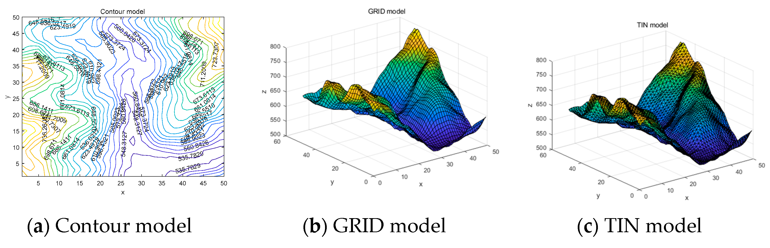
Commonly used DEM data representation models are the contour model, regular grid model (GRID), and irregular triangular network model (TIN), as shown in
Figure 1. The contour model emphasizes the topography features through contour lines, shows the steepness of the slope through the density between the lines, and can directly display the height of the terrain with elevation data. However, it cannot visually display the overall topography and geomorphology. Although the GRID model and the TIN model cannot display topographical changes in the form of data, they can intuitively reflect the general appearance of the terrain and have a higher degree of visualization.
Both the GRID model and the TIN model have the advantages of fully expressing the structural features of the terrain. However, compared with the TIN model, the GRID model has a more straightforward structure, a smaller amount of stored data, and is more convenient for analyzing and calculating the terrain later. Therefore, we choose the GRID model to establish the surface model.
The general modeling steps of the GRID model are: first, mesh the plane area according to the number of samples of the DEM points in the horizontal and vertical directions, and then, assign the corresponding elevation values to the grid points.
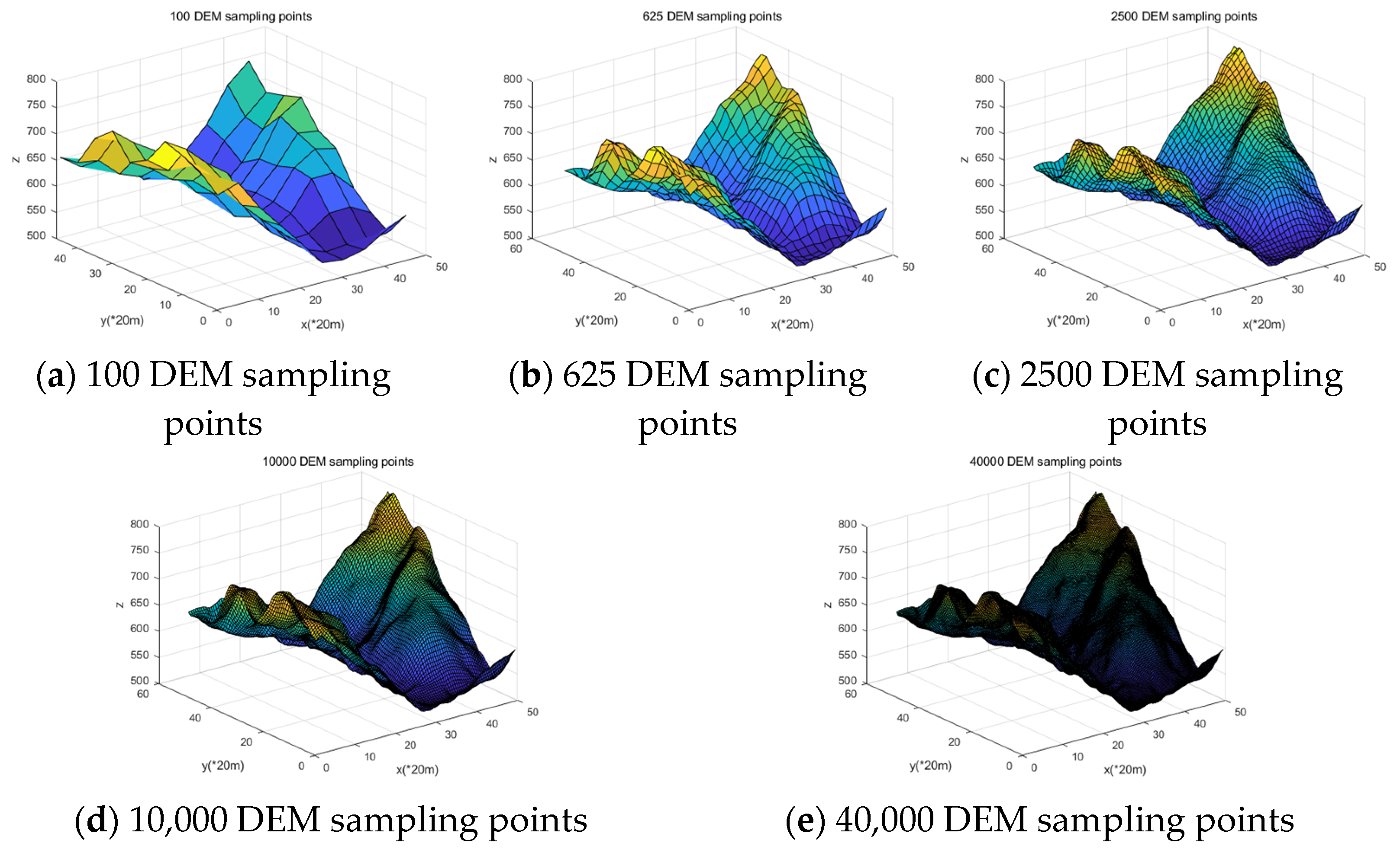
The amount of DEM data used to construct the surface model is closely related to the modeling accuracy. As shown in
Figure 2, the higher the DEM data volume, the higher the sampling accuracy. It means the larger the data storage and the more complicated the calculation. Selecting appropriate modeling accuracy can reduce the number of model calculations and save time and cost while meeting the coverage requirements.
3. Probabilistic Coverage Model of WSN Based on DEM Data
3.1. Problem Formulation
For the problem of WSN on surface coverage, the most commonly used node coverage model is spherical, and the coverage criterion is a single distance criterion that can only be declared to be covered if the spatial distance is smaller than the node coverage radius. In the following Formula (1):
where
P is the coverage probability,
d is the distance from the node, and
r is the node coverage radius.
In practical applications, the deployment environment of WSN nodes is primarily mountainous terrain with large undulations and irregularities, where the coverage of nodes is easily affected by the terrain. In this case, using the traditional spherical coverage model will cause an error between the real coverage and the calculated results. Suppose that the node is deployed at position 1 using the traditional spherical coverage model. In this case, point 2 can be covered in
Figure 3, but the actual situation is that the terrain occludes the coverage blind area, and electromagnetic waves cannot cover the two points.
In order to solve the above problem, a WSN probability coverage model based on DEM data is proposed. Based on the traditional coverage model, it considers the influence of signal attenuation and terrain occlusion factors on the coverage model, which agrees well with the perceived characteristics of nodes in practical applications.
3.2. Coverage Model Construction
3.2.1. The Influence of Terrain-Shading Factors on the Coverage Model
Since the continuous terrain surface is discretized into DEM data points (x, y, z), then the continuous surface-coverage problem is transformed into a discrete grid point coverage problem. Now we will proceed with the following steps to solve this problem.
First, store the coordinates
of all discrete grid points on the three-dimensional surface model into the matrixes
X,
Y,
Z, respectively shown in Equation (2), where the coordinate
is the elevation coordinate value corresponding to the grid point
:
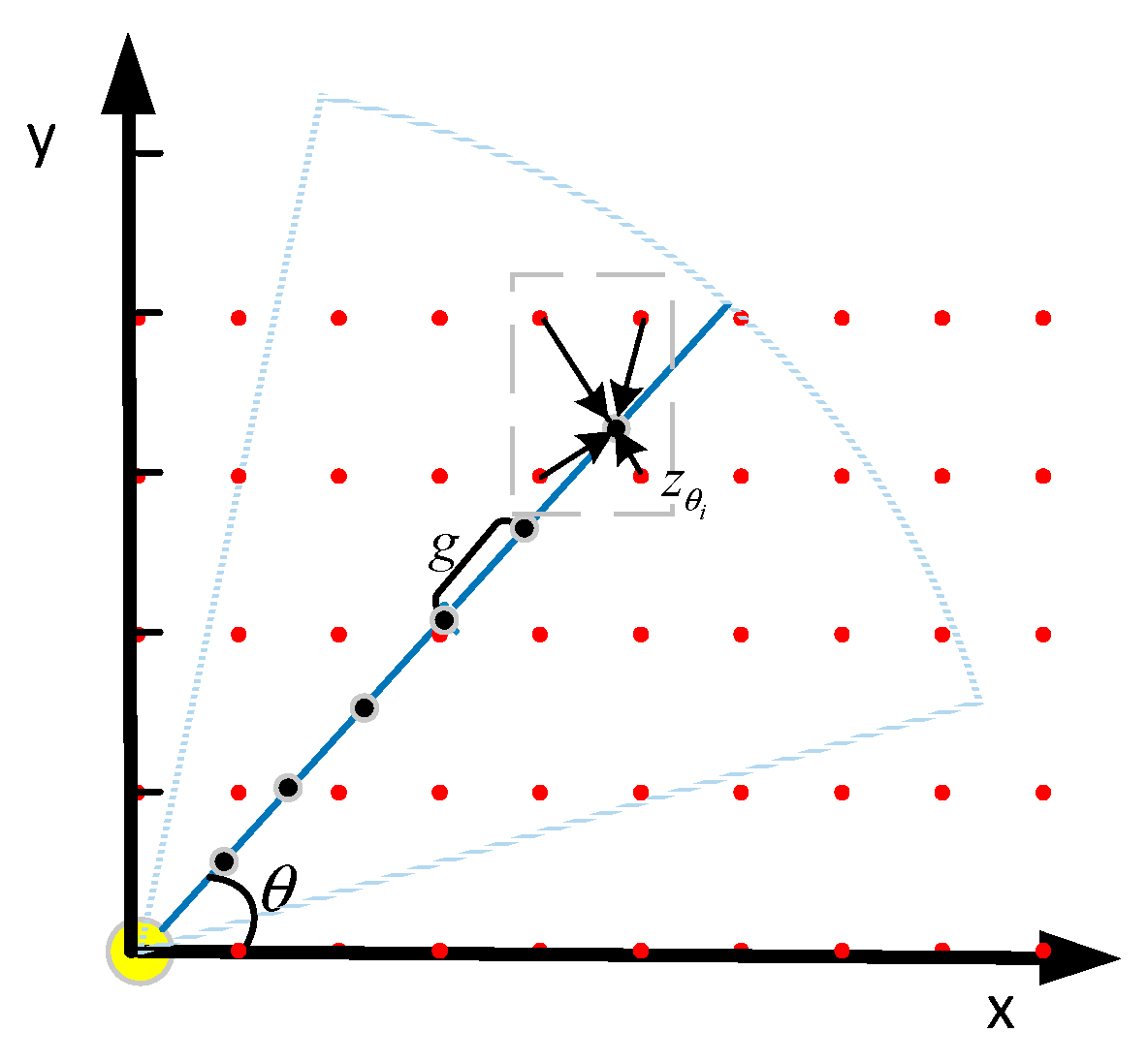
For determining the influence of the terrain occlusion in any sensing direction of the sensor node, it is necessary to estimate the ground surface height in this direction since the terrain surface is discretized into elevation points, as shown in
Figure 4. For any sensor node with a sensing radius of
r on a discrete grid point, taking the node coordinates as the origin, the sensing direction angle
as the step direction, and
g/cos
θ as the step length, where
g is the distance between discrete grid points. The elevation value of each stepped point is calculated by interpolation of the four surrounding grid points. Then, the elevation values
for all step points within the perceptual range
r in the perceptual direction
θ can be obtained.
Based on the approximate elevation values
, Equation (3) determines how the grid points in the sensing direction are affected by the terrain shading.
means that sensor node can cover the grid points without being affected by the terrain, and
implies that the grid points cannot be covered by the influence of terrain occlusion.
is the elevation value of the corresponding step point of the sensor node in the sensing direction,
z0 is the elevation value of the grid point where the sensor node is located, and
zn is the farthest grid point that the sensor node can perceive in the sensing direction:
An illustrative example is shown in
Figure 5; it can be calculated that the grid points
in the figure are affected by the terrain shading. According to Equation (3), grid points 2, 4, and 6 are affected by the grid points located in front of them and have larger elevation values, which block the sensory signal of the node, resulting in coverage blind spots, as shown in
Table 1.
By increasing the sensing direction angle θ in the range , it can be determined whether each grid point in the sensing range of the node is affected by the terrain occlusion.
3.2.2. The Influence of Signal-Attenuation Factors on Coverage Model
Furthermore, to account for the influence of signal propagation attenuation on the coverage model, we combine the terrain shading influence criterion with the spherical probability perception model [
7].
The coverage probability of the spherical probability perception model changes with the distance of the node. Mathematically, the coverage probability is shown in Equation (4). This model avoids the traditional Boolean perception model’s cliff-like perception boundary and is closer to the actual propagation of the perception signal:
where
Psph is the probability that can perceive a specific grid point under the spherical probability coverage model,
d denotes the distance between the grid point and the node,
R represents the maximum sensing radius when there is no signal attenuation, and
r is used to describe the uncertainty perception ability of the node,
.
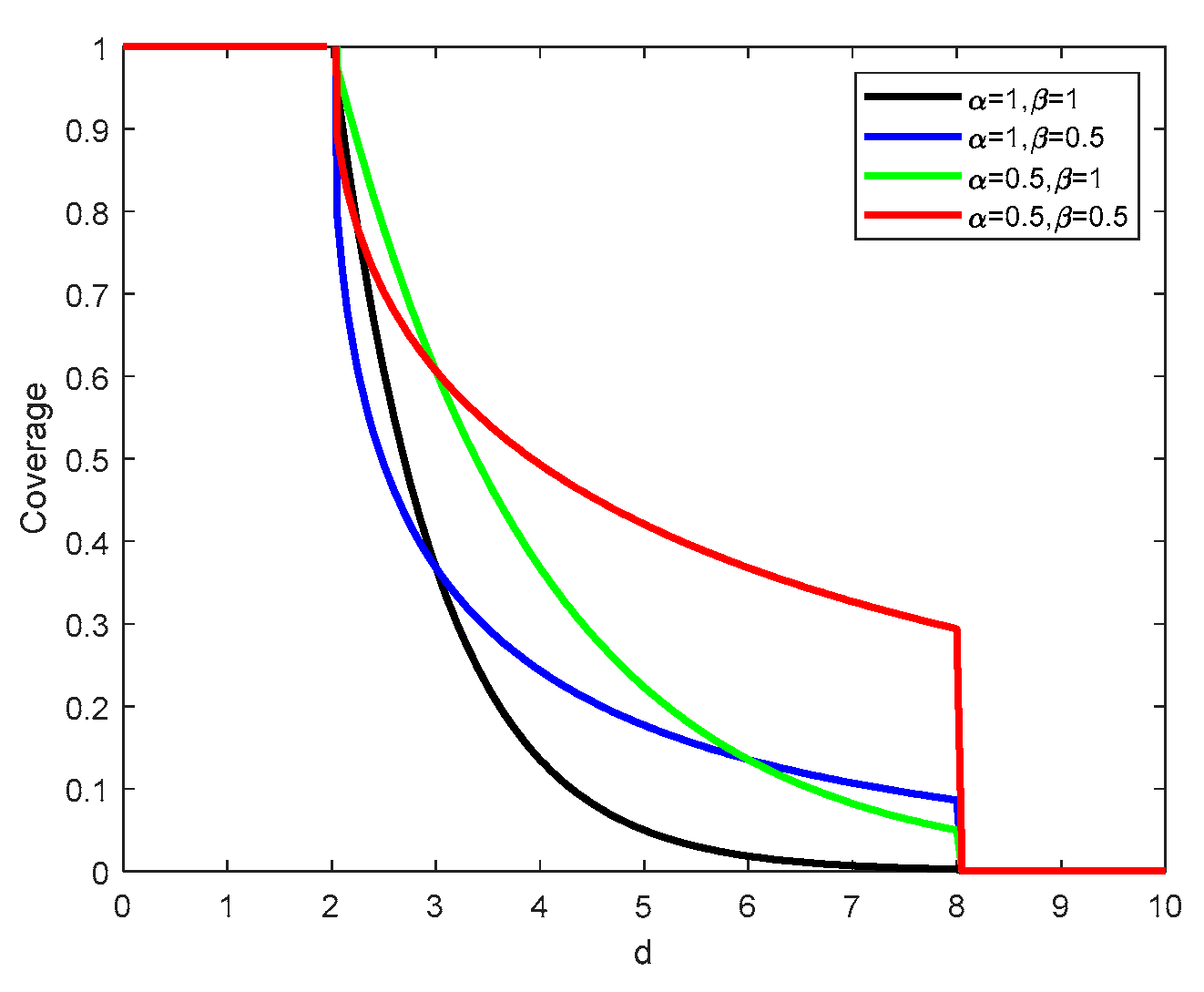
are attenuation factors that determine the degree of attenuation of the perceived probability of a node in an uncertain sensing region with distance. The relationship between
and
is shown in
Figure 6. In the figure,
R is set to 5 and
r is 3. When
, the perceived probability decays faster. When
, the probability decays slowly. The values of
can be selected according to the actual situation of the node to meet different coverage requirements.
3.2.3. The Influence of Signal Attenuation Factors on the Coverage Model
Finally, combining the above two models, the WSN probability attenuation coverage model based on DEM data is obtained as:
This model comprehensively considers the influence of the terrain shading and signal attenuation on the node coverage model, so the model can more genuinely reflect the perceived effect of the node in the actual environment.
4. WSN Deployment Based on Grid Scanning Using the Greedy Algorithm
The Greedy algorithm is a typical heuristic algorithm. It makes the current best choice at every step, which means that it is not considering optimization as a whole, but a local optimization. However, this kind of optimal local solution is often relatively close to the optimal global solution. Greedy algorithms tend to save more time and cost than global optimization algorithms to solve problems.
A solution for the deployment of WSN nodes on real 3D terrain is proposed. The probabilistic attenuation coverage model of DEM data is adopted for nodes, and the Greedy idea is used for node deployment on the real three-dimensional surface model. Its basic idea is as follows:
First of all, the problem to be solved needs to be clarified. The solution goal of this study is to actualize the deployment of sensor nodes under the complex and three-dimensional surface model and maximize the coverage rate while meeting the regional coverage requirements. Therefore, the objective function is:
where
is the coverage rate under the condition that the preset coverage rate
is satisfied, and its calculation formula is the ratio of the number of covered grids to the total number of grids, where the coverage is declared when the probability
is greater than a specified threshold
.
Then, the constraint conditions of the algorithm are determined: the deployment position of the candidate nodes cannot exceed the deployment range defined by the area to be deployed. That is, all nodes are deployed on the grid points divided by the surface model. Suppose the sensor coordinate of a node is
, and the corresponding constraint condition is:
Node traversal is carried out according to the idea of the grid-scanning Greedy algorithm.
- (1)
Calculate the coverage P(k) of any sensor node to its surrounding grid points under the influence of terrain shading and signal attenuation by combining Equations (3)–(5).
- (2)
Find the node deployment location that can cover the largest number of grid points in the area to be deployed, and add this location to the candidate coverage set
, as shown in Equation (8):
- (3)
Delete the covered grid points from the traversal domain
Trav. Suppose multiple nodes with the same coverage rate are encountered during the traversal process. In that case, the node with the smallest coordinate is selected for priority deployment until the area to be deployed is fully covered or the predetermined coverage rate is reached, and finally ends the algorithm. The specific formula is shown below:
The implementation of the WSN node deployment algorithm based on real 3D terrain is summarized in Algorithm 1:
| Algorithm 1: WSN deployment based on grid scanning using the Greedy algorithm |
| 1 Import of DEM Data. |
| 2 Initialize . |
| 3 For each surface grid . |
| 4 Calculate the coverage area corresponding to the grid point . (3)–(5) |
| 5 End. |
| 6 While () |
| 7 Find the location of the node to be deployed with the largest coverage. (8) |
| 8 Add the point to the candidate coverage set. (8)
|
| 9 Remove the covered grid points from the traversal domain. (9) |
| 10 IF |
| 11 IF |
|
12 ; |
| 13 Else |
| 14 ; |
| 15 End. |
5. Simulation Experiments and Analysis
To verify the superiority of the proposed algorithm (GAGS) in solving the 3D complex-surface-coverage problem, we will compare and simulate it with traditional deployment algorithms (PSO, GA, ACO).
First, the coverage of each algorithm is compared through deployment simulations under three surface models of different complexity. Secondly, the coverage attenuation factor, coverage threshold, and preset coverage values in the coverage model were changed and simulated again to test the coverage performance of each algorithm under the coverage model of different parameters. Finally, the iterative time required for different algorithms to complete the deployment plan is compared.
5.1. Deployment Simulation under Different Levels of the Complex Surface Model
Deployment simulations on three surface models with different levels of complexity are performed, and the coverage rate that each algorithm can achieve is compared. The deployment parameters of all algorithms are kept consistent, as shown in
Table 2.
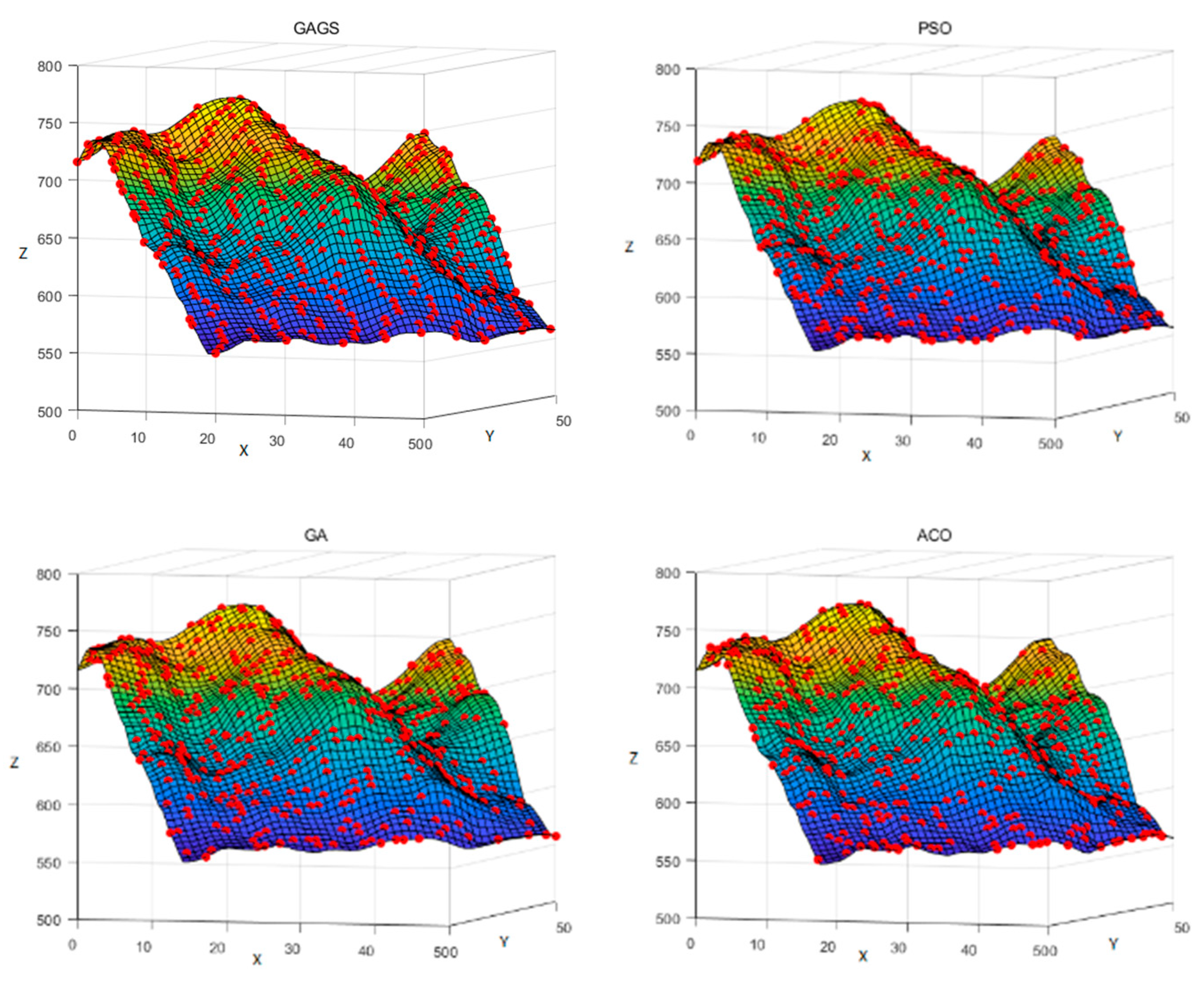
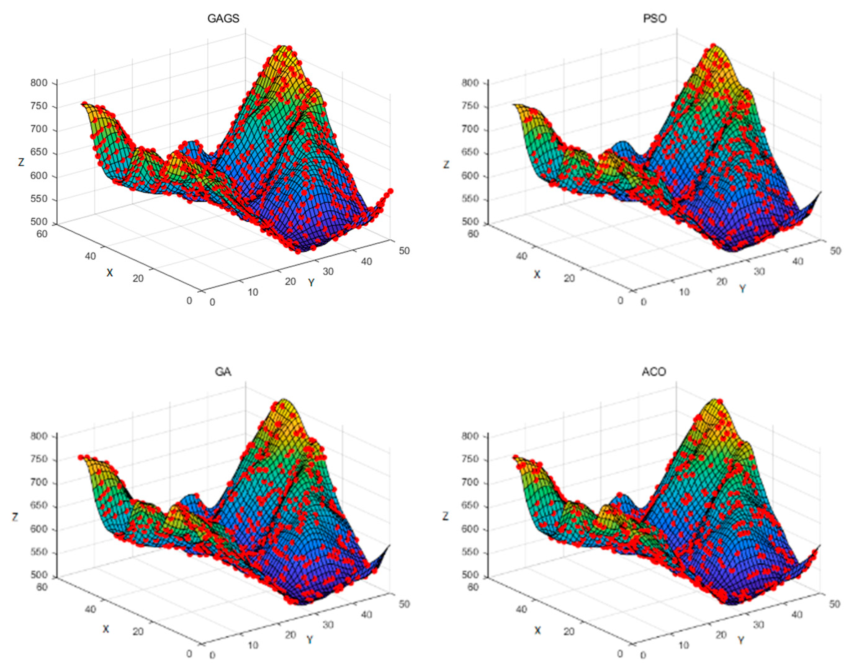
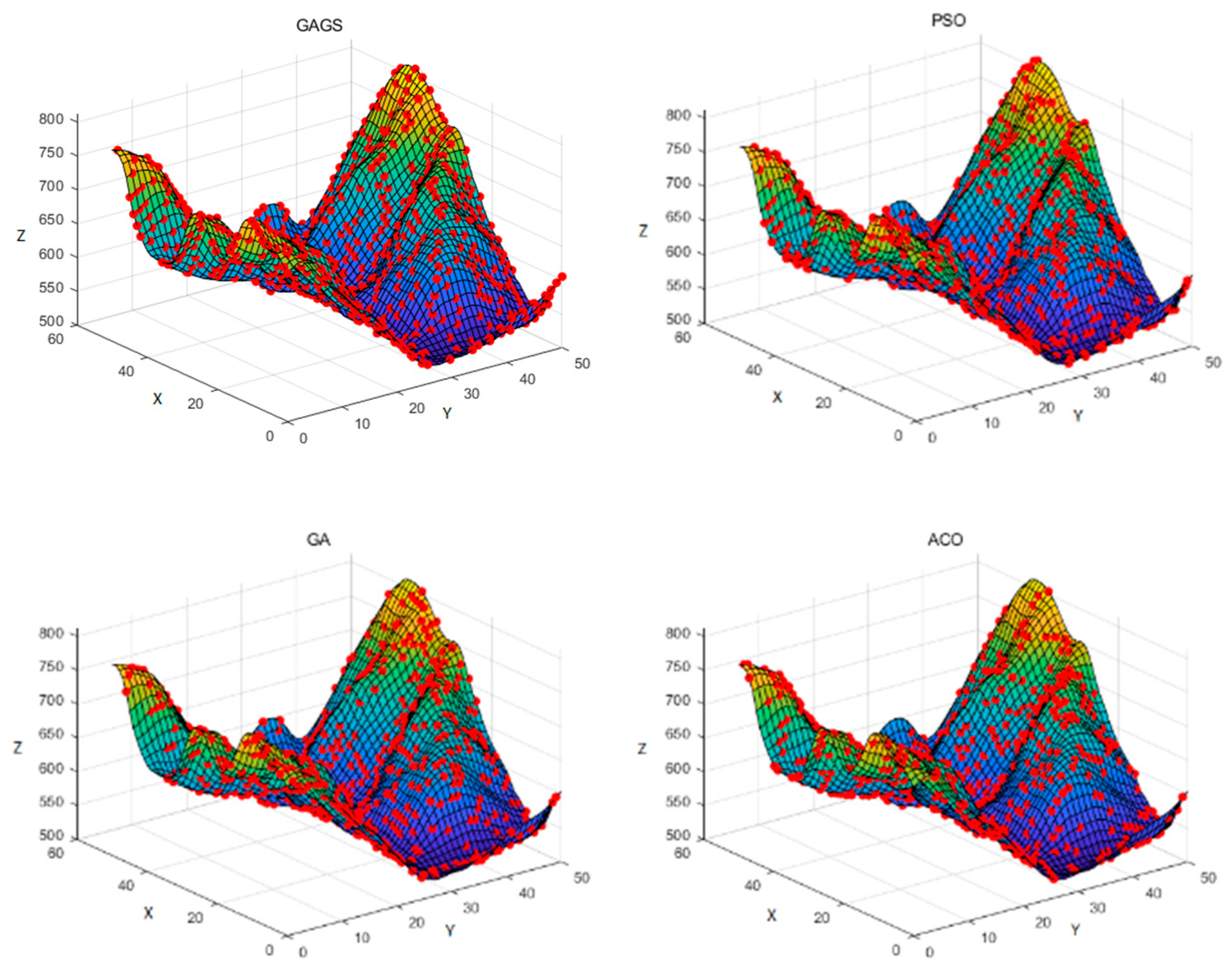
The deployment results are shown in
Figure 7,
Figure 8 and
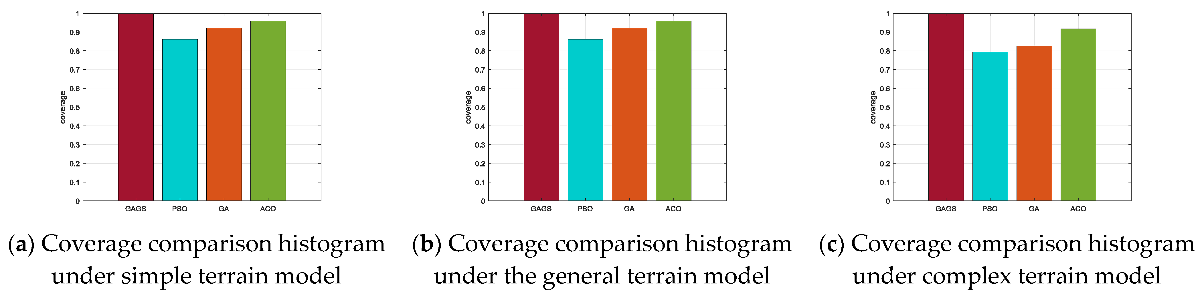
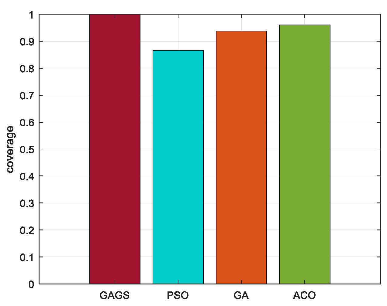
Figure 9. The deployment results of the proposed GAGS are more uniform than the other algorithms. Furthermore, to more intuitively demonstrate the superiority of the proposed algorithm in terms of coverage, we compare the coverage rate of different algorithms after deployment, as shown in
Figure 10.
Specifically, when deploying nodes using a simple surface model, as shown in
Figure 7, GAGS uses 444 nodes to achieve full coverage. When the same number of nodes are deployed, the deployment coverage rate of PSO is 86.12% and GA and ACO were 92.04%, 95.99%, respectively, as shown in
Figure 10a.
Figure 8 presents the deployment simulation of nodes using the general surface model. Since the surface model’s projected area is the same, increasing the terrain complexity will increase the surface area and correspond to the number of nodes that need to be deployed. In this case, GAGS uses 486 nodes to achieve full coverage, but when the number of deployed nodes is the same, the deployment coverage of PSO is 83.24%, and GA and ACO are 83.52% and 93.56%, respectively, as is shown in
Figure 10b.
Using a complex surface model (
Figure 9), GAGS uses 630 nodes to achieve full coverage. In the same number of deployed nodes, the deployment coverage of PSO is 79.33% and GA and ACO are 82.67% and 91.69%, respectively. Compared with the simple terrain model, the coverage descent further, as shown in
Figure 10c.
5.2. Deployment Simulation under Different Coverage Model Parameters
Take the complex surface model in
Figure 9 as an example. The coverage of GAGS under the coverage model with different parameters of the attenuation factor
α,
β, the threshold
φ, and the value of the preset coverage are analyzed individually.
5.2.1. Deployment Simulation with Different Attenuation Factors
While keeping the other simulation parameters unchanged, the coverage model attenuation factors
α,
β were increased from 0.5 to 1. The deployment results of each algorithm are shown in
Figure 11.
Since the increase of the attenuation factors
α,
β will accelerate the attenuation speed of the coverage rate of the perception model, the effective coverage area of each node will be relatively reduced, leading to an increase in the number of WSN nodes to achieve full coverage of the area. The deployment coverage of each algorithm can be seen in
Figure 12.
After increasing the attenuation factors α, β, GAGS achieves full coverage with 684 WSN nodes, while when deploying the same number of nodes, the coverage rate of PSO is only 86.6%, the coverage rate of GA is 93.79%, and that of ACO reached 96.04%. It reveals that the GAGS algorithm still has superiority in coverage performance.
5.2.2. Deployment Simulation with Different Attenuation Factors
The coverage threshold reduced
φ from 0.8 to 0.5 to verify the coverage performance of each algorithm. Other simulation parameters are consistent with
Table 2.
The deployment results under different coverage thresholds are presented in
Figure 13. It can be seen that reducing the coverage threshold
φ will expand the coverage of a single node, which means that the number of deployed nodes in the same area decreases. At this time, GAGS achieves full coverage after deploying 375 WSN nodes. The coverage rate of PSO is 86.08%, the coverage rate of GA is 95.44%, and the coverage rate of ACO is 96.11%, under the condition of deploying the same number of nodes. In order to more clearly observe the performance gap of each algorithm, the coverage histogram under the deployment of the same number of nodes is shown in
Figure 14.
5.2.3. Deployment Simulation with Preset Coverage Ppre
The parameters remained constant, and the only change was the preset coverage rate. The number of nodes that each algorithm needs to deploy under different preset coverage rates are compared in
Figure 15.
Obviously, when the preset coverage rate is small, the number of nodes deployed by each algorithm is roughly the same under the premise of meeting the coverage requirements. When the demand for regional coverage is high, the algorithms need to increase the number of nodes to improve the coverage. Through comparison, it is concluded that the GAGS algorithm can meet the coverage requirement under the condition of deploying a lower number of nodes, which is much more cost-effective.
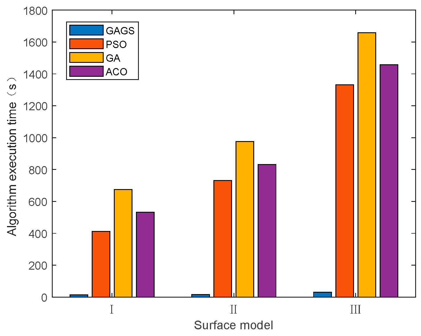
5.3. Comparison of Execution Time
The execution time of each algorithm under different surface models was compared. The deployment parameters of all algorithms are shown in Algorithm 1, and the comparison results are shown in
Figure 16. With the increase in the complexity of the surface model, the deployment time for all the algorithms has increased. However, the execution time of the GAGS algorithm is significantly shorter than that of the other three algorithms. It shows GAGS can effectively reduce the amount of calculation and the cost.
This is probably because swarm intelligence algorithms (PSO, GA, ACO) are greatly affected by initialization, which is highly random. It needs a large amount of calculation and has slow convergence in dealing with large-scale combination problems. However, GAGS is an algorithm based on the Greedy idea of grid scanning. It only needs to traverse all grid points once, which significantly reduces the time and space complexity. Moreover, the algorithm deployment scheme is unique and more stable.
6. Conclusions
To solve the WSN nodes coverage problem under real 3D terrain, this paper proposes a WSN deployment strategy for real 3D terrain coverage based on the Greedy algorithm with the DEM probability coverage model.
Firstly, DEM data is used to build a three-dimensional real terrain model of the area to be deployed, which can more truly reflect the characteristics of the area environment and make the deployment plan more visible. Secondly, a WSN probability coverage model based on DEM is established, which fully considers the impact of terrain shading and signal attenuation on the coverage model. Finally, a WSN deployment strategy based on the Greedy algorithm of grid scanning is proposed, which effectively improves the coverage of the monitoring area, dramatically reduces the computational complexity, and saves time.
The coverage performance of the proposed GAGS is verified through comparative experiments by comparison with the three traditional deployment algorithms of PSO, GA, and ACO. Experimental results show that for real terrain models with different complexity and coverage models with various parameters, the proposed GAGS can complete the coverage task with fewer nodes and has better coverage performance, faster execution, and more excellent stability.
Author Contributions
Conceptualization, W.F. and Y.Y.; methodology, W.F.; software, W.F. and G.H.; validation, W.F., Y.Y.; formal analysis, W.F.; investigation, W.F. and G.H.; resources, W.F. and Y.Y.; data curation, W.F. and G.H.; writing—original draft preparation, W.F.; writing—review and editing, Y.Y. and J.H.; visualization, W.F. and G.H.; supervision, Y.Y.; project administration, Y.Y.; funding acquisition, Y.Y. All authors have read and agreed to the published version of the manuscript.
Funding
This research was funded by National Natural Science Foundation of China, grant number 52007156, the Shanxi provincial Key Industry Innovation Chain—Industrial Field Project, grant number 2020ZDLGY15-02.
Institutional Review Board Statement
Not applicable.
Informed Consent Statement
Not applicable.
Conflicts of Interest
The authors declare no conflict of interest.
References
- Wang, Z.; Xie, H. Wireless Sensor Network Deployment of 3D Surface Based on Enhanced Grey Wolf Optimizer. IEEE Access 2020, 8, 57229–57251. [Google Scholar] [CrossRef]
- Kong, L.; Zhao, M.; Liu, X.-Y.; Lu, J.; Liu, Y.; Wu, M.-Y.; Shu, W. Surface Coverage in Sensor Networks. IEEE Trans. Parallel Distrib. Syst. 2014, 25, 234–243. [Google Scholar] [CrossRef]
- Liu, A.W.; Yang, S.; Sun, S.; Wei, S. A Node Deployment Optimization Method of WSN Based on Ant-Lion Optimization Algorithm. In Proceedings of the IEEE 4th International Symposium on Wireless Systems within the International Conferences on Intelligent Data Acquisition and Advanced Computing Systems (IDAACS-SWS), Lviv, Ukraine, 20–21 September 2018; pp. 88–92. [Google Scholar] [CrossRef]
- Xiang, T.; Wang, H.; Shi, Y. Hybrid WSN Node Deployment Optimization Strategy Based on CS Algorithm. In Proceedings of the IEEE 3rd Information Technology, Networking, Electronic and Automation Control Conference (ITNEC), Chengdu, China, 15–17 March 2019; pp. 621–625. [Google Scholar] [CrossRef]
- Arivudainambi, D.; Balaji, S.; Poorani, T.S. Sensor Deployment for Target Coverage in Underwater Wireless Sensor Network. In Proceedings of the 2017 International Conference on Performance Evaluation and Modeling in Wired and Wireless Networks (PEMWN), Paris, France, 28–30 November 2017; pp. 1–6. [Google Scholar] [CrossRef]
- Yang, R.; Fan, Y.; Zhao, N.; Cheng, Y. Improved Chemical Reaction Optimization algorithm for 3D complex surface coverage. In Proceedings of the IEEE 13th International Conference on Networking, Sensing, and Control (ICNSC), Mexico City, Mexico, 28–30 April 2016; pp. 1–6. [Google Scholar] [CrossRef]
- Mnasri, S.; Nasri, N.; Alrashidi, M.; Val, T. 3D Deployment Problem in Wireless Sensor Networks resolved by Genetic and Ant Colony Algorithms. In Proceedings of the 2020 International Conference on Computing and Information Technology (ICCIT-1441), Tabuk, Saudi Arabia, 9–10 September 2020; pp. 1–5. [Google Scholar] [CrossRef]
- Boufares, N.; Khoufi, I.; Minet, P.; Saidane, L.; Saied, Y.B. Three dimensional mobile wireless sensor networks redeployment based on virtual forces. In Proceedings of the International Wireless Communications and Mobile Computing Conference (IWCMC), Dubrovnik, Croatia, 24–28 August 2015; pp. 563–568. [Google Scholar] [CrossRef] [Green Version]
- Du, Y. Method for the Optimal Sensor Deployment of WSNs in 3D Terrain Based on the DPSOVF Algorithm. IEEE Access 2020, 8, 140806–140821. [Google Scholar] [CrossRef]
- Wang, Y.; Zhou, M.; Li, D.; Zhu, J.; Wang, Y. Deployment of Wireless Sensor Nodes in Coal Mine Based on Probabilistic Sensing Model. In Proceedings of the 2nd International Conference on Frontiers of Sensors Technologies (ICFST), Shenzhen, China, 14–16 April 2017; pp. 166–169. [Google Scholar] [CrossRef]
- Hossain, A.; Biswas, P.K.; Chakrabarti, S. Sensing Models and Its Impact on Network Coverage in Wireless Sensor Network. In Proceedings of the IEEE Region 10 and the Third international Conference on Industrial and Information Systems, Kharagpur, India, 8–10 December 2008; pp. 1–5. [Google Scholar] [CrossRef] [Green Version]
- Hao, Z.; Qu, N.; Dang, X.; Hou, J. RSS-Based Coverage Deployment Method under Probability Model in 3D-WSN. IEEE Access 2019, 7, 183091–183104. [Google Scholar] [CrossRef]
- Xiao, F.; Yang, X.; Yang, M.; Sun, L.; Wang, R.; Yang, P. Surface coverage algorithm in directional sensor networks for three-dimensional complex terrains. Tsinghua Sci. Technol. 2016, 21, 397–406. [Google Scholar] [CrossRef]
- Temel, S.; Unaldi, N.; Kaynak, O. On Deployment of Wireless Sensors on 3-D Terrains to Maximize Sensing Coverage by Utilizing Cat Swarm Optimization With Wavelet Transform. IEEE Trans. Syst. Man Cybern. Syst. 2014, 44, 111–120. [Google Scholar] [CrossRef]
- Zhao, M.-C.; Lei, J.; Wu, M.-Y.; Liu, Y.; Shu, W. Surface Coverage in Wireless Sensor Networks. In Proceedings of the IEEE INFOCOM 2009, Rio de Janeiro, Brazil, 19–25 April 2009; pp. 109–117. [Google Scholar] [CrossRef] [Green Version]
- Nespolo, R.; Neves, L.A.; Roberto, G.; Ribeiro, M.; Zanchetta do Nascimento, M.; Cansian, A. Method Based on Triangulation for Sensor Deployment on 3D Surfaces. In Proceedings of the 29th SIBGRAPI Conference on Graphics, Patterns and Images (SIBGRAPI), Sao Paulo, Brazil, 4–7 October 2016; pp. 136–143. [Google Scholar] [CrossRef]
- Zafer, M.; Senouci, M.R.; Aissani, M. On Coverage of 3D Terrains by Wireless Sensor Networks. In Proceedings of the 2019 Federated Conference on Computer Science and Information Systems (FedCSIS), Leipzig, Germany, 1–4 September 2019; pp. 501–504. [Google Scholar] [CrossRef] [Green Version]
- Boufares, N.; Saied, Y.B.; Saidane, L.A. Improved Distributed Virtual Forces Algorithm for 3D Terrains Coverage in Mobile Wireless Sensor Networks. In Proceedings of the IEEE/ACS 15th International Conference on Computer Systems and Applications (AICCSA), Aqaba, Jordan, 28 October–1 November 2018; pp. 1–8. [Google Scholar] [CrossRef]
- Saha, S.; Saikia, M. Wireless Sensor Node Deployment Strategy in Hilly Terrains for Maximizing Area of Coverage. In Proceedings of the 4th International Conference on Computing Communication and Automation (ICCCA), Greater Noida, India, 14–15 December 2018; pp. 1–6. [Google Scholar] [CrossRef]
- Felamban, M.; Shihada, B.; Jamshaid, K. Optimal Node Placement in Underwater Wireless Sensor Networks. In Proceedings of the IEEE 27th International Conference on Advanced Information Networking and Applications (AINA), Barcelona, Spain, 25–28 March 2013; pp. 492–499. [Google Scholar] [CrossRef] [Green Version]
- Geospatial Data Cloud. Available online: http://www.gscloud.cn/ (accessed on 8 September 2020).
Figure 1.
Contour model, GRID model, TIN model.
Figure 1.
Contour model, GRID model, TIN model.
Figure 2.
Comparison of DEM data volume and modeling accuracy.
Figure 2.
Comparison of DEM data volume and modeling accuracy.
Figure 3.
Schematic representation of the effect of terrain shading on model coverage.
Figure 3.
Schematic representation of the effect of terrain shading on model coverage.
Figure 4.
Estimation of the elevation value of the node in any sensing direction.
Figure 4.
Estimation of the elevation value of the node in any sensing direction.
Figure 5.
Elevation value point coverage criterion in the direction of node perception.
Figure 5.
Elevation value point coverage criterion in the direction of node perception.
Figure 6.
The relationship curve between coverage rate and distance under different attenuation factors.
Figure 6.
The relationship curve between coverage rate and distance under different attenuation factors.
Figure 7.
Node deployment under simple terrain model.
Figure 7.
Node deployment under simple terrain model.
Figure 8.
Node deployment under the general terrain model.
Figure 8.
Node deployment under the general terrain model.
Figure 9.
Node deployment under complex terrain model.
Figure 9.
Node deployment under complex terrain model.
Figure 10.
Coverage comparison histogram.
Figure 10.
Coverage comparison histogram.
Figure 11.
Node deployment after increasing the coverage model attenuation factor.
Figure 11.
Node deployment after increasing the coverage model attenuation factor.
Figure 12.
Histogram of algorithm coverage comparison after increasing the coverage model attenuation factor.
Figure 12.
Histogram of algorithm coverage comparison after increasing the coverage model attenuation factor.
Figure 13.
Node deployment results after reducing the coverage threshold.
Figure 13.
Node deployment results after reducing the coverage threshold.
Figure 14.
Histogram of algorithm coverage comparison after reducing the coverage threshold.
Figure 14.
Histogram of algorithm coverage comparison after reducing the coverage threshold.
Figure 15.
Line chart of algorithm coverage ratio comparison under preset coverage ratio.
Figure 15.
Line chart of algorithm coverage ratio comparison under preset coverage ratio.
Figure 16.
Comparison histogram of the execution time required for each algorithm to complete the deployment plan under different surface models.
Figure 16.
Comparison histogram of the execution time required for each algorithm to complete the deployment plan under different surface models.
Table 1.
The impact of terrain shading on corresponding grid points.
Table 1.
The impact of terrain shading on corresponding grid points.
| The Number of Grid Points | Impact of Terrain Shading Pteri |
|---|
| grid 1 | 1 |
| grid 2 | 0 |
| grid 3 | 1 |
| grid 4 | 0 |
| grid 5 | 1 |
| grid 6 | 0 |
Table 2.
Simulation parameters.
Table 2.
Simulation parameters.
| Parameter | Value |
|---|
| Projection Area of Monitoring Area | 600 × 600 m2 |
| Node Perceived Radius R | 5 m |
| Uncertain perception radius r | 1 m |
| Attenuation factor α, β | 0.5 |
| Grid length g | 12 m |
| Coverage threshold value φ | 0.8 |
| Preset coverage rate | 1 |
| Publisher’s Note: MDPI stays neutral with regard to jurisdictional claims in published maps and institutional affiliations. |
© 2021 by the authors. Licensee MDPI, Basel, Switzerland. This article is an open access article distributed under the terms and conditions of the Creative Commons Attribution (CC BY) license (https://creativecommons.org/licenses/by/4.0/).


