
Congestion Prediction in FPGA Using Regression Based Learning Methods


Abstract
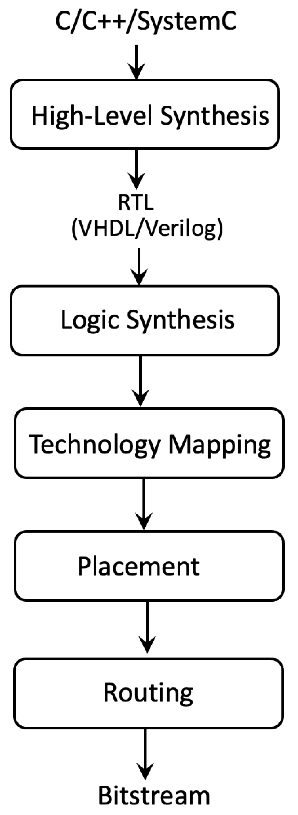
:1. Introduction
2. Related Literature
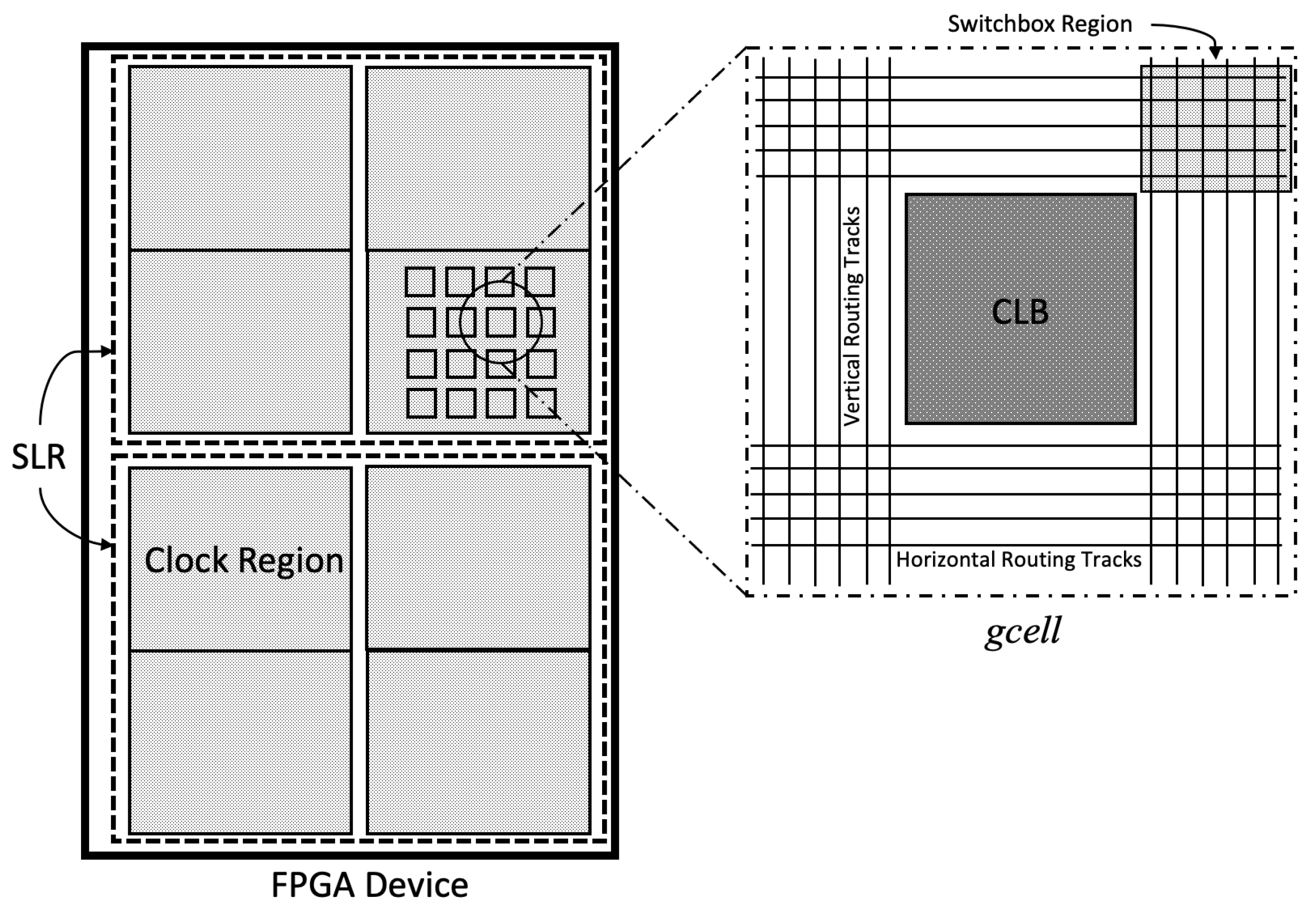
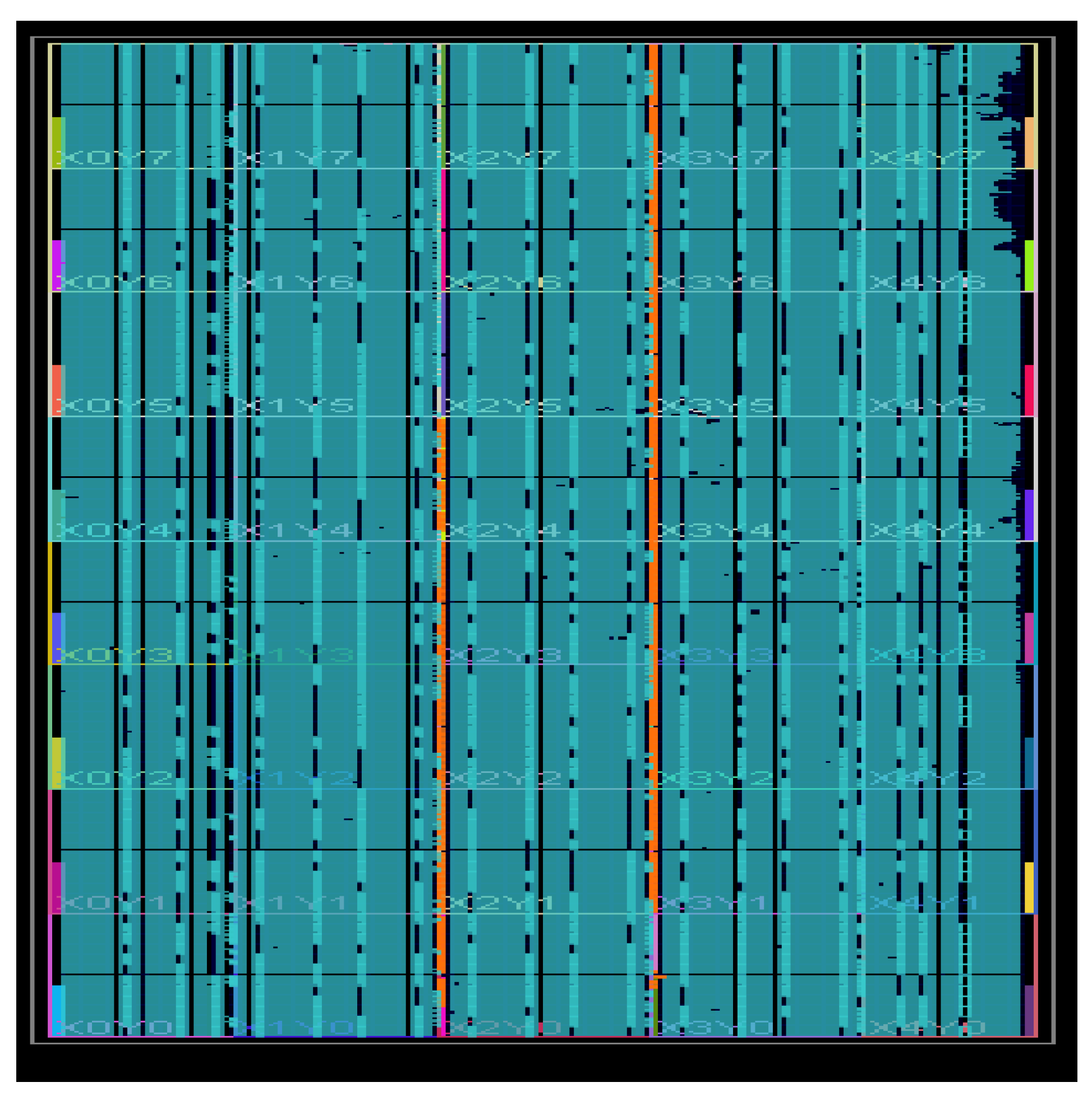
3. FPGA Architecture Description
4. FPGA Routing Congestion Prediction Framework
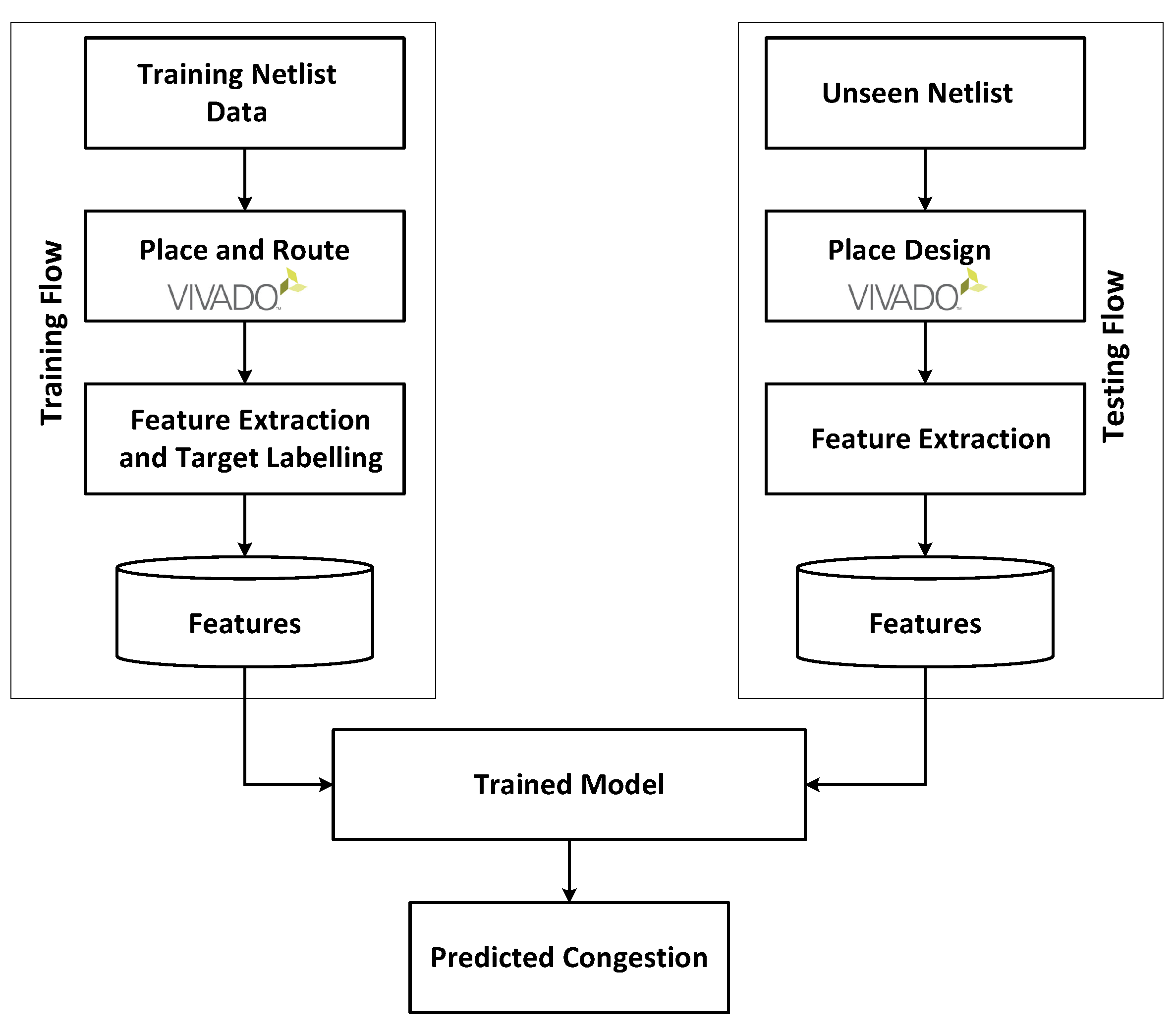
4.1. Prediction Framework Flow
4.2. Feature Extraction for Placed Netlists
- Number of Utilized Cells (): A Xilinx Ultrascale+ CLB slice consists of four different types of cells, viz., LUT, Flip-Flops, Multiplexers, and Carry Chains. One CLB has multiple units of each cell type. The number of cells utilized by a net inside each CLB tile plays an important role in measuring the congestion around each CLB block. When more and more cells within a CLB tile are used, more wiring resources would clearly be required to interconnect them. Based on this intuition, we calculated the number of cells used inside each of the CLB slices and used it as a vital parameter in our ML based prediction model. If more cells are used, the probability of congestion around the CLB increases proportionately.
- Number of Pins (): Each cell in the CLB slice contains a certain number of pins. For example, a H6LUT contains eight pins (6 inputs and 2 outputs), a mux contains four pins, and a flip-flop contains five pins. When pins are connected to wires, they are an indicator of local congestion inside the CLB tile. We keep track of the number of used pins in each CLB tile as a useful feature.
- Number of incoming/outgoing nets ( and ): If a net has pins spread across multiple CLB slices all over the FPGA, it can be considered as a multi-CLB net. Each multi-CLB net can be covered by a bounding box. The number of multi-CLB incoming and outgoing nets passing through a CLB slice provides us with the number of bounding boxes that crossed that particular CLB. The greater the number of bounding boxes passing through a CLB slice, the higher the congestion results. Hence, the number of bounding boxes passing through a CLB slice is an important feature for estimating the routing congestion around it.
- Number of Local/Buried nets (): Local nets or buried nets represent nets where all the cells are present in the same CLB slice. Even if all the cells are placed inside one CLB, the wires use the routing tracks present in the gcell to route the signals. Hence, this feature also contributes to routing congestion in the gcell.
- Location of the gcell inside the FPGA ( and ): The absolute location of a gcell is not very relevant. When a group of cells is placed in a localized region, every cell in the group impacts congestion of other cells in the group. Analysis shows that the location of a tile inside the FPGA plays one of the crucial roles in routing congestion estimation, as a tile in an already congested region will experience greater congestion. This is because the neighboring gcells of a gcell play an important role in the congestion. Gcells which are surrounded by high cell density or high pin density gcells will have high routing congestion.
- LUT () and Flip Flop () Utilization: Each CLB or gcell consists of 8 LUTs and 16 FFs. This feature represents the percentage of LUTs and FFs used inside a gcell. These features also contribute to congestion, but their effect is very low than compared to the other features discussed above.
- Super Logic Regionid;
- Placement of logic within a specific clock-region in an SLR;
- CLE type;
- Total number of LUTs, Flip-Flops, and Multiplexors in a CLB.
4.3. Creation and Training of Regression Model
- Linear Regression: Linear regression is a method to find relationship between two continuous variables, where one is independent and the other is dependent. Linear regression tries to create a statistical relationship which may not be always deterministic. Linear regression tries to obtain a straight line which shows the relationship between the independent and the dependent variable. For most of the linear regression models, the error is measured by using least squared error. A linear regression line has an equation of the form , where X is the independent variable and Y is the dependent variable. The slope of the line is b, and a is the intercept, which are both determined during training of the model.
- Random Forest Regression: Random forest is a supervised learning method that uses ensemble methods for learning. Ensemble learning is a technique that combines multiple weak learners to create a strong learner. In random forest, these weak learners are decision trees. The outputs from the individual learners are averaged in order to generate the final output. Random forest belongs to the bagging class of learners where, during training, data samples are selected at random without replacement. Bagging makes each model run independently and then aggregates the outputs at the end without preference to any model. Due to the introduction of the bagging method, the chances of overfit are lower in random forest. Random forest is a very fast method of training because each tree can be trained in parallel, and the inputs and outputs of each individual tree are not related to another. To summarize, the Random Forest Algorithm merges the output of multiple decision trees to generate the final output.
- Multivariate Adaptive Regression Splines (MARS): Multivariate adaptive regression splines (MARS) [26] is an algorithm that automatically creates a piecewise linear model which creates a non-linear model by combining multiple small linear functions known as steps. In MARS, non-linearity is introduced by using step functions. There are no polynomial terms in the MARS equation. Equation (2) shows the linear step wise equation:MARS is an adaptive procedure for regression and is well suited for high-dimensional problems (i.e., a large number of inputs). The bends in the step functions are known as “knots”. If there are multiple knots present in the MARS equation, it may result in overfitting.
- Multi Layer Perceptron based Regression (MLP: MLP based regression models are made up of multiple perceptrons also known as neurons. This type of model falls into the feedforward class of artificial neural networks. Generally, ANNs are used for classification. However, they can also be used for regression. MLP based models are trained using backpropagation algorithm. Each network consists of an input layer of neurons, few hidden layers, and an output layer. The output of each neuron is linear. In order to make the output non-linear and to simulate the real world behavior, activation functions such as “tanh” and “sigmoid” are added.
4.4. Generation of Training Data
5. Experiments and Results
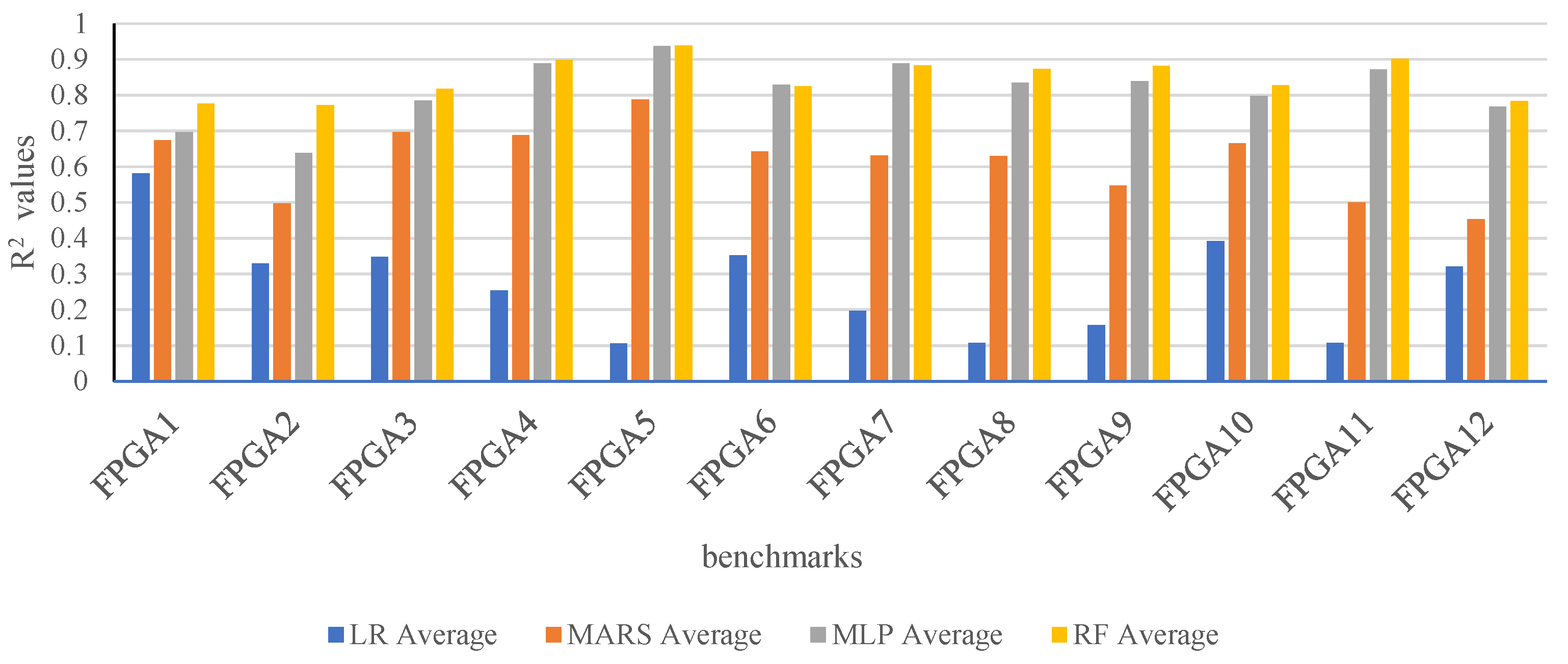
5.1. Analysis of Accuracy
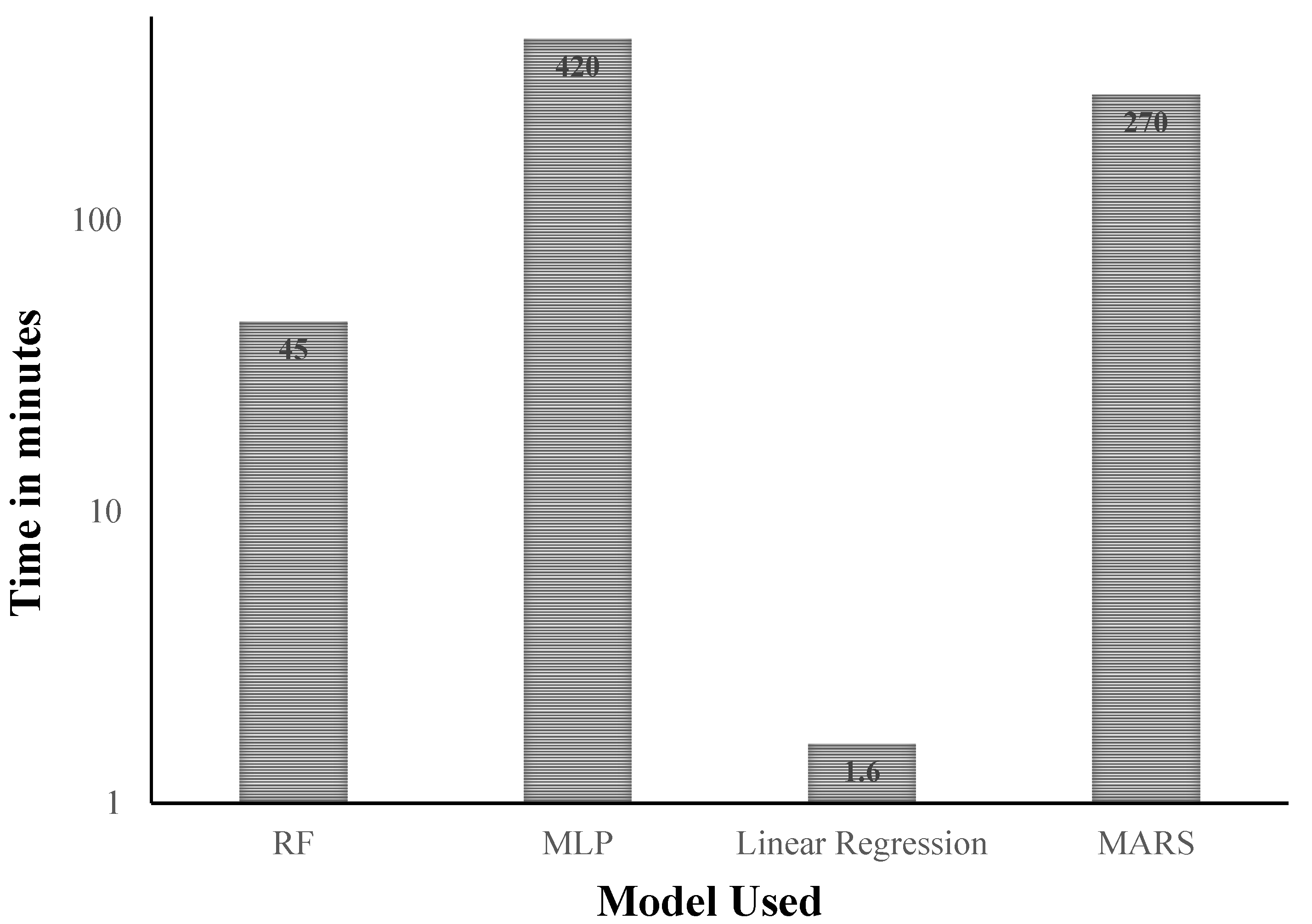
5.2. Discussion
6. Conclusions
- The methodology is to generate a robust congestion prediction model that makes use of easily obtained features from a placed design. The model exhibits an average MAPE of and maximum value of on completely unseen designs. These are the best known and tightest results.
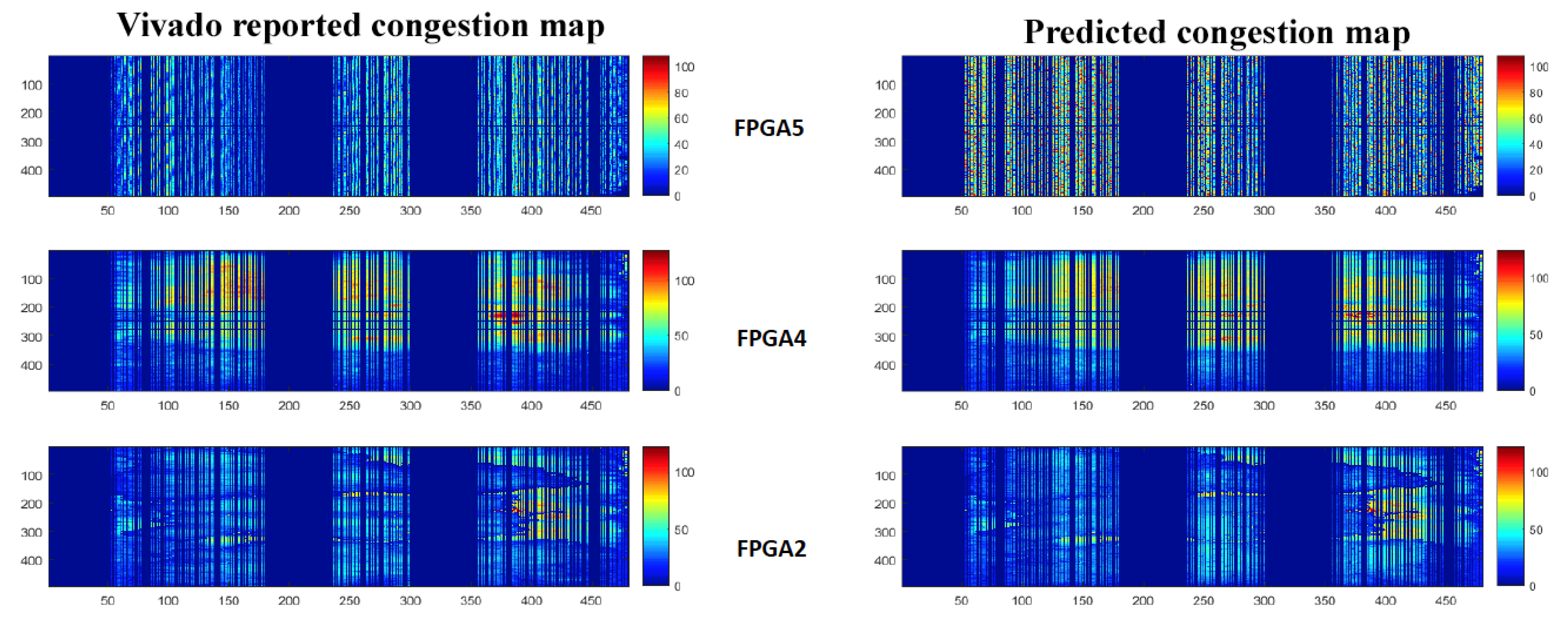
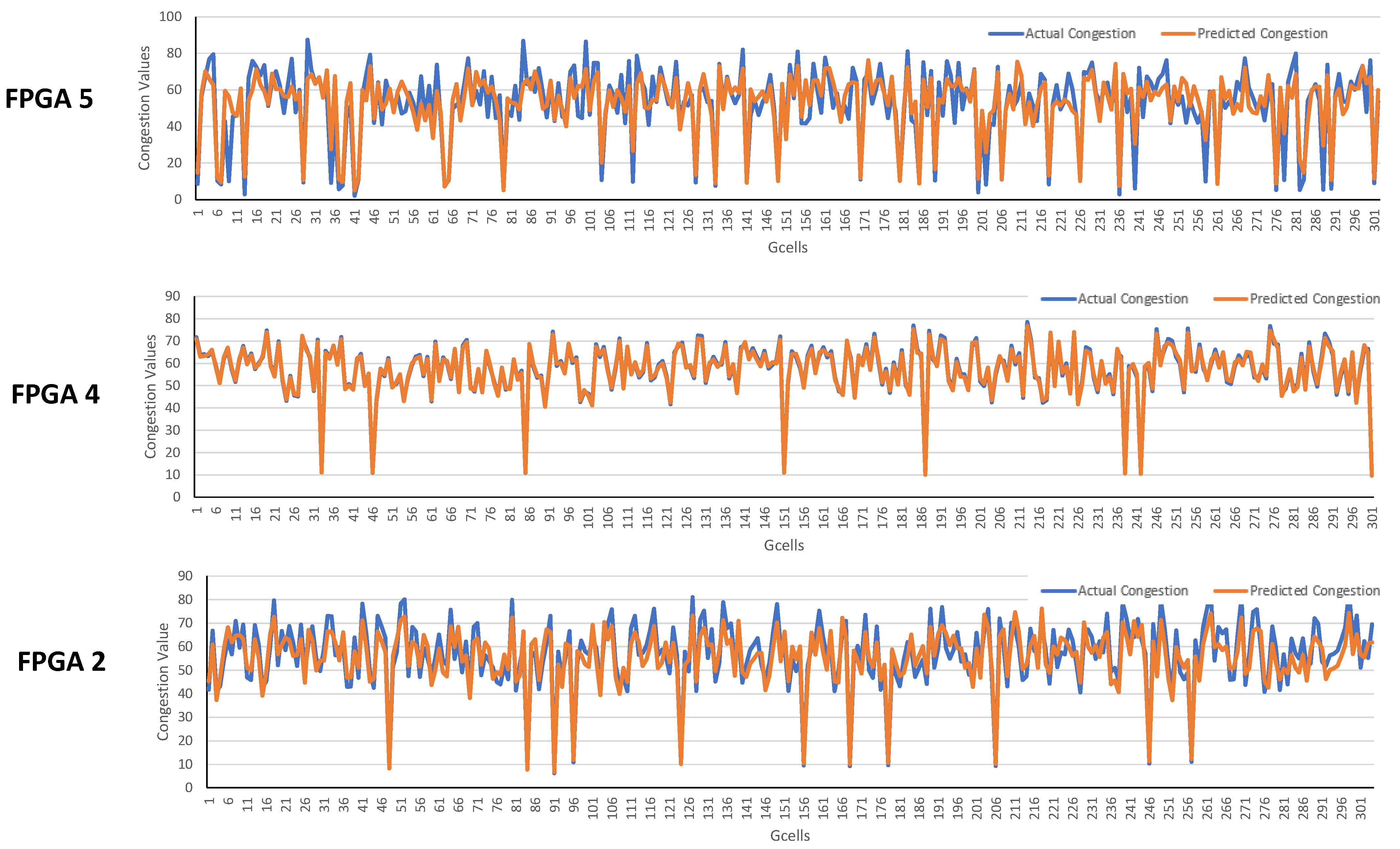
- The post-placement congestion prediction values provide accurate congestion in horizontal and vertical channels. The report is consistent with the post-route congestion estimation that Xilinx Vivado tools provide after routing. This enables easy integration of our model based prediction in the Xilinx Vivado tool flow.
- Our methodology demonstrates that a carefully crafted set of features based model can be trained with a relatively small set of training data. Our models were trained with about 160K databins derived out of four benchmark examples. The test data were completely unseen data.
Author Contributions
Funding
Data Availability Statement
Conflicts of Interest
References
- Xu, X.; Matsunawa, T.; Nojima, S.; Kodama, C.; Kotani, T.; Pan, D.Z. A Machine Learning Based Framework for Sub-Resolution Assist Feature Generation. In Proceedings of the International Symposium on Physical Design (ISPD 2016), Santa Rosa, CA, USA, 3–6 April 2016; ACM: New York, NY, USA, 2016; pp. 161–168. [Google Scholar] [CrossRef]
- Yanghua, Q.; Ng, H.; Kapre, N. Boosting convergence of timing closure using feature selection in a Learning-driven approach. In Proceedings of the 2016 26th International Conference on Field Programmable Logic and Applications (FPL), Lausanne, Switzerland, 29 August–2 September 2016; pp. 1–9. [Google Scholar] [CrossRef]
- Kapre, N.; Ng, H.; Teo, K.; Naude, J. InTime: A Machine Learning Approach for Efficient Selection of FPGA CAD Tool Parameters. In Proceedings of the 2015 ACM/SIGDA International Symposium on Field-Programmable Gate Arrays, Monterey, CA, USA, 22–24 February 2015; ACM: New York, NY, USA, 2015; pp. 23–26. [Google Scholar] [CrossRef]
- Chang, W.; Lin, C.; Mu, S.; Chen, L.; Tsai, C.; Chiu, Y.; Chao, M.C. Generating Routing-Driven Power Distribution Networks With Machine-Learning Technique. IEEE Trans. Comput. Aided Des. Integr. Circuits Syst. 2017, 36, 1237–1250. [Google Scholar] [CrossRef]
- Chan, W.T.J.; Ho, P.H.; Kahng, A.B.; Saxena, P. Routability Optimization for Industrial Designs at Sub-14Nm Process Nodes Using Machine Learning. In Proceedings of the 2017 ACM on International Symposium on Physical Design, Portland, OR, USA, 19–22 March 2017; ACM: New York, NY, USA, 2017; pp. 15–21. [Google Scholar] [CrossRef]
- Zhou, Q.; Wang, X.; Qi, Z.; Chen, Z.; Zhou, Q.; Cai, Y. An accurate detailed routing routability prediction model in placement. In Proceedings of the 2015 6th Asia Symposium on Quality Electronic Design (ASQED), Kuala Lumpur, Malaysia, 4–5 August 2015; pp. 119–122. [Google Scholar] [CrossRef]
- Tabrizi, A.F.; Darav, N.K.; Xu, S.; Rakai, L.; Bustany, I.; Kennings, A.; Behjat, L. A Machine Learning Framework to Identify Detailed Routing Short Violations from a Placed Netlist. In Proceedings of the 55th Annual Design Automation Conference, San Francisco, CA, USA, 24–29 June 2018; ACM: New York, NY, USA, 2018; pp. 48:1–48:6. [Google Scholar] [CrossRef]
- Liu, W.; Wei, Y.; Sze, C.; Alpert, C.J.; Li, Z.; Li, Y.-L.; Viswanathan, N. Routing congestion estimation with real design constraints. In Proceedings of the 2013 50th ACM/EDAC/IEEE Design Automation Conference (DAC), Austin, TX, USA, 29 May–7 June 2013; pp. 1–8. [Google Scholar]
- Shojaei, H.; Davoodi, A.; Linderoth, J.T. Congestion analysis for global routing via integer programming. In Proceedings of the 2011 IEEE/ACM International Conference on Computer-Aided Design (ICCAD), San Jose, CA, USA, 7–10 November 2011; pp. 256–262. [Google Scholar] [CrossRef] [Green Version]
- Saeedi, M.; Zamani, M.S.; Jahanian, A. Evaluation, Prediction and Reduction of Routing Congestion. Microelectron. J. 2007, 38, 942–958. [Google Scholar] [CrossRef]
- Kannan, P.; Balachandran, S.; Bhatia, D. fGREP—Fast Generic Routing Demand Estimation for Placed FPGA Circuits. In Field-Programmable Logic and Applications; Brebner, G., Woods, R., Eds.; Springer: Berlin/Heidelberg, Germany, 2001; pp. 37–47. [Google Scholar]
- Balachandran, S.; Kannan, P.; Bhatia, D. On metrics for comparing interconnect estimation methods for FPGAs. IEEE Trans. Very Large Scale Integr. (VLSI) Syst. 2004, 12, 381–385. [Google Scholar] [CrossRef]
- Kannan, P.; Bhatia, D. Interconnect Estimation for FPGAs. IEEE Trans. Comput. Aided Des. Integr. Circuits Syst. 2006, 25, 1523–1534. [Google Scholar] [CrossRef]
- Maarouf, D.; Alhyari, A.; Abuowaimer, Z.; Martin, T.; Gunter, A.; Grewal, G.; Areibi, S.; Vannelli, A. Machine-Learning Based Congestion Estimation for Modern FPGAs. In Proceedings of the 2018 28th International Conference on Field Programmable Logic and Applications (FPL), Dublin, Ireland, 27–31 August 2018; pp. 427–4277. [Google Scholar] [CrossRef]
- Pui, C.; Chen, G.; Ma, Y.; Young, E.F.Y.; Yu, B. Clock-aware ultrascale FPGA placement with machine learning routability prediction: (Invited paper). In Proceedings of the 2017 IEEE/ACM International Conference on Computer-Aided Design (ICCAD), Irvine, CA, USA, 13–16 November 2017; pp. 929–936. [Google Scholar] [CrossRef]
- Vivado Development Team. Xilinx Vivado. Available online: https://www.xilinx.com/products/design-tools/vivado.html (accessed on 17 August 2021).
- Yang, S.; Gayasen, A.; Mulpuri, C.; Reddy, S.; Aggarwal, R. Routability-Driven FPGA Placement Contest. In Proceedings of the 2016 on International Symposium on Physical Design, Santa Rosa, CA, USA, 3–6 April 2016; ACM: New York, NY, USA, 2016; pp. 139–143. [Google Scholar] [CrossRef]
- Balachandran, S.; Bhatia, D. A-priori Wirelength and Interconnect Estimation based on Circuit Characteristics. IEEE Trans. Comput. Aided Des. Integr. Circuits Syst. 2005, 24, 1054–1065. [Google Scholar] [CrossRef]
- Zhao, J.; Liang, T.; Sinha, S.; Zhang, W. Machine Learning Based Routing Congestion Prediction in FPGA High-Level Synthesis. In Proceedings of the 2019 Design, Automation Test in Europe Conference Exhibition (DATE), Florence, Italy, 25–29 March 2019; pp. 1130–1135. [Google Scholar] [CrossRef] [Green Version]
- Xilinx Ultrascale+ Product Details. Available online: https://www.xilinx.com/support/documentation/product-briefs/virtex-ultrascale-plus-product-brief.pdf (accessed on 17 August 2021).
- Large FPGA Methodology Guide, Including Stacked Silicon Interconnect (SSI) Technology. Available online: https://www.xilinx.com/support/documentation/sw_manuals/xilinx14_7/ug872_largefpga.pdf (accessed on 17 August 2021).
- Xilinx Architecture Terminology. Available online: https://www.rapidwright.io/docs/Xilinx_Architecture.html (accessed on 17 August 2021).
- Comet ML Supercharging Machine Learning Tool. Available online: www.comet.ml (accessed on 17 August 2021).
- ELI5 Tool. Available online: https://eli5.readthedocs.io/en/latest/ (accessed on 17 August 2021).
- Amazon SageMaker Machine Learning for Every Data Scientist and Develope. Available online: https://aws.amazon.com/sagemaker/l (accessed on 17 August 2021).
- Friedman, J.H. Multivariate Adaptive Regression Splines. Ann. Statist. 1991, 19, 1–67. [Google Scholar] [CrossRef]
- Al-Hyari, A.; Abuowaimer, Z.; Martin, T.; Gréwal, G.; Areibi, S.; Vannelli, A. Novel Congestion-Estimation and Routability-Prediction Methods Based on Machine Learning for Modern FPGAs. ACM Trans. Reconfigurable Technol. Syst. 2019, 12. [Google Scholar] [CrossRef] [Green Version]
- Data Repository for Machine Learning Based Congestion Estimation. Available online: https://personal.utdallas.edu/~dinesh/Data/ (accessed on 17 August 2021).


| 2 | 8 | 6 | 2 | 7 | 3 | 86 | 12.5 | 6.25 |
| 8 | 41 | 33 | 8 | 24 | 4 | 86 | 62.5 | 18.75 |
| 5 | 22 | 17 | 5 | 19 | 4 | 88 | 25 | 18.75 |
| 4 | 21 | 17 | 4 | 18 | 4 | 90 | 25 | 12.5 |
| Number of Units Used | ||||
|---|---|---|---|---|
| Design Name | FF | LUT | BRAM | Databins |
| EXAMPLE 1 | 1260 | 1968 | 2 | 325 |
| EXAMPLE 2 | 237,012 | 289,036 | 384 | 44,565 |
| EXAMPLE 3 | 175,585 | 244,435 | 495 | 46,161 |
| EXAMPLE 4 | 344,295 | 447,021 | 1114 | 66,728 |
| Total | 157,779 | |||
| LUT | FF | BRAM |
|---|---|---|
| 537,600 | 1,075,200 | 1728 |
| Benchmark | # of Nets | # of Cells | #of Databins |
|---|---|---|---|
| FPGA1 | 104,061 | 103,958 | 10,161 |
| FPGA2 | 165,380 | 163,780 | 17,326 |
| FPGA3 | 424,679 | 416,877 | 40,332 |
| FPGA4 | 426,857 | 419,056 | 42,281 |
| FPGA5 | 431,127 | 423,332 | 50,115 |
| FPGA6 | 658,627 | 649,435 | 62,369 |
| FPGA7 | 684,910 | 675,699 | 66,194 |
| FPGA8 | 722,314 | 714,515 | 66,814 |
| FPGA9 | 876,754 | 867,954 | 67,200 |
| FPGA10 | 786,967 | 778,207 | 64,821 |
| FPGA11 | 822,378 | 816,034 | 66,522 |
| FPGA12 | 966,389 | 959,025 | 66,063 |
| Random Forest | MLP | |||
|---|---|---|---|---|
| Design | Vertical | Horizontal | Vertical | Horizontal |
| FPGA1 | 1.689 | 4.649 | 4.894 | 1.910 |
| FPGA2 | 2.186 | 1.721 | 2.159 | 2.805 |
| FPGA3 | 3.370 | 2.998 | 3.237 | 3.653 |
| FPGA4 | 4.638 | 3.949 | 4.117 | 4.746 |
| FPGA5 | 5.311 | 4.870 | 4.965 | 5.250 |
| FPGA6 | 3.591 | 3.634 | 3.694 | 3.379 |
| FPGA7 | 4.745 | 4.847 | 4.650 | 4.760 |
| FPGA8 | 4.498 | 3.886 | 4.349 | 5.395 |
| FPGA9 | 5.263 | 6.103 | 4.863 | 5.467 |
| FPGA10 | 3.868 | 3.859 | 4.117 | 4.169 |
| FPGA11 | 5.373 | 5.318 | 6.157 | 5.859 |
| FPGA12 | 7.994 | 5.318 | 5.365 | 8.205 |
| Design | MLP | RF | Actual Routing |
|---|---|---|---|
| Seconds | Minutes | ||
| FPGA1 | 15.023 | 0.955 | 15 |
| FPGA2 | 73.586 | 1.542 | 24 |
| FPGA3 | 143.336 | 3.761 | 24 |
| FPGA4 | 226.608 | 4.005 | 36 |
| FPGA5 | 276.508 | 5.038 | 66 |
| FPGA6 | 266.521 | 6.165 | 84 |
| FPGA7 | 427.346 | 6.583 | 114 |
| FPGA8 | 368.471 | 5.985 | 132 |
| FPGA9 | 411.258 | 5.896 | 141 |
| FPGA10 | 189.253 | 5.854 | 150 |
| FPGA11 | 288.107 | 6.309 | 168 |
| FPGA12 | 221.788 | 6.442 | 192 |
Publisher’s Note: MDPI stays neutral with regard to jurisdictional claims in published maps and institutional affiliations. |
© 2021 by the authors. Licensee MDPI, Basel, Switzerland. This article is an open access article distributed under the terms and conditions of the Creative Commons Attribution (CC BY) license (https://creativecommons.org/licenses/by/4.0/).
Share and Cite
Goswami, P.; Bhatia, D. Congestion Prediction in FPGA Using Regression Based Learning Methods. Electronics 2021, 10, 1995. https://doi.org/10.3390/electronics10161995
Goswami P, Bhatia D. Congestion Prediction in FPGA Using Regression Based Learning Methods. Electronics. 2021; 10(16):1995. https://doi.org/10.3390/electronics10161995
Chicago/Turabian StyleGoswami, Pingakshya, and Dinesh Bhatia. 2021. "Congestion Prediction in FPGA Using Regression Based Learning Methods" Electronics 10, no. 16: 1995. https://doi.org/10.3390/electronics10161995
APA StyleGoswami, P., & Bhatia, D. (2021). Congestion Prediction in FPGA Using Regression Based Learning Methods. Electronics, 10(16), 1995. https://doi.org/10.3390/electronics10161995