An Efficient FPGA-Based Convolutional Neural Network for Classification: Ad-MobileNet

Abstract

Convolutional Neural Networks (CNN) continue to dominate research in the area of hardware acceleration using Field Programmable Gate Arrays (FPGA), proving its effectiveness in a variety of computer vision applications such as object segmentation, image classification, face detection, and traffic signs recognition, among others. However, there are numerous constraints for deploying CNNs on FPGA, including limited on-chip memory, CNN size, and configuration parameters. This paper introduces Ad-MobileNet, an advanced CNN model inspired by the baseline MobileNet model. The proposed model uses an Ad-depth engine, which is an improved version of the depth-wise separable convolution unit. Moreover, we propose an FPGA-based implementation model that supports the Mish, TanhExp, and ReLU activation functions. The experimental results using the CIFAR-10 dataset show that our Ad-MobileNet has a classification accuracy of 88.76% while requiring little computational hardware resources. Compared to state-of-the-art methods, our proposed method has a fairly high recognition rate while using fewer computational hardware resources. Indeed, the proposed model helps to reduce hardware resources by more than 41% compared to that of the baseline model.

1. Introduction

Convolutional neural networks (CNNs) are widely used in research areas, particularly in computer vision applications such as facial recognition, image classification, weather forecasting, and object detection. CNNs built in recent years have become deeper [1,2,3,4,5,6,7,8], as is the trend in the research field. The deeper the CNN, the harder it is to implement as a hardware accelerator on an FPGA-based embedded board, with comparable processing speed and precision.

For a suitable FPGA-based deployment, shallow and lightweight CNN models, such as MobileNet [9,10] and ShuffleNet [11] are good candidates. However, we are still concerned about maintaining the highest possible precision and processing power. To address this issue, we propose Ad-MobileNet, a network based on the standard MobileNet model that, while minimizing the computational cost of hardware resources, achieves a significant recognition rate that outperforms many leading FPGA-based implementations.

Ad-MobileNet differs from the baseline MobileNet model. Indeed, in this model, we propose an Ad-depth unit, which replaces the traditional depthwise separable convolution. This unit is better suited for hardware implementation because it offers improved accuracy without significantly affecting the computational cost of hardware resources. In addition, as will be demonstrated later, some layers having a negligible negative impact on the recognition rate have been removed to facilitate hardware implementation. Third, besides accuracy, the choice of activation function also has an impact on performance. Simple activation functions, such as sigmoid [12,13], rectified linear unit (ReLU) [14], and Tanh [15,16], are preferred for hardware implementation. However, to improve classification accuracy, MobileNet relies on various alternative activation functions that tend to work better on deep models. Therefore, we have also extended the supported activation function set with ReLU [14], Tanh Exponential (TanhExp) [17,18], and Mish [19].

In this paper, we propose Ad-MobileNet, a hardware-accelerated version of MobileNet. For this FPGA-based model, we decided to use the floating-point representation to preserve the precision of the classification. However, the piecewise linear method (PWL) is used to approximate nonlinear activations, thereby reducing the computational resources. The remainder of this paper is organized as follows. Section 2 presents a state-of-the-art analysis of the CNN implementations on FPGAs. Section 3 describes the MobileNet model and the depthwise separable convolution unit. Then, in Section 4, we introduce the proposed Ad-MobileNet model. Section 5 describes the development methodology and hardware implementation of the CNN on an FPGA using the CIFAR-10 dataset as an example. We also detail the activation functions ReLU, TanhExp, and Mish, as well as the piecewise linear approximation (PWL) method. Section 6 presents the experimental results of the hardware implementation while varying the activation function, followed by a performance comparison with the state-of-the-art in Section 7. Section 8 concludes the paper.

2. Related Work

Convolution neural networks (CNNs) require intensive CPU operations and memory bandwidth, which causes general CPUs to fail to achieve the desired performance levels. Consequently, hardware accelerators based on application-specific integrated circuits (ASICs) and field programmable gate arrays (FPGAs) have been employed to improve the throughput of CNNs. Many studies have focused on FPGA-based CNN topologies to improve processing performance. Indeed, FPGAs provide flexibility, high throughput, fine-grain parallelism, and energy efficiency. However, implementing hardware-accelerated CNNs at the edge is a complex task owing to limitations in memory resources, computing power, and power consumption restrictions.

Many recent techniques have been used to improve the acceleration performance of CNNs on FPGAs [20,21,22]. FPGAs can achieve a moderate performance with lower power consumption. However, FPGAs have relatively limited memory and computing resources. For this reason, several approaches focus on the trade-offs between precision, processing power, and hardware resources when proposing building blocks for CNNs. For example, in [23], the authors proposed a processing element (PE) in which the built-in multiplier accumulator (MAC) was replaced by a Wallace Tree-based Multiplier. In [24], the authors proposed an optimized memory access by combining FIFO and ping-pong memory operations on a Xilinx ZCU102 device. In contrast, in [20], the authors proposed a pipelined parallel architecture with a standard ReLU as an activation function to improve the computational efficiency.

Numerous studies have been conducted at a coarse grain level to further enhance the CNN inference speed. In [25], the authors proposed a 23-layer SqueezeNet model, in which each layer of the CNN was optimized and implemented separately on a Xilinx VC709 FPGA board. However, the experiments showed a low recognition rate of 79% for the top-five accuracy. In [26], the authors suggested a reduced-parameter CNN model that reduced the size of the network model. Thus, they fitted smaller convolutional kernels on a Xilinx Zynq XC7Z020 FPGA device. In particular, in [27], two dedicated computing engines, Conv and Dwcv, were developed for pointwise convolution and depthwise convolution, respectively. Their CNN model used the standard ReLU as the activation function. Their experiments showed a low recognition rate of 68% top-1 accuracy on ImageNet, whereas they used more than 2070 DSPs. The authors in [28] proposed the Winograd fast convolution algorithm (WFCA), which can lower the complexity by reducing multiplications. Based on the ZYNQ FPGA device, the authors of [21] created a CNN accelerator that can accelerate both standard and depthwise separable convolutions. While still using the standard ReLU as the activation function, they used 95% of the available DSPs.

3. Background

The CNN has a multilayered structure, composed of a convolution layer, to extract feature maps from an input image, an activation function that decides the features to be transferred between neurons, a pooling layer to reduce the spatial size of feature maps, thus the number of parameters and computational load (it also prevents overfitting during the learning process), and a fully connected layer that classifies using the extracted features. There are different types of CNN architectures with different shapes and sizes. Some are deep models, such as GoogLeNet [2], DenseNet [4], VGG [29], and ResNet [30], whereas others are shallow and light CNNs, such as MobileNet [9], an improved model using SigmaH as the activation function [31], and ShuffleNet [11].

3.1. Convolution Layer

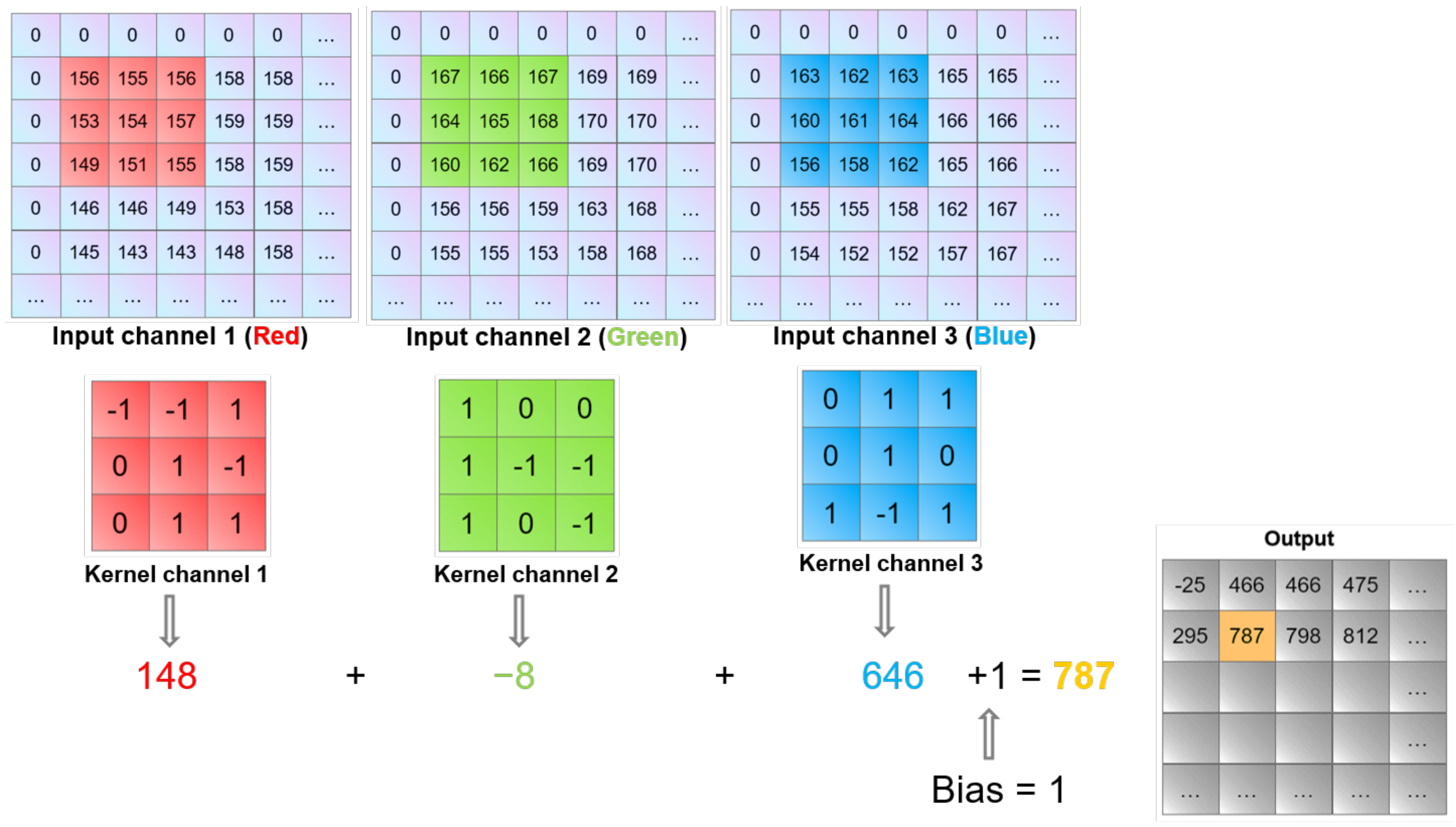
The convolutional layer employs a collection of learnable filters to detect essential characteristics in the image data. The convolution is a linear operation consisting of the multiplication of a two-dimensional array called a filter with an input array. The filter, which is smaller than the input data, is applied multiple times to different locations of the input array, resulting in a two-dimensional array called a feature map. The element-wise multiplication is summed, resulting in a single value, operation performed by a multiply accumulate (MACC) mathematical operator. Figure 1 represents the multiplication of the receptive region of the inputs by the filter, kernel or matrix of weights. A bias value is added to the sum of the weighted inputs. The figure represents the convolution process for a three-dimensional input. Equation (1) depicts a function that calculates the output size of the feature map.

$$Outpu{t}_{size}=\frac{Inpu{t}_{width}-Kerne{l}_{size}+2\times Padding}{Stride}+Bias.$$

(1)

where $kernel$ is a filter that is used to extract image features, $Padding$ is the number of pixels that are added to the image when processed by a CNN kernel, and $Stride$ is the number of pixels shifted across the input matrix.

Generally, this operation has no limit, making it difficult for the neuron to decide whether to fire. Thus, using an activation function on the accumulated sum is required to successfully transfer the results from the neurons in the current layer to the neurons in the next layer.

3.1.1. Activation Functions

An activation function calculates a weighted sum and then adds a bias to it to determine whether a neuron should be activated. It is similar to a gate that verifies whether an incoming number is higher than a certain threshold. The main role of the activation function is to introduce nonlinearity into the output of a neuron. Without an activation function, a neural network is simply a linear regression model that does not know how to solve complex tasks such as image recognition. In summary, the activation function improves the neural network, allowing it to learn and perform complex operations. Almost all researchers use simple activation functions that require little computational hardware for real-world applications. They have mostly used the standard and widely used ones, such as sigmoid [13], ReLU [14], and Tanh [15]. However, because the activation function in a neural network is very important, researchers have developed advanced networks such as Swish [32], Mish [19], and TanhExp [17]. These functions improve the recognition rate of CNNs, but they are rarely used in real-world applications, particularly on embedded boards with limited memory. This is due to the fact that they are complicated. 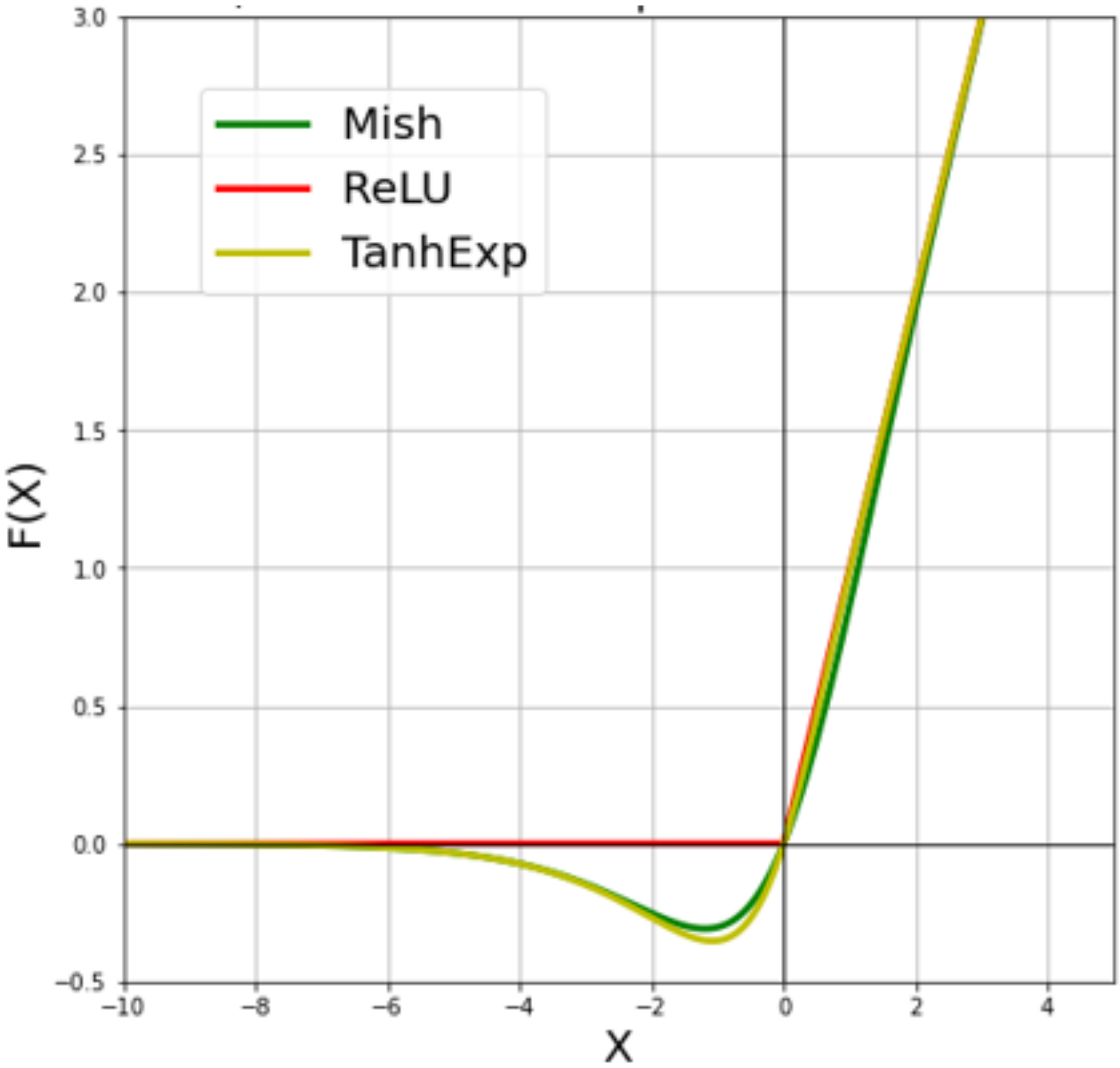Figure 2 depicts the activation functions used in this study, such as TanhExp, ReLU, and Mish. We chose ReLU because it is the standard function found in many CNN architectures, whereas TanhExp and Mish outperformed many other functions in the same category, including Swish and arctanh.

The nonlinearity of TanhExp and Mish makes their implementation on an embedded board a difficult task. To solve this issue, we need an approximation method to implement these functions on the FPGA. Numerous approximation methods have been applied to nonlinear functions in the state-of-the-art to facilitate their deployment on an embedded device. The authors of [12,18,33] implemented a nonlinear function on an FPGA using a polynomial approximation technique, such as the piecewise linear (PWL) approximation method or the quadratic approximation technique. These methods require the use of adders and multipliers. The look-up-table method was chosen by the authors in [34], which helped them to store the pre-calculated values. In addition, Reference [35] employs the coordinate rotation digital computer (CORDIC) technique.

Compared to other approximation methods, PWL requires fewer hardware resources and has significant precision. As a result, we chose the PWL approximation method to deploy the nonlinear Mish and TanhExp functions on an embedded device.

3.1.2. Pooling Layer

The pooling layer plays a role similar to that of the convolutional layer. It has to diminish the spatial size of the convolved feature. Furthermore, it aids in the reduction of feature dimensions while extracting the dominant characteristics to achieve a significant recognition rate. The well-known methods for performing pooling are average pooling and maximum pooling. Max-pooling aids in denoising the input while reducing the feature dimension. On the other hand, average pooling acts as a denoising mechanism for dimensionality reduction.

3.1.3. Fully-Connected Layer

The output of the convolution/pooling process was flattened and conducted into a single vector of values. Each value indicates the probability that the features and labels are similar. The fully connected layer is utilized to divulge the images into labels by using the features derived from the convolution/pooling process. Every neuron prioritizes the appropriate label for each received weight. After that, all neurons will ultimately vote about which label will win the classification.

3.2. Depthwise Separable Convolution

In recent years, many innovative network models, such as ShuffleNet and MobileNet, have been suggested to be deployed on an embedded board with limited memory and computing budgets. The main reason behind the success of these models is the use of the depthwise separable convolution (DSC) unit [36]. By reducing the number of parameters and network calculations, this unit demonstrated its effectiveness. However, a decrease in the number of parameters affected the precision of the network. Therefore, we considered the improvement of the DSC as a compromise between accuracy and cost. 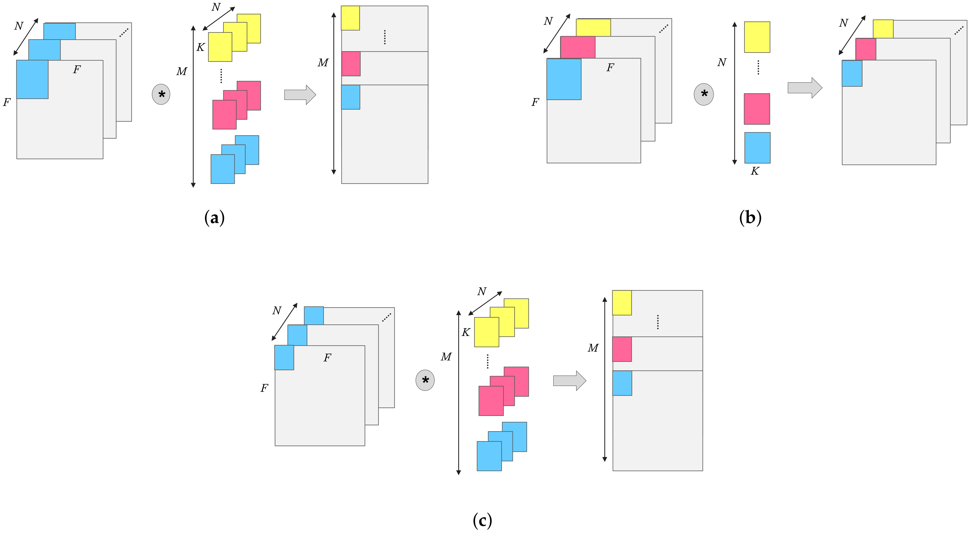Figure 3 depicts the standard convolution unit and depthwise separable convolution unit. For the standard convolution, the convolution results are summed to create one output channel for all the input channels that have been used by the convolution kernel. In contrast, the DSC is divided into a depthwise convolution (Dwcv) and a pointwise convolution (Pwcv). Dwcv uses a filter on each input channel to create the same number of outputs. Furthermore, Pwcv is a version of the standard convolution that uses a 1 × 1 filter.

Provided that the input feature map size is N × F × F, the filter size of the convolution is N × K × K × M, and the stride is 1. The number of parameters of the standard convolution layer is:

$$W_{Standardconvolution}=N\times M\times K\times K,$$

(2)

The number of calculations is:

$$O_{Standardconvolution}=N\times M\times K\times K\times F\times F,$$

(3)

The number of parameters of the DSC is:

$$W_{DSC}=N\times K\times K+N\times M,$$

(4)

The number of calculations of DSC is:

$$O_{DSC}=N\times K\times K\times F\times F+M\times N\times F\times F.$$

(5)

The main role of DSC is to reduce the number of parameters and network calculations. Therefore, the calculation of the reduction factors on weights is presented in Equation (6), while the reduction factor for operation is presented in Equation (7) as follows:

$$F_W=\frac{W_{DSC}}{W_{Standardconvolution}}=\frac{1}{K^2}+\frac{1}{M}.$$

(6)

$$F_O=\frac{O_{DSC}}{O_{Standardconvolution}}=\frac{1}{K^2}+\frac{1}{M}.$$

(7)

3.3. Arithmetic Representations

The selection of the arithmetic representation affects the performance of the CNN, such as the recognition rate, speed, energy dissipation, and hardware resources.

To achieve the desired results from the CNN implementation on the FPGA, we must select an appropriate arithmetic format. There are various formats to represent a real number in the state-of-the-art [37,38]. The integer fraction method for real number representation was introduced in [38]. The experimental results showed significant accuracy despite the use of a large number of hardware resources. The authors of [37] discussed the selection of an arithmetic number representation for network implementation on an FPGA. A comparison of precision and FPGA hardware resources for fixed-point and float-point representations was studied. The experimental results showed that a network with a fixed-point format used fewer hardware resources than a network with a float-point format. However, the network with float-point representation outperformed fixed-point representation in terms of accuracy. Almost every application that employs a CNN requires high precision and speed. As a result, we chose the float-point format for our FPGA implementation, which has acceptable precision. We then considered mitigating its disadvantage by improving our CNN model and reducing the number of calculations required.

4. Enhanced Architecture for Real-World Application: Ad-MobileNet Model

Nowadays, many tasks in computer vision are resolved using CNNs, such as image recognition. However, the use of the optimized version of CNNs in real-world applications is often demanded looking to their large number of parameters and calculations required for the network, as well as the limited memory on the embedded board. Hence, we considered developing a slim and thin model that provides high accuracy while utilizing a limited number of hardware resources. The proposed model is based on the shallow MobileNet-V1 model.

4.1. The Baseline MobileNet Model

The famous MobileNet-V1 [9] model is well-known for its small size, which was achieved using a DSC unit. This unit is constructed by a depthwise convolution (Dwcv) and a one-by-one pointwise convolution (Pwcv). The main idea of the DSC unit is to have different layers for combining and different layers for filtering. To further explain this, each input channel needs to be filtered separately in Dwcv, followed by Pwcv. In addition, the objective behind using Pwcv is to linearly combine all outputs of Dwcv. Generally, MobileNet uses the DSC unit to reduce the computation cost used on the network to approximately one-eighth of the standard convolutions.

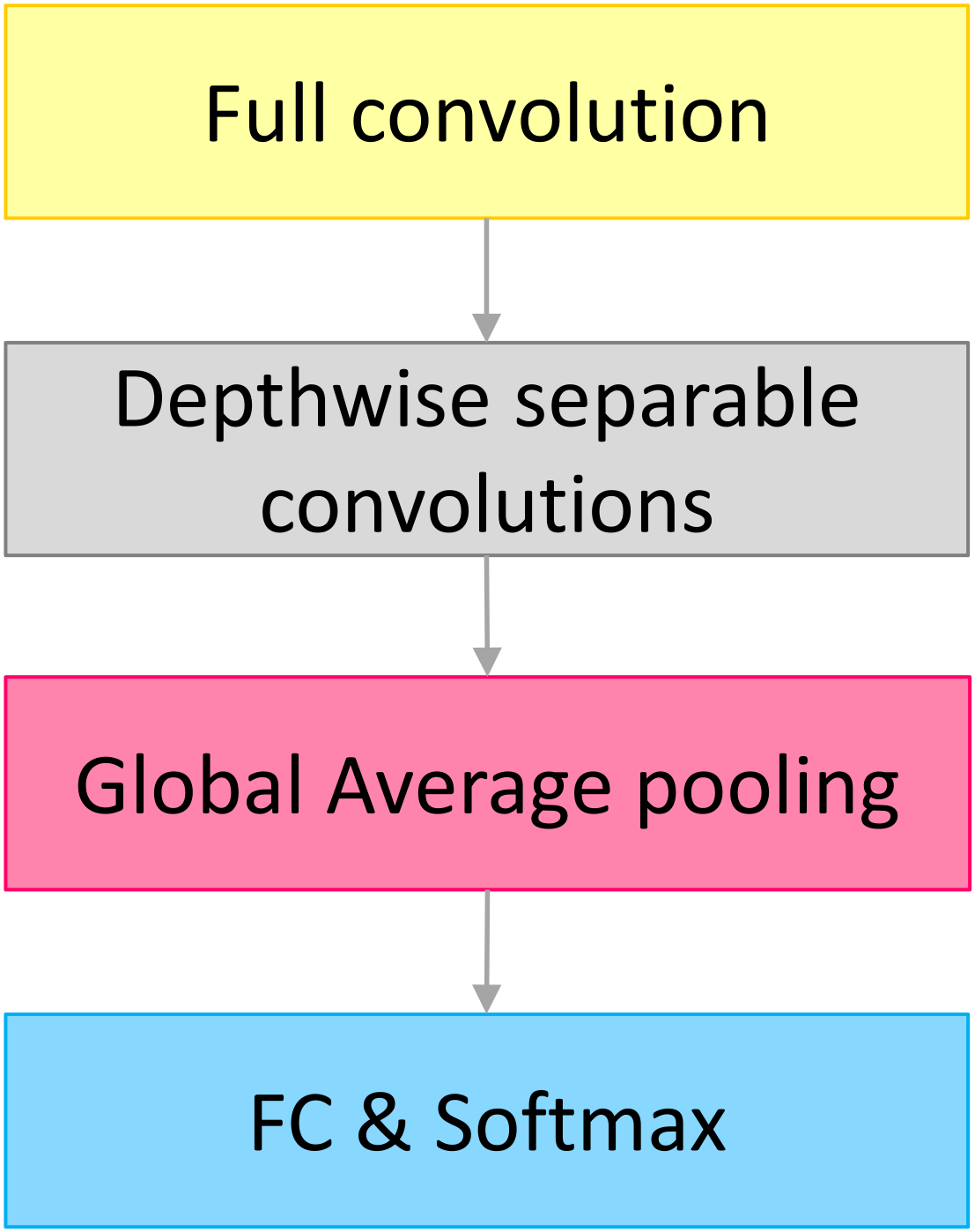
As shown in Figure 4, the baseline model is composed of a depthwise separable convolutions unit, full convolution layer, global average pooling layer, fully connected layer, and classification layer that uses the softmax function. Furthermore, the model has two hyperparameters, with values ranging from 0 to 1. These two hyperparameters are known as the width and resolution multipliers, and they can be used to shrink the model. However, using these two hyperparameters to reduce the size of the model always results in a significant decrease in the recognition rate.

4.2. The Proposed Model: Ad-MobileNet

We present our Ad-MobileNet model, which is based on the baseline MobileNet model. We made three types of modifications to the MobileNet-V1 model to achieve the Ad-MobileNet architecture. First, we replaced the DSC unit with the Ad-depth unit, which increased the accuracy. Second, we used various types of activation functions such as Mish, TanhExp, and ReLU, to enhance the overall accuracy of the model. Third, we removed all of the extraneous layers from the baseline model while altering the channel depth.

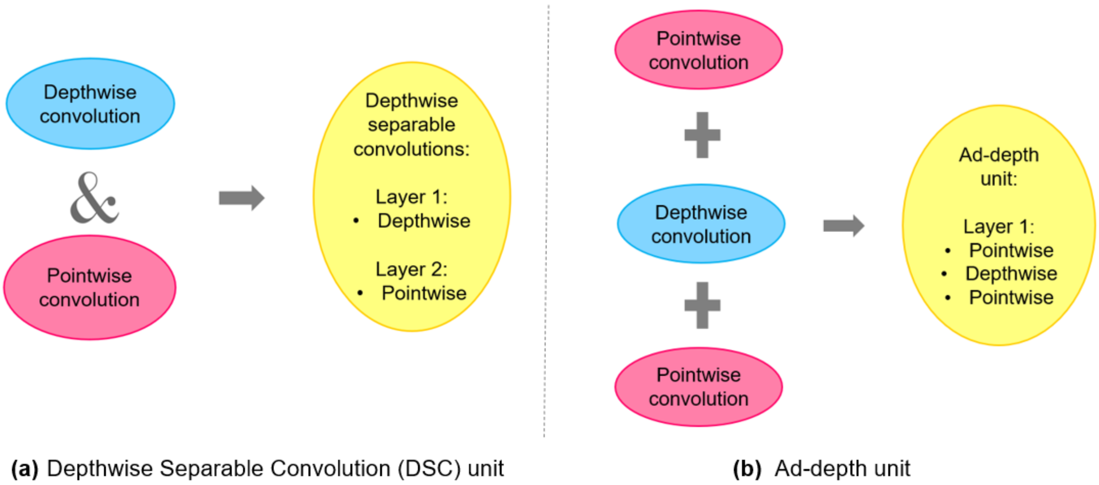
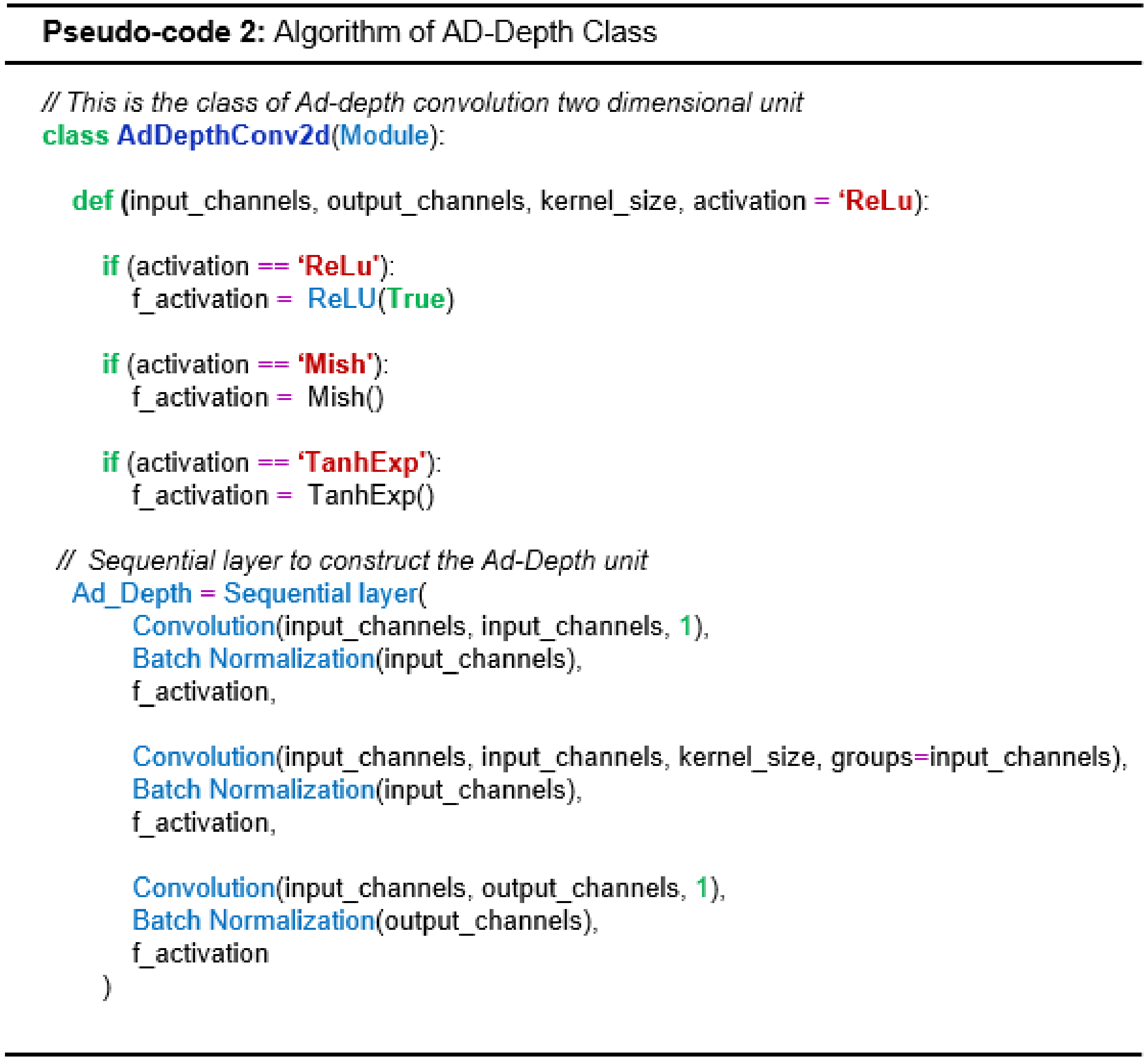
4.2.1. The First Modification: Using the Ad-Depth Unit

Each input channel in the DSC must be filtered separately in a Dwcv, followed by a Pwcv, where the outputs are linearly combined. In the baseline MobileNet model, Dwcv and Pwcv are defined separately. In our architecture, they are not defined as separate layers. Instead, we employed Ad-depth, which is made up of three combined layers. The Ad-depth is made up of two Pwcv on the edges and one Dwcv in the middle. They are combined into a single layer because there is no need to define them as separate layers. While the basic functionality of DSC remains unchanged, the number of layers is reduced to 14, which is half of the total number of layers in the MobileNet-V1 model, which has 28 layers. In summary, the Ad-depth unit was constructed of a single layer. This layer is formed by combining the Pwcv layer, the Dwcv layer, and another Pwcv layer. Figure 5 depicts the changes made to obtain the new unit Ad-depth used in the Ad-MobileNet model. This transformation improved the overall accuracy of the network.

4.2.2. The Second Modification: Using Enhanced Activation Functions Instead of ReLU

The activation function is important in the network because it determines whether or not to consider the neuron based on its value. Almost all modern architectures use the standard activation function ReLU. The ReLU activation function is extremely useful in almost every application. It does, however, have one fatal flaw, which is known as the dying ReLU. Even though this problem does not occur frequently, it can be fatal, particularly in real-time applications such as traffic sign recognition or medical image analysis applications that deal with human safety. TanhExp, Swish, and Mish are examples of enhanced functions that outperform the standard ReLU. As a result, we considered constructing three models, each of which uses a different activation function and comparing their performance to find the best-fit function that works well with our Ad-MobileNet model for image classification. TanhExp, ReLU, and Mish were chosen as activation functions. TanhExp and Mish are nonlinear functions with similar shapes. The TanhExp function is defined as

$$F\left(x\right)=x\times Tanh\left(exp\right(x\left)\right).$$

(8)

When x is greater than zero, TanhExp behaves roughly as the identity function, and when x is less than zero, it behaves roughly as the ReLU function. The Mish function is defined as follows:

$$F\left(x\right)=x\times Tanh\left(softplus\right(x\left)\right).$$

(9)

When x is greater than zero, Mish behaves roughly as the identity function, and when x is less than zero, it behaves roughly as the ReLU function. Mish and TanhExp appear similar, but they are not the same, and each has a unique impact on the network, such as in terms of accuracy or hardware resources. Figure 2 depicts the graphs of the TanhExp, ReLU, and Mish activation functions. The enhanced functions provide a boost in the overall accuracy of the Ad-MobileNet model.

4.2.3. The Third Modification: Dropping All the Unnecessary Layers

In this section, we attempt to reduce the calculation and number of parameters in the proposed model without sacrificing any necessary information. Hence, we considered removing repetitive and unnecessary layers. We drop the five layers from 9 to 13, which have the same output shape as (4,4,512). Furthermore, we discovered that reducing the channel depth of the last DSC unit from 1024 to 780 increased the recognition rate of the model by 1% while decreasing the number of computations simultaneously.

Table 1. Ad-MobileNet structure.

Layer	Output Shape	Stride
Input Layer	32,32,3	-
Basic convolution	32,32,32	s1
Depth separable conv	32,32,64	s1
Depth separable conv	16,16,128	s2
Depth separable conv	16,16,128	s1
Depth separable conv	8,8,256	s2
Depth separable conv	8,8,256	s1
Depth separable conv	4,4,512	s2
Depth separable conv	2,2,780	s2
Depth separable conv	2,2,780	s1
MaxPooling	1,1,780	s2
Global average pooling	1,1,780	s1
Fc + Softmax	1,1,10	s1

shows the various layers of the Ad-MobileNet model, the strides, and the output shape for each layer.

4.2.4. Ablation Study of the Ad-MobileNet Model’s Modifications

As previously stated, the primary objective of this article is to develop a model that maintains a balance between recognition rate and the number of parameters. To that end, we have listed three modifications that complement one another.

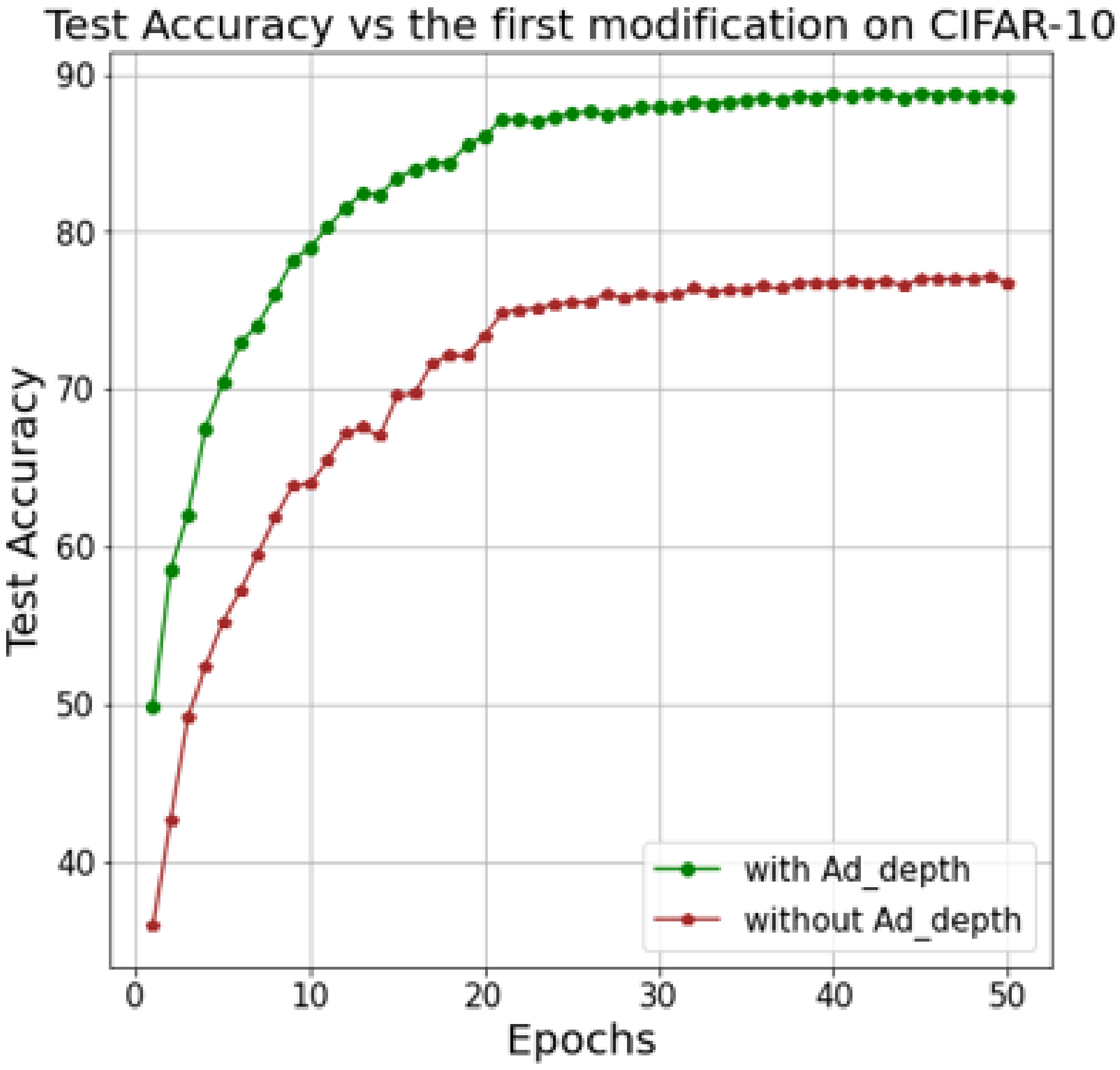
To determine the importance of the first modification, we compare the Ad-MobileNet with and without the Ad-depth unit while keeping the activation function as TanhExp (second modification) and removing all unnecessary layers from the baseline MobileNet (third modification). Figure 6 depicts the accuracy of Ad-MobileNet with and without the Ad-depth unit. Using the Ad-depth unit improves the model’s overall recognition rate, as shown in this figure. The Ad-depth, on the other hand, is composed of two Pwcv on the edges and one Dwcv in the middle, which reduces the number of parameters compared to the standard convolution but slightly increases the number of parameters compared to the DSC unit.

Provided that the input feature map size is N × F × F, the filter size of the convolution is N × K × K × M, and the stride is 1. The number of parameters of the standard convolution layer is presented in Equation (2), and the number of calculations is presented in Equation (3).

The number of parameters of the Ad-depth unit is:

$$W_{Addepth}=N\times K\times K+2\times N\times M,$$

(10)

The number of calculations of Ad-depth unit is:

$$O_{Addepth}=N\times K\times K\times F\times F+2\times M\times N\times F\times F.$$

(11)

The main role of the Ad-depth unit is to enhance the recognition rate while reducing the number of parameters and network calculations compared to the standard convolution. Therefore, the calculation of the reduction factors on weights is presented in Equation (12), while the reduction factor for operation is presented in Equation (13) as follows:

$$F_W=\frac{W_{Addepth}}{W_{Standardconvolution}}=\frac{2}{K^2}+\frac{1}{M}.$$

(12)

$$F_O=\frac{O_{Addepth}}{O_{Standardconvolution}}=\frac{2}{K^2}+\frac{1}{M}.$$

(13)

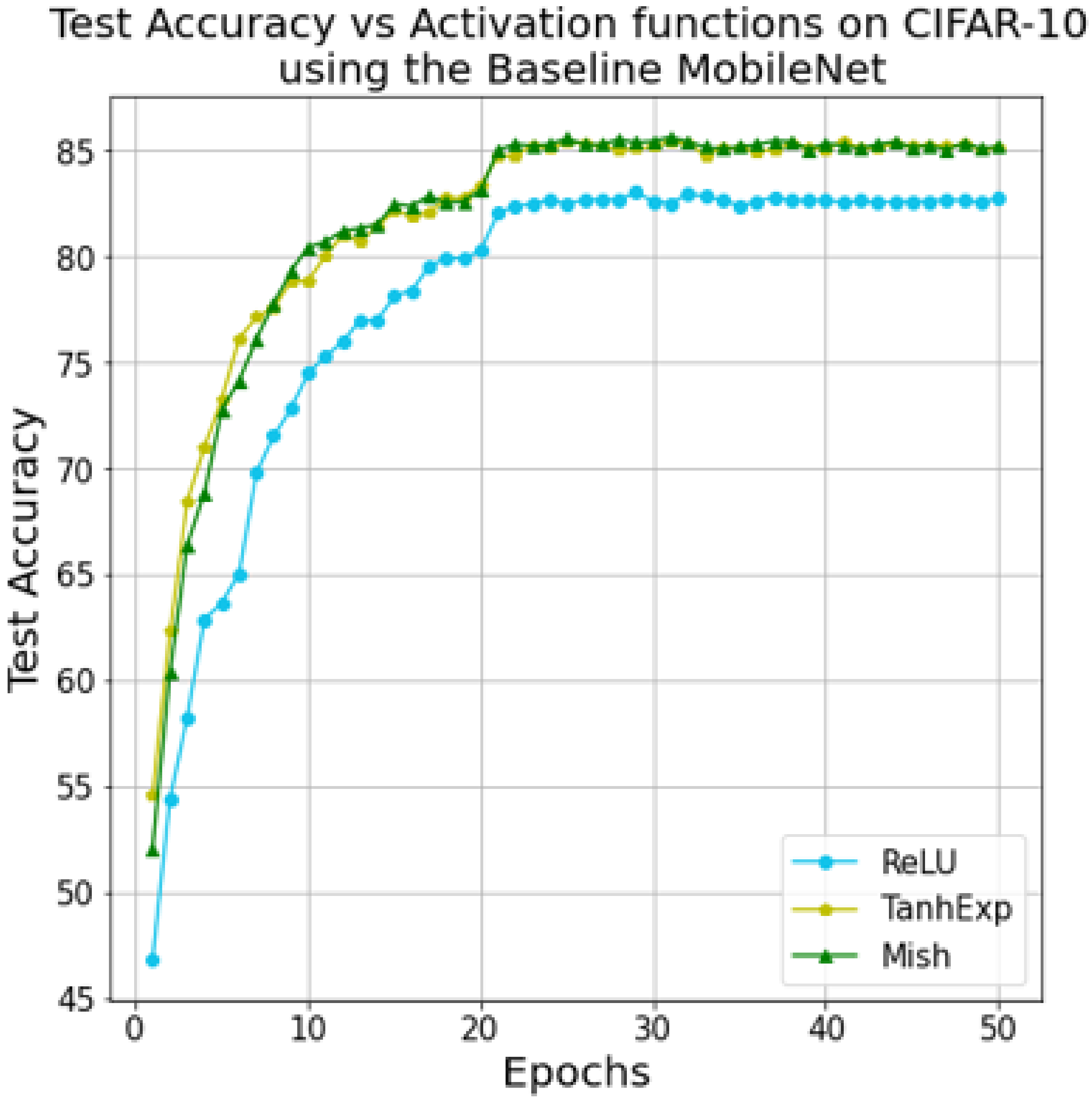
The second modification is to swap the activation function between Mish, TanhExp, and the standard ReLU. Figure 7 shows a comparison of test accuracy based on the baseline MobileNet when the activation function is changed. As illustrated in the graph, the model with TanhExp or Mish as the activation function outperforms the standard ReLU model. Various researches support this result in the literature [17,19,39,40].

The third modification is to remove any unnecessary layers. As shown in

Table 2. Ad-MobileNet with and without the third modification.

Model	Number of Parameters
Ad-MobileNet with 3rd modification	1,311,394
Ad-MobileNet without 3rd modification	3,238,058

, this modification has one flaw: it reduces the model’s performance while increasing its robustness. This is where the first and second modifications come into play; they ensure a balance between performance and robustness by masking the flaw of the third modification while retaining its advantage.

The ablation study may highlight the benefits and drawbacks of each modification and the benefit after using all three modifications, not just one. More specifically, each modification may cover the flaws of the other modification.

These modifications allow us to significantly reduced the computational number of the proposed model. Although the usage of the Ad-depth unit in place of the DSC unit slightly increases the computational number, we reduce more than 41% of the overall computations by removing the unnecessary layers and decreasing the channel depth of the last Ad-depth unit. A demonstration will be carried out in the experimental section. 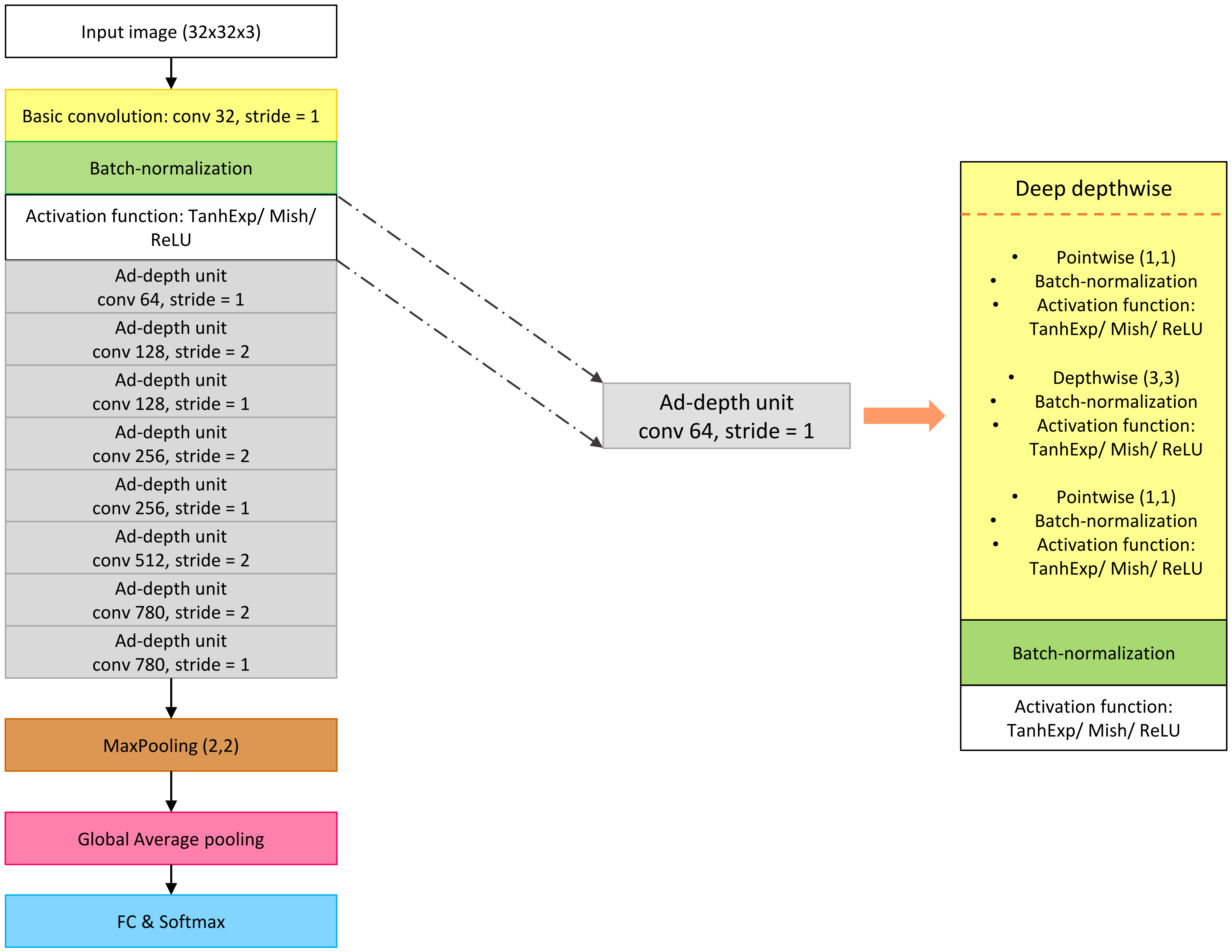Figure 8 depicts the architecture of the Ad-MobileNet model, which was obtained after implementing all of the modifications mentioned above.

5. Hardware Implementation of Ad-MobileNet on FPGA

To implement the Ad-MobileNet model on the FPGA, we elect the float-point representation to digitalize the real numbers, such as the weights, inputs, and biases. The float-point representation provides significant precision while requiring an acceptable number of hardware resources. Then, we need to arrange the implementation of the nonlinear activation functions for conducting the convolution layer and the Ad-depth unit on the FPGA.

5.1. Hardware Implementation of Activation Functions

We implemented three different activation functions. The first function was the standard ReLU. The implementation of this activation function, which is defined as follows: ReLU(X) = Max(X,0), is simple and depthless. This only requires registers (FF) and look-up tables (LUTs). However, the implementation of the two nonlinear activation functions, Mish (Equation (14)) and TanhExp (Equation (15)), is unique. They cannot be directly implemented on an FPGA. Hence, they require an approximation to be performed on an embedded board.

$$Mish\left(X\right)=X\times tanh\left(ln(1+e^X)\right)$$

(14)

$$TanhExp\left(X\right)=X\times tanh\left(e^X\right)$$

(15)

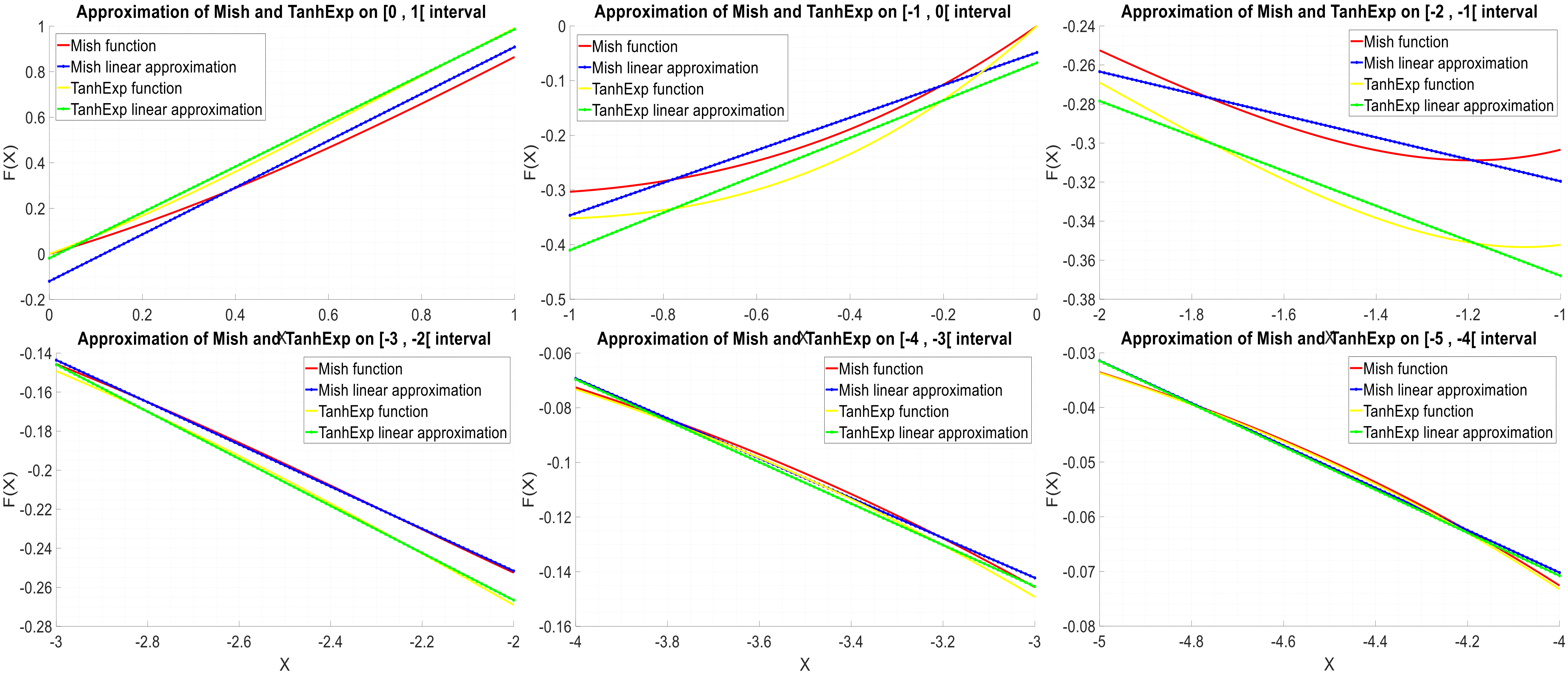
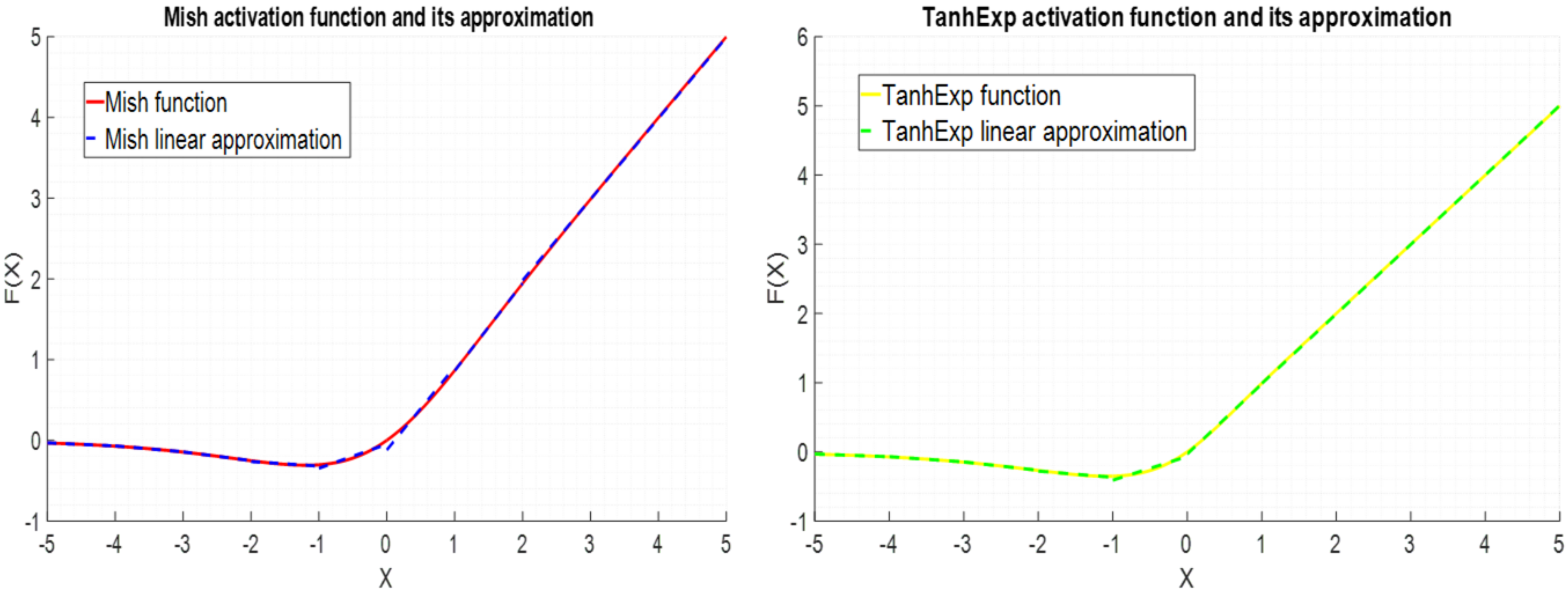
To implement the Ad-MobileNet model, we used the float-point format to perform the PWL approximation of the two nonlinear activation functions Mish and TanhExp. The PWL approximation of Mish (16) and that of TanhExp (17) are implemented on an embedded FPGA device using one adder, one multiplier, and registers for each approach function. The average and maximum errors of the PWL approximation of the Mish activation function are $\epsilon$${}_{avg}$ = 1.30 × 10${}^{-3}$ and $\epsilon$${}_{max}$ = 1.1989 × 10${}^{-1}$, respectively. On the other hand, the average and maximum errors of the PWL approximation of the TanhExp activation function are $\epsilon$${}_{avg}$ = 4.10524 × 10${}^{-4}$ and $\epsilon$${}_{max}$ = 6.743 × 10${}^{-2}$, respectively, which are lower than those of the Mish function. A comparison between the PWL approximations of Mish and TanhExp is shown in Figure 9. Figure 10 shows the graph of the activation functions and their approximations.

$$Mish\left(X\right)=\left\{\begin{array}{l}x,2<x\\ 1.08273\times x-0.22053,1<x\le 2\\ 1.02872\times x-0.11989,0<x\le 1\\ 0.29798\times x-0.04853,-1<x\le 0\\ -0.05617\times x-0.37574,-2<x\le -1\\ -0.10802\times x-0.46768,-3<x\le -2\\ -0.07294\times x-0.36108,-4<x\le -3\\ -0.03876\times x-0.22528,-5<x\le -4\\ -0.01855\times x-0.12508,-6<x\le -5\\ -0.00838\times x-0.06455,-7<x\le -6\\ -0.00049\times x-0.00632,x\le -7\end{array}\right\}$$

(16)

$$TanhExp\left(X\right)=\left\{\begin{array}{l}x,1<x\\ 1.00522\times x-0.01850,0<x\le 1\\ 0.34275\times x-0.06743,-1<x\le 0\\ -0.08953\times x-0.45752,-2<x\le -1\\ -0.12067\times x-0.50794,-3<x\le -2\\ -0.07575\times x-0.37267,-4<x\le -3\\ -0.03929\times x-0.22795,-5<x\le -4\\ -0.01864\times x-0.12562,-6<x\le -5\\ -0.00840\times x-0.06466,-7<x\le -6\\ -0.00049\times x-0.00632,x\le -7\end{array}\right\}$$

(17)

All of the requirements for implementing the nonlinear TanhExp and Mish activation functions using the PWL approach and float-point representation are now complete. As a result, we can implement a convolutional layer on an FPGA.

5.2. Hardware Implementation of Basic Convolutional Layer

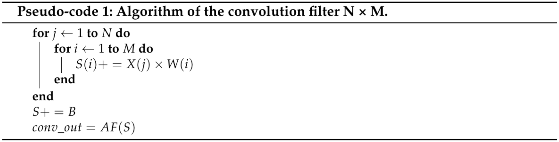
We decided to classify the images provided by the CIFAR-10 dataset as an application. This database uses two-dimensional data as input. Figure 11 depicts the hardware implementation of a convolution unit based on an N × M filter. The algorithm used for the convolution filter N × M is presented in Figure 12. This architecture takes advantage of the parallelism generated by the convolution layer to accelerate the application.

The convolutional layer employs the MACC mathematical operation. Therefore, we need to transfer the values of the inputs into a sliding window that has an identical weight filter size. The convolution operations are performed all at once, which assures the parallelization of the implementation. The accumulation of the weighted inputs constructs the main processing element (PE) in the convolution layer, as shown in Figure 11. Following the construction of the processing element, an adder was appended to add a bias to the nine values (for M × N = 3 × 3) acquired for each PE. Then, we apply an activation function to the output of that summation. In addition, the output of the activation functions is buffered and fed into the next layer. Figure 11 depicts how to build a convolution layer using a M × N filter. As previously stated, we intend to vary the activation function between the Mish, TanhExp, and ReLU. This step provides three CNN models, namely, MAd-MobileNet, TAd-MobileNet, and RAd-MobileNet.

5.3. Hardware Implementation of Ad-Depth Unit

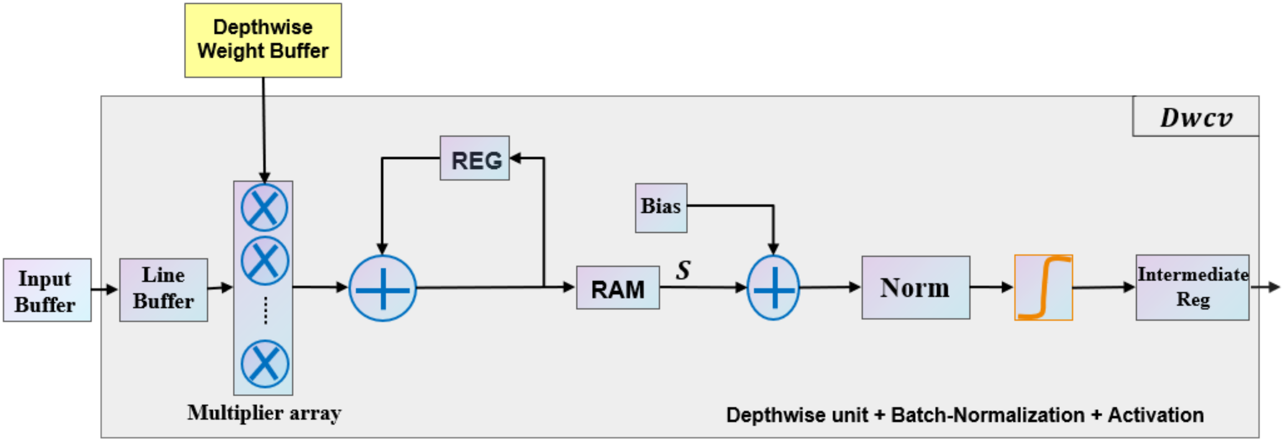
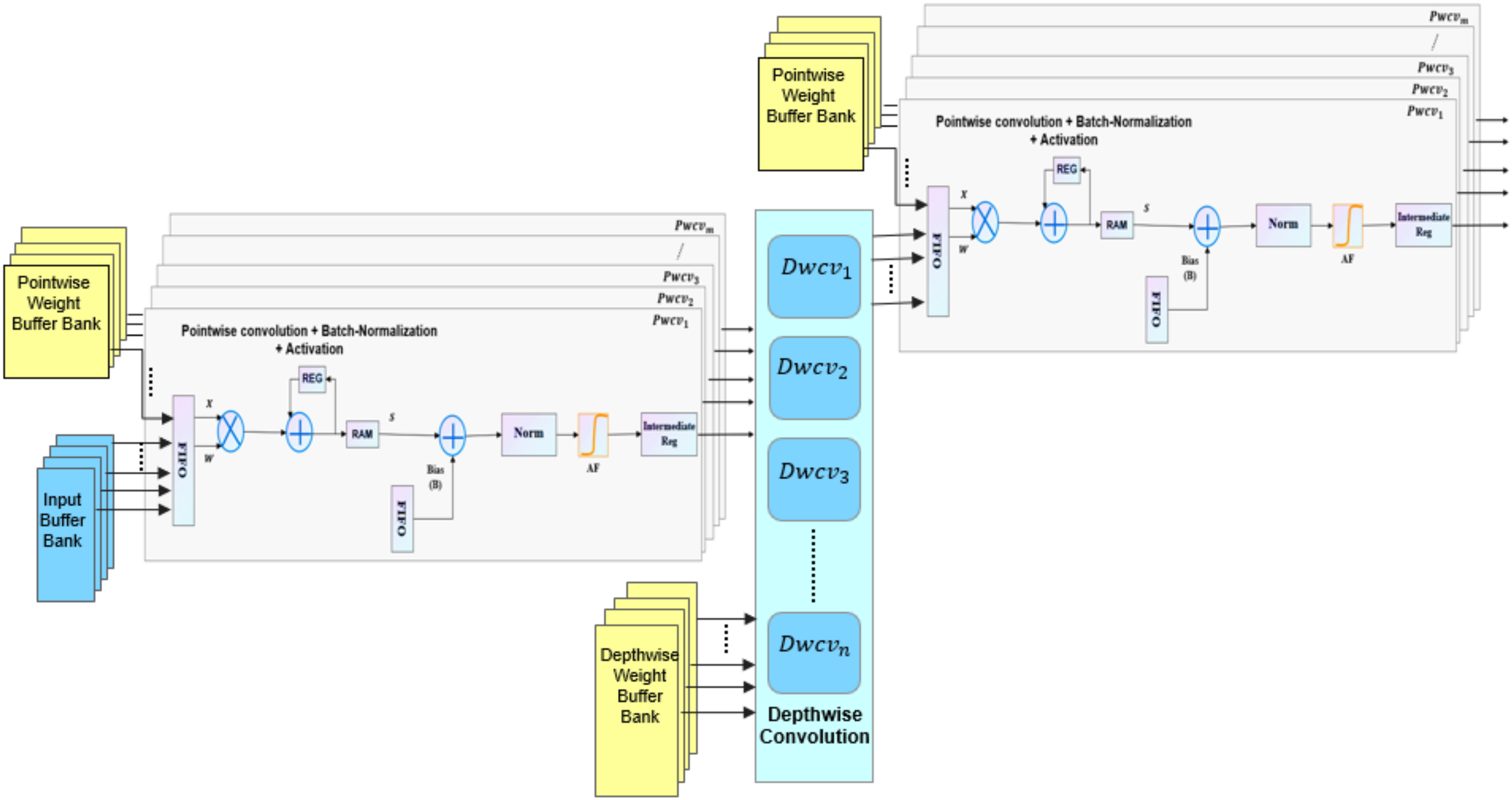
As mentioned in the previous sections, the Ad-depth unit is made up of two pointwise layers and one depthwise layer. In this study, the depthwise unit is composed of 32 slices of line buffer, 32 slices of multiplier array, adder, normalization block (Norm), and an activation block. Depthwise convolution is performed by k × k convolution operations with spatial proximity. When the input data are passed through the buffer in a row-major layout, sliding window selection is released by the line buffer on the input image. Furthermore, multiple rows of pixel values can be buffered for simultaneous access. As shown in Figure 13, each Dwcv unit manages the 2D convolutional operation of one input feature map and its corresponding weights. The construction of the Ad-depth unit is presented in Figure 14. Using multiple Dwcv units in parallel represents the depthwise convolution, which is depicted in Figure 15.

The pointwise convolution unit (Pwcv) is composed of a PE unit, adder, batch-normalization block (Norm), activation function module, ram, and registers, as shown in Figure 13. PE units operate a 1 × 1 convolution, which is accomplished by multiplying the depthwise convolution output by the pointwise weights, followed by the accumulation of all multipliers results. Then, a bias is added to the result of the multi-channels that are calculated using the adder and passed through the normalization block and activation module. We used a broadcast operation to copy the result of depthwise convolution to various Pwcv units, as depicted in Figure 15.

In the proposed model, we varied the activation function between the ReLU, TanhExp, and Mish functions to test their performance and influence over the Ad-MobileNet model. The experimental section presents the results of each implementation of the Ad-MobileNet model using these functions.

5.4. Hardware Implementation of Max-Pooling Layer

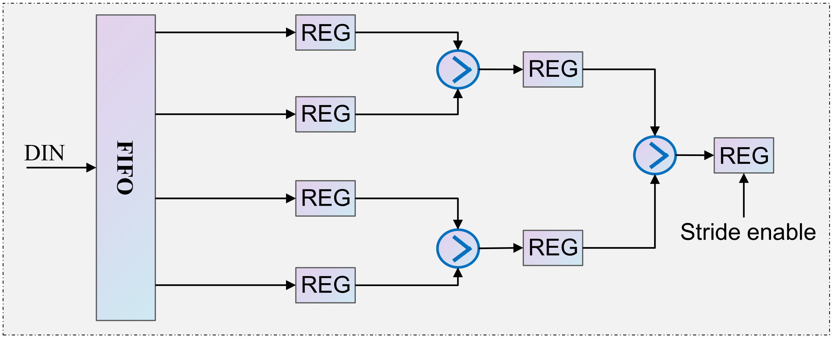
The pooling layer is the most basic unit of the CNN. In this layer, a sliding window is applied to all stored values obtained from the preceding layer. The pooling kernel reflects the sliding window size, whereas stride represents the step size. Then, we elect the average or maximum value in the sliding window, which is based on the type of pool chosen. Figure 16 shows a sample of the hardware architecture corresponding to the max-pooling layer. We used a 2 × 2 pooling filter and a stride of size “2”. Each pair of values in the sliding window is compared to determine which is greater.

The Ad-MobileNet module uses the global average pooling (GAP) instead of the fully connected layer, which is simple to conduct on FPGA and requires fewer parameters compared to the fully connected layer. GAP is similar to the pooling layer in that we need to find the mean output of each feature map in the previous layer while using a pool size equal to the input.

6. Experiment and Results

We implemented the models MAd-MobileNet, TAd-MobileNet, and RAd-MobileNet, which use the activation functions Mish, TanhExp, and ReLU successively on FPGA xc7vx980t of the Virtex-7 family. To demonstrate the functionality of these models, we used an image classification application, which is based on the CIFAR-10 dataset. This database contains ten classes. To carry out this experiment, we used VHDL as the hardware definition language.

After implementing the modifications described in Section 4, the Ad-MobileNet architecture was obtained. We varied the activation function between ReLU, Mish, and TanhExp activation functions using the PWL approach method to represent nonlinear functions. We erased the five needless layers while changing the channel depth in the last DSC unit from 1024 to 780. We replaced the DSC unit with a thicker one, which is named the Ad-depth unit. The Ad-depth unit combines the Pwcv, Dwcv, and Pwcv layers into a single deep layer. These modifications help to improve the recognition rate of the Ad-MobileNet network while minimizing the number of hardware resources. 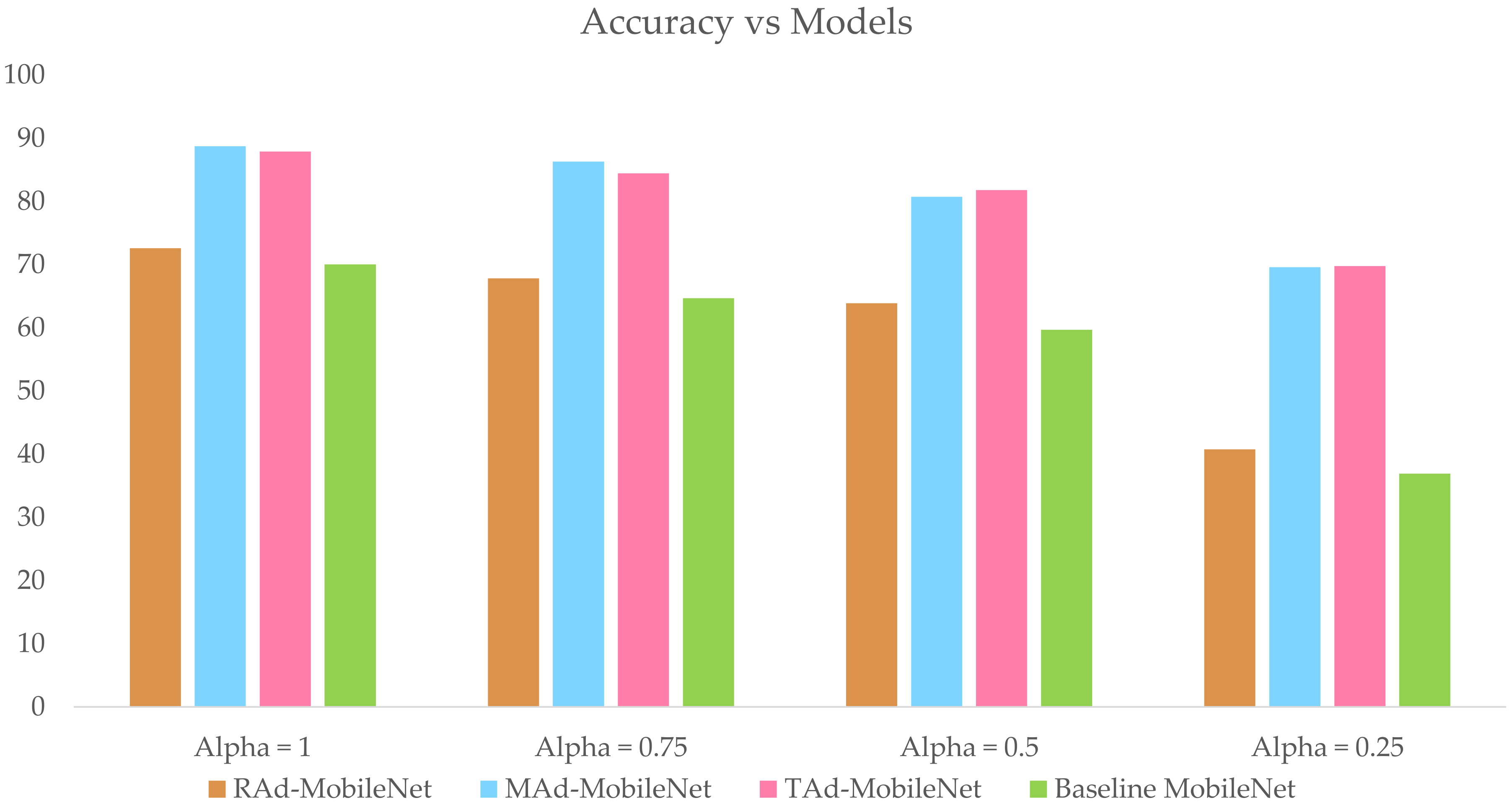Figure 17 illustrates the comparison of the top-1 test accuracy between the baseline MobileNet, RAd-MobileNet, TAd-MobileNet, and MAd-MobileNet models while varying the width multiplier (alpha) using the CIFAR-10 dataset.

Figure 17 proves that the baseline MobileNet model has the lowest accuracy. Furthermore, MAd-MobileNet and TAd-MobileNet outperform the two other models in terms of recognition rate achieving 88.76% and 87.88%, respectively. However, the RAd-MobileNet has the lowest number of hardware resources. It reduces more than 41% of the DSP used compared to that used in the implementation of the baseline MobileNet, which is illustrated in

Table 3. Hardware resources of Ad-MobileNet model on varying the activation function.

Model	DSP	LUTs	FF
Baseline MobileNet	1593	137,291	183,614
RAd-MobileNet	937	57,438	79,327
MAd-MobileNet	1128	68,796	87,569
TAd-MobileNet	1128	69,163	86,251

. In addition, Table 3 proves that implementing the Network using an advanced nonlinear activation function on FPGA slightly increases the number of hardware resources compared to that using ReLU.

As shown in Figure 17 and

Table 4. Performance of Ad-MobileNet model using ReLU activation function on varying alpha.

Model	Model Size (MB)	Parameters	Frequency (MHz)
Baseline MobileNet ($\alpha$ = 1)	38.2	3,223,178	110
Ad-MobileNet ($\alpha$ = 1)	5.11	1,311,394	225
Ad-MobileNet ($\alpha$ = 0.75)	2.94	746,593	245
Ad-MobileNet ($\alpha$ = 0.5)	1.38	339,762	270
Ad-MobileNet ($\alpha$ = 0.25)	0.42	90,901	310

, the width multiplier has a significant influence on the recognition rate and size of the model. Hence, we can say that increasing alpha increases the accuracy and number of hardware resources. For alpha equal to 1, RAd-MobileNet has a 2.57% higher recognition rate than the baseline MobileNet architecture, TAd-MobileNet has a 17.05% higher recognition rate, and MAd-MobileNet has an 18.72% higher recognition rate. Ad-Mobile Nets (alpha = 0.25), on the other hand, outperforms the other architectures in terms of model size, frequency, and number of parameters. When we changed the alpha to 0.25, we reduced the number of parameters by 97.17%.

There is no such thing as a perfect network, but there is such a thing as a well-fitting network. As a result, we have the flexibility to select any model that meets our requirements. For example, if we need an ultra-thin model with adequate accuracy, we can use any one of the Ad-MobileNet models with a width multiplier equal to 0.5. If we need a higher precision in the classification, we can use the MAd-MobileNet network with a width multiplier equal to 1.

7. Discussion

7.1. Comparison with MobileNet-V1 Model

In this section, we compare our networks to the MobileNet model to ensure that the suggested architectures are both efficient in terms of the recognition rate and suitable in terms of hardware resources for real-world applications.

Table 5. Performance comparison of the baseline MobileNet and the Ad-MobileNet models on FPGA.

Model	Baseline MobileNet	RAd-MobileNet	MAd-MobileNet	TAd-MobileNet
FPGA	Virtex-7 xc7vx980	Virtex-7 xc7vx980	Virtex-7 xc7vx980	Virtex-7 xc7vx980
Top-1 test accuracy (%)	70.04	72.61	88.76	87.09
Frequency (MHz)	160	225	200	205
DSP	1842	937	1128	1128
LUT	127,325	57,438	68,796	69,163
FF	183,211	79,327	87,569	86,251

compares the performance of the baseline MobileNet and our networks implemented on an FPGA using the same CIFAR-10 database.

In this section, we present an analysis comparing the efficiency and performance of hardware implementation of our proposed models to baseline MobileNet architecture. Table 5 shows the performance comparison of MobileNets hardware implementations on FPGA. Based on the speed and computation of hardware resources, we compared the effectiveness of our algorithms to the baseline MobileNet model used on the same board. The baseline MobileNet model achieved the worst accuracy, speed, and the highest number of hardware resources in the table. For more detail, we compared the standard MobileNet to the Ad-MobileNet networks. MAd-MobileNet is an Ad-MobileNet model that uses Mish as its activation function. This model achieved an accuracy of 88.76%, which is the highest in Table 5 and higher than the baseline MobileNet model by 18.72%. Furthermore, the MAd-MobileNet model achieved a speed of 200 MHz, which is higher than that of the baseline model by 40 MHz. Even for the hardware resources, MAd-MobileNet used 38.7% DSP less than that used in the implementation of the standard MobileNet. RAd-MobileNet is an Ad-MobileNet model that uses ReLU as its activation function. This model achieved an accuracy of 72.61%, which is higher than that of the standard MobileNet only by 2.6%. However, the RAd-MobileNet model achieved a speed of 225 MHz, which is the highest in the table and higher than that of the baseline model by 65 MHz. Furthermore, the number of hardware resources used in the implementation of RAd-MobileNet is the lowest in the table and lower by 50% than that used in the standard MobileNet.

MAd-MobileNet and TAd-MobileNet architectures consecutively used the activation functions Mish and TanhExp. They both used slightly more hardware resources than RAd-MobileNet, which used ReLU as its activation function. The comparison in Table 5 shows that our models surpass MobileNet-V1 model in terms of speed and accuracy (Figure 17) while using fewer hardware resources.

7.2. Comparison with the State-of-the-Art

In this section, we compare our networks to existing ones in the literature to ensure that the suggested architectures are both efficient in terms of the recognition rate and suitable in terms of hardware resources for real-world applications.

Table 6. Performance comparison with other MobileNet models on FPGA.

Model	[41]	[22]	[42]	[21]	RAd-MobileNet
FPGA	Intel Stratix 10	XCZU19EG	XCZU9EG	ZYNQ 7100	Virtex-7 xc7vx980
Frequency (MHz)	156	200	150	100	225
DSP	297	1020	1452	1926	937
LUT	926,000	368,936	139,000	142,291	57,438
FF	583,000	391,517	55,000	187,146	79,327
Power (W)	-	7.35	-	4.083	3.25

compares the performance of the networks implemented on an FPGA using the same CIFAR-10 database.

In this section, we present an analysis comparing the efficiency and performance of hardware implementation of our proposed models to existing MobileNet-based architectures in the literature. Table 6 illustrates the performance comparison of various hardware implementations on the FPGA. Based on the speed and computation of hardware resources, we compared the effectiveness of various algorithms used on FPGAs. The authors of [21] proposed a CNN accelerator based on the MobileNet structure that can accelerate both standard and depthwise separable convolutions. They used ReLU as the activation function. They achieved a speed of 100 MHz, which is the slowest in Table 6 and slower than our suggested RAd-MobileNet model by 125 MHz. Furthermore, their model necessitated a large number of hardware resources of 1926 DSP, which is the highest in the table. They used 989 DSP more than that used in the implementation of RAd-MobileNet. In addition, they used a power consumption higher by 0.8 W more than that of RAd-MobileNet. The authors of [42] adopted an implementation of the RRMobileNet model using two levels of redundancy data-level and model-level redundancy. Their suggestion achieved a frequency of 150 MHz, which is the second-lowest frequency in the table. In addition, they used a large computational hardware resource of 1452 DSP, which is the second-highest in the table. Furthermore, they drew on a significant amount of logic element 139 K (LUT), which is more than double the amount used in our proposed models. The authors of [41] proposed Tomato, a framework designed to automate the process of generating efficient CNN accelerators. The implementation of MobileNet-V1 based on their suggestion achieved the fewest hardware resources in terms of DSP. However, they used the highest number of LUTs and FFs in the table. They used more than 16× as many LUTs as we did in our implementations. Furthermore, the speed of their model was 69 MHz slower than that of our model. The authors of [22] proposed an accelerator for inference on the MobileNet-V2 network using a heterogeneous system. Their system achieved a significant speed of 200 MHz, which is the second-highest speed of our RAd-MobileNet model. However, they used 83 DSP more than that used in the RAd-MobileNet implementation. Furthermore, they used more than 6× as many LUTs, as we did in our implementations. They also used a power of 7.35 W, which is higher than that of RAd-MobileNet by 4.1 W.

The comparison in Table 6 shows that our models achieve competitive results in terms of speed, power consumption and accuracy (Figure 17) while using fewer hardware resources. To summarize, we can select the model that best meets our requirements in terms of computational hardware resources, speed, or accuracy.

8. Conclusions

In this study, we intended to build a network with a few hardware resources while providing a high classification rate without losing information and implementing it on an FPGA. We improved the MobileNet-V1 architecture to achieve this goal. We changed the three aspects of the original design. First, we removed the needless layers that had the same output shape as (4,4,512). Second, we varied the activation functions of Mish, TanhExp, and ReLU. The activation functions Mish, TanhExp, and ReLU were used in the models MAd-MobileNet, TAd-MobileNet, and RAd-MobileNet, respectively. Both nonlinear activation functions Mish and TanhExp were implemented on an FPGA using PWL approximation. Furthermore, to digitalize real numbers, we adopted a float-point format. Third, we replaced the depth-separable convolution unit with a thicker one, named the Ad-depth unit, which enhances the recognition rate of the model. We compared the number of hardware resources, power consumption, speed, and accuracy required for FPGA implementation on the Virtex-7 board. We achieved an 88.76% recognition rate with the MAd-MobileNet model, which is 18.72% higher than the baseline MobileNet model. Furthermore, we achieved a speed of 225 MHz using the RAd-MobileNet network, which is more than 120 MHz faster than the baseline model.

It is worth noting that the previously discussed results were obtained using a simple database CIFAR-10 for an image classification application. As a result, we decided to study the Ad-MobileNet model using larger databases and different applications in order to discover each flaw and advantage as part of our future work.

References

- Zagoruyko, S.; Komodakis, N. Wide Residual Networks. In Proceedings of the British Machine Vision Conference 2016, York, UK, 19–22 September 2016; pp. 1–87. [Google Scholar] [CrossRef] [Green Version]
- Szegedy, C.; Liu, W.; Jia, Y.; Sermanet, P.; Reed, S.; Anguelov, D.; Erhan, D.; Vanhoucke, V.; Rabinovich, A. Going deeper with convolutions. In Proceedings of the 2015 IEEE Conference on Computer Vision and Pattern Recognition (CVPR), Boston, MA, USA, 7–12 June 2015; pp. 1–9. [Google Scholar] [CrossRef] [Green Version]
- Iandola, F.N.; Han, S.; Moskewicz, M.W.; Ashraf, K.; Dally, W.J.; Keutzer, K. SqueezeNet: AlexNet-level accuracy with 50x fewer parameters and <0.5 MB model size. arXiv 2016, arXiv:1602.07360. [Google Scholar]
- Huang, G.; Liu, Z.; Van Der Maaten, L.; Weinberger, K.Q. Densely Connected Convolutional Networks. In Proceedings of the 2017 IEEE Conference on Computer Vision and Pattern Recognition (CVPR), Honolulu, HI, USA, 21–26 July 2017; pp. 2261–2269. [Google Scholar] [CrossRef] [Green Version]
- He, K.; Zhang, X.; Ren, S.; Sun, J. Deep Residual Learning for Image Recognition. In Proceedings of the 2016 IEEE Conference on Computer Vision and Pattern Recognition (CVPR), Las Vegas, NV, USA, 27–30 June 2016; pp. 770–778. [Google Scholar] [CrossRef] [Green Version]
- Alom, M.Z.; Taha, T.M.; Yakopcic, C.; Westberg, S.; Sidike, P.; Nasrin, M.S.; Van Esesn, B.C.; Awwal, A.A.S.; Asari, V.K. The History Began from AlexNet: A Comprehensive Survey on Deep Learning Approaches. arXiv 2018, arXiv:1803.01164. [Google Scholar]
- Ben Fredj, H.; Bouguezzi, S.; Souani, C. Face recognition in unconstrained environment with CNN. Vis. Comput. 2021, 37, 217–226. [Google Scholar] [CrossRef]
- Belabed, T.; Coutinho, M.G.F.; Fernandes, M.A.C.; Sakuyama, C.V.; Souani, C. User Driven FPGA-Based Design Automated Framework of Deep Neural Networks for Low-Power Low-Cost Edge Computing. IEEE Access 2021, 9, 89162–89180. [Google Scholar] [CrossRef]
- Howard, A.G.; Zhu, M.; Chen, B.; Kalenichenko, D.; Wang, W.; Weyand, T.; Andreetto, M.; Adam, H. MobileNets: Efficient Convolutional Neural Networks for Mobile Vision Applications. arXiv 2017, arXiv:1704.04861. [Google Scholar]
- Bouguezzi, S.; Faiedh, H.; Souani, C. Slim MobileNet: An Enhanced Deep Convolutional Neural Network. In Proceedings of the 2021 18th International Multi-Conference on Systems, Signals & Devices (SSD), Monastir, Tunisia, 22–25 March 2021; pp. 12–16. [Google Scholar] [CrossRef]
- Zhang, X.; Zhou, X.; Lin, M.; Sun, J. ShuffleNet: An Extremely Efficient Convolutional Neural Network for Mobile Devices. In Proceedings of the 2018 IEEE/CVF Conference on Computer Vision and Pattern Recognition, Salt Lake City, UT, USA, 18–23 June 2018; pp. 6848–6856. [Google Scholar] [CrossRef] [Green Version]
- Tsmots, I.; Skorokhoda, O.; Rabyk, V. Hardware Implementation of Sigmoid Activation Functions using FPGA. In Proceedings of the 2019 IEEE 15th International Conference on the Experience of Designing and Application of CAD Systems (CADSM), Polyana, Ukraine, 26 February–2 March 2019; pp. 34–38. [Google Scholar] [CrossRef]
- Pan, S.P.; Li, Z.; Huang, Y.J.; Lin, W.C. FPGA realization of activation function for neural network. In Proceedings of the 2018 7th International Symposium on Next Generation Electronics (ISNE), Taipei, Taiwan, 7–9 May 2018; pp. 1–2. [Google Scholar] [CrossRef]
- Nair, V.; Hinton, G.E. Rectified linear units improve Restricted Boltzmann machines. In Proceedings of the ICML 2010-Proceedings, 27th International Conference on Machine Learning, Haifa, Israel, 21–24 June 2010. [Google Scholar] [CrossRef]
- Xie, Y.; Joseph Raj, A.N.; Hu, Z.; Huang, S.; Fan, Z.; Joler, M. A Twofold Lookup Table Architecture for Efficient Approximation of Activation Functions. IEEE Trans. Very Large Scale Integr. (VLSI) Syst. 2020, 28, 2540–2550. [Google Scholar] [CrossRef]
- Givaki, K.; Salami, B.; Hojabr, R.; Reza Tayaranian, S.M.; Khonsari, A.; Rahmati, D.; Gorgin, S.; Cristal, A.; Unsal, O.S. On the Resilience of Deep Learning for Reduced-voltage FPGAs. In Proceedings of the 2020 28th Euromicro International Conference on Parallel, Distributed and Network-Based Processing (PDP), Västerås, Sweden, 11–13 March 2020; pp. 110–117. [Google Scholar] [CrossRef]
- Liu, X.; Di, X. TanhExp: A smooth activation function with high convergence speed for lightweight neural networks. IET Comput. Vis. 2021, 15, 136–150. [Google Scholar] [CrossRef]
- Bouguezzi, S.; Faiedh, H.; Souani, C. Hardware Implementation of Tanh Exponential Activation Function using FPGA. In Proceedings of the 2021 18th International Multi-Conference on Systems, Signals & Devices (SSD), Monastir, Tunisia, 22–25 March 2021; pp. 1020–1025. [Google Scholar] [CrossRef]
- Misra, D. Mish: A Self Regularized Non-Monotonic Activation Function. arXiv 2019, arXiv:1908.08681. [Google Scholar]
- Li, Z.-l.; Wang, L.-y.; Yu, J.-y.; Cheng, B.-w.; Hao, L. The Design of Lightweight and Multi Parallel CNN Accelerator Based on FPGA. In Proceedings of the 2019 IEEE 8th Joint International Information Technology and Artificial Intelligence Conference (ITAIC), Chongqing, China, 24–26 May 2019; pp. 1521–1528. [Google Scholar] [CrossRef]
- Liu, B.; Zou, D.; Feng, L.; Feng, S.; Fu, P.; Li, J. An FPGA-Based CNN Accelerator Integrating Depthwise Separable Convolution. Electronics 2019, 8, 281. [Google Scholar] [CrossRef] [Green Version]
- Pérez, I.; Figueroa, M. A Heterogeneous Hardware Accelerator for Image Classification in Embedded Systems. Sensors 2021, 21, 2637. [Google Scholar] [CrossRef] [PubMed]
- Farrukh, F.U.D.; Xie, T.; Zhang, C.; Wang, Z. Optimization for Efficient Hardware Implementation of CNN on FPGA. In Proceedings of the 2018 IEEE International Conference on Integrated Circuits, Technologies and Applications (ICTA), Beijing, China, 21–23 November 2018; pp. 88–89. [Google Scholar] [CrossRef]
- Chang, X.; Pan, H.; Zhang, D.; Sun, Q.; Lin, W. A Memory-Optimized and Energy-Efficient CNN Acceleration Architecture Based on FPGA. In Proceedings of the 2019 IEEE 28th International Symposium on Industrial Electronics (ISIE), Vancouver, BC, Canada, 12–14 June 2019; pp. 2137–2141. [Google Scholar] [CrossRef]
- Huang, C.; Ni, S.; Chen, G. A layer-based structured design of CNN on FPGA. In Proceedings of the 2017 IEEE 12th International Conference on ASIC (ASICON), Guiyang, China, 25–28 October 2017; pp. 1037–1040. [Google Scholar] [CrossRef]
- Hailesellasie, M.; Hasan, S.R.; Khalid, F.; Awwad, F.; Shafique, M. FPGA-Based Convolutional Neural Network Architecture with Reduced Parameter Requirements. In Proceedings of the IEEE International Symposium on Circuits and Systems, Florence, Italy, 27–30 May 2018. [Google Scholar] [CrossRef]
- Wu, D.; Zhang, Y.; Jia, X.; Tian, L.; Li, T.; Sui, L.; Xie, D.; Shan, Y. A High-Performance CNN Processor Based on FPGA for MobileNets. In Proceedings of the 2019 29th International Conference on Field Programmable Logic and Applications (FPL), Barcelona, Spain, 8–12 September 2019; pp. 136–143. [Google Scholar] [CrossRef]
- Liang, Y.; Lu, L.; Xiao, Q.; Yan, S. Evaluating fast algorithms for convolutional neural networks on FPGAs. IEEE Trans. Comput.-Aided Des. Integr. Circuits Syst. 2020, 39, 857–870. [Google Scholar] [CrossRef]
- Simonyan, K.; Zisserman, A. Very deep convolutional networks for large-scale image recognition Karen. arXiv 2014, arXiv:1409.1556. [Google Scholar]
- Xie, S.; Girshick, R.; Dollar, P.; Tu, Z.; He, K. Aggregated Residual Transformations for Deep Neural Networks. In Proceedings of the 2017 IEEE Conference on Computer Vision and Pattern Recognition (CVPR), Honolulu, HI, USA, 21–26 July 2017; pp. 5987–5995. [Google Scholar] [CrossRef] [Green Version]
- Bouguezzi, S.; Ben Fredj, H.; Faiedh, H.; Souani, C. Improved architecture for traffic sign recognition using a self-regularized activation function: SigmaH. Vis. Comput. 2021, 1–18. [Google Scholar] [CrossRef]
- Ramachandran, P.; Zoph, B.; Le, Q.V. Swish a self-gated activation function. arXiv 2017, arXiv:1710.05941. [Google Scholar]
- Yesil, S.; Sen, C.; Yilmaz, A.O. Experimental Analysis and FPGA Implementation of the Real Valued Time Delay Neural Network Based Digital Predistortion. In Proceedings of the 2019 26th IEEE International Conference on Electronics, Circuits and Systems (ICECS), Genoa, Italy, 27–29 November 2019; pp. 614–617. [Google Scholar] [CrossRef]
- Piazza, F.; Uncini, A.; Zenobi, M. Neural networks with digital LUT activation functions. In Proceedings of the 1993 International Conference on Neural Networks (IJCNN-93-Nagoya, Japan), Nagoya, Japan, 25–29 October 1993; Volume 2, pp. 1401–1404. [Google Scholar] [CrossRef]
- Tiwari, V.; Khare, N. Hardware implementation of neural network with Sigmoidal activation functions using CORDIC. Microprocess. Microsyst. 2015, 39, 373–381. [Google Scholar] [CrossRef]
- Chollet, F. Xception: Deep Learning with Depthwise Separable Convolutions. In Proceedings of the 2017 IEEE Conference on Computer Vision and Pattern Recognition (CVPR), Honolulu, HI, USA, 21–26 July 2017; pp. 1800–1807. [Google Scholar] [CrossRef] [Green Version]
- Savich, A.; Moussa, M.; Areibi, S. A scalable pipelined architecture for real-time computation of MLP-BP neural networks. Microprocess. Microsyst. 2012, 36, 138–150. [Google Scholar] [CrossRef]
- Nedjah, N.; da Silva, R.M.; de Macedo Mourelle, L. Compact yet efficient hardware implementation of artificial neural networks with customized topology. Expert Syst. Appl. 2012, 39, 9191–9206. [Google Scholar] [CrossRef]
- Marina Adriana Mercioni, S.H. Novel Activation Functions Based on TanhExp Activation Function in Deep Learning. Int. J. Future Gener. Commun. Netw. 2020, 13, 2415–2426. [Google Scholar]
- Zhang, Z.; Yang, Z.; Sun, Y.; Wu, Y.F.; Xing, Y.D. Lenet-5 Convolution Neural Network with Mish Activation Function and Fixed Memory Step Gradient Descent Method. In Proceedings of the 2019 16th International Computer Conference on Wavelet Active Media Technology and Information Processing, Chengdu, China, 14–15 December 2019. [Google Scholar]
- Zhao, Y.; Gao, X.; Guo, X.; Liu, J.; Wang, E.; Mullins, R.; Cheung, P.Y.; Constantinides, G.; Xu, C.Z. Automatic generation of multi-precision multi-arithmetic CNN accelerators for FPGAs. In Proceedings of the 2019 International Conference on Field-Programmable Technology, ICFPT 2019, Tianjin, China, 9–13 December 2019. [Google Scholar] [CrossRef] [Green Version]
- Su, J.; Faraone, J.; Liu, J.; Zhao, Y.; Thomas, D.B.; Leong, P.H.; Cheung, P.Y. Redundancy-reduced MobileNet acceleration on reconfigurable logic for ImageNet classification. In Lecture Notes in Computer Science (Including Subseries Lecture Notes in Artificial Intelligence and Lecture Notes in Bioinformatics); Springer: Cham, Switzerland, 2018. [Google Scholar] [CrossRef]
Figure 1.
Convolution operation on an input image of size M × N × 3 using a 3 × 3 × 3 kernel.
Figure 2.
Graph of ReLU, Mish and TanhExp activation functions.
Figure 3.
Standard convolution and depthwise separable convolution. (a) Standard convolution; (b) depthwise convolution; (c) pointwise convolution.
Figure 4.
The architecture of the baseline MobileNet model.
Figure 5.
Comparison between the standard DSC unit and the Ad-depth unit.
Figure 6.
Comparison between Ad-MobileNet model with and without Ad-depth unit while conserving the second (TanhExp function) and third modifications.
Figure 7.
Comparison between accuracy of Mish, TanhExp and ReLU activation functions using the baseline MobileNet on CIFAR-10.
Figure 8.
Architecture of the Ad-MobileNet model with the structure of the Ad-depth unit.
Figure 9.
Graph of the TanhExp and Mish activation functions and their PWL approximations on the [−5, 1] interval.
Figure 10.
Activation functions and their approximations.
Figure 11.
Hardware architecture of the convolutional layer.
Figure 12.
Algorithm of of the convolution filter N × M.
Figure 13.
Hardware architecture of the Dwcv unit.
Figure 14.
Algorithm of AD-Depth class.
Figure 15.
Hardware architecture of the Ad-depth unit.
Figure 16.
Hardware architecture of the max-pooling layer using a kernel size of 2 × 2.
Figure 17.
Comparison of the model performance based on the top-1 test accuracy for varying the width multiplier.