Article

Energy Management of Hybrid UAV Based on Reinforcement Learning

College of Energy and Power Engineering, Nanjing University of Aeronautics and Astronautics, Nanjing 210016, China
*
Author to whom correspondence should be addressed.
Electronics 2021, 10(16), 1929; https://doi.org/10.3390/electronics10161929
Submission received: 30 June 2021 / Revised: 2 August 2021 / Accepted: 4 August 2021 / Published: 11 August 2021

Abstract

:
In order to solve the flight time problem of Unmanned Aerial Vehicles (UAV), this paper proposes a set of energy management strategies based on reinforcement learning for hybrid agricultural UAV. The battery is used to optimize the working point of internal combustion engines to the greatest extent while solving the high power demand issues of UAV and the response problem of internal combustion engines. Firstly, the decision-making oriented hybrid model and UAV dynamic model are established. Owing to the characteristics of the energy management strategy (EMS) based on reinforcement learning (RL), which is an intelligent optimization algorithm that has emerged in recent years, the complex theoretical formula derivation is avoided in the modeling process. In terms of the EMS, a double Q learning algorithm with strong convergence is adopted. The algorithm separates the state action value function database used in derivation decisions and the state action value function-updated database brought by the decision, so as to avoid delay and shock within the convergence process caused by maximum deviation. After the improvement, the off-line training is carried out with a large number of flight data generated in the past. The simulation results demonstrate that the improved algorithm can show better performance with less learning cost than before by virtue of the search function strategy proposed in this paper. In the state space, time-based and residual fuel-based selection are carried out successively, and the convergence rate and application effect are compared and analyzed. The results show that the learning algorithm has stronger robustness and convergence speed due to the appropriate selection of state space under different types of operating cycles. After 120,000 cycles of training, the fuel economy of the improved algorithm in this paper can reach more than 90% of that of the optimal solution, and can perform stably in actual flight.

1. Introduction

Owing to today’s mature flight control technology, UAV can perform some very difficult tasks (such as coastal defense, forest fire prevention, field photography, etc.) in dangerous environments at a very low cost; thus, research on its power systems, to ensure efficient flight with long duration, is increasingly important. The existing UAV with an internal combustion engine as the only energy source has high power requirements, the internal combustion engine is too heavy and the fuel consumption is high, which is not in line with the relevant regulations and concepts of green emission reduction. The noise is also difficult to isolate. Due to the low energy density of the battery, the flight time of UAV flying in pure electric mode is still the main problem so far, and the battery life is greatly reduced due to the high charging and discharging frequency. With the diversity and flexibility of working state, the hybrid power system has gradually become one of the chosen objects used in UAV power systems. After the battery is added into the powertrain, the demand for the rated power of the internal combustion engine is greatly reduced in the selection process, which helps guarantee the light weight of UAV. While ensuring the response speed and power performance of the unmanned mobile power system for the terminal load demand, it can optimize the working point of the internal combustion engine.
Nowadays, the research on energy management strategy of hybrid power system is mostly focused on hybrid electric vehicles, in which rule-based and optimization algorithms play two main roles in the research of control strategies. Rule-based strategies are generally divided into deterministic rules and fuzzy rules. The formulation of rules depends largely on practical experience, and the use of strategies is limited. The energy management strategy based on optimization includes equivalent fuel consumption and model prediction, and gives real-time decisions according to the online calculations of processors. Tao et al. [1] applied fuzzy control logic to a fuel cell hybrid electric vehicle. Although it has a good effect in three different working conditions, it is pointed out at the end of the paper that in order to be a real-time control strategy with strong adaptability, a system that can predict the future road conditions is needed. In ref. [2], based on a large number of driving data generated in the past, and the Markov chain, a probability transfer model of demand torque is established, which is used as the basis for the selection of random driving behavior, and the continuous/generalized minimum residual method is used for fast rolling optimization. Compared with dynamic programming [3,4,5], this online strategy has a certain predictive effect on the future working conditions, and avoids the huge amount of calculation brought about by the large state space dimension. However, compared with the equivalent fuel method [6], which is also an on-line control strategy, it only saves 4.6% of fuel consumption and has a lot of room for improvement. Li et al. [7] proposed and applied a dynamic balance energy management strategy to fuel a cell hybrid power UAV based on the rule-based energy management strategy. This method ensures the reliability of the whole power system and enables the UAV hybrid power system to provide stable power output under different working conditions and environments, but there is a significant lack of endurance capability.
The existing energy management strategies based on optimization [8,9,10] lack generalization for unknown conditions and adaptability for real-time power demand curves, so it is difficult to achieve satisfactory results. The complexity of EMS lies in the chosen energy distribution ratio at the current moment under the premise of unclear future conditions, which makes it difficult to ensure the local fuel economy and the control effect of the whole working cycle at the same time.
As a more powerful method, in recent years, some intelligent algorithms have gradually emerged in the research field, such as deep networks, supervised learning, artificial neural networks and a series of algorithms including reinforcement learning. Moreover, owing to the increasing number of successful cases of reinforcement learning in the solving of continuous decision-making problems [11], it has gradually become prominent in the eyes of researchers in various engineering control fields. The research on reinforcement learning started at the end of 1979. The purpose is to prove that the neural network composed of adaptive neurons is a major driving force for the development of artificial intelligence. Its inspiration comes from the heterogeneous theory of adaptive system proposed by A. Harry klopf. In recent years, reinforcement learning has made amazing achievements in games, pattern recognition and other fields. More and more people have begun to study it and have attempted to apply it in various fields.
In ref. [12], an energy management strategy of equivalent minimum fuel consumption based on reinforcement learning is adopted to control the energy of a power system with three power sources: capacitor, battery cell and fuel cell. The algorithm adopts a hierarchical power splitting structure, which extends the battery and fuel cell life and effectively reduces the amount of calculation. Xu et al. [13] produced different combinations of the Q-Learning algorithm, rule-based control strategy and minimum equivalent fuel algorithm, and the control results are compared with single algorithm. It was proven that the reinforcement learning algorithm and other typical control strategies have better control effects than a single algorithm after reasonable combination. Gen et al. [14] adjusted the equivalent factor of equivalent fuel consumption with the help of a deep deterministic strategy gradient algorithm of deep reinforcement learning. Although the fuel consumption was reduced to a certain extent, the advantages of reinforcement learning could not be brought into full play due to the limitations of the ECM algorithm. An energy management strategy involving a series–parallel plug-in hybrid electric bus based on a deep deterministic strategy gradient is proposed by the author [15]; the optimal energy allocation of the bus is distributed in continuous space using a model-free reinforcement learning algorithm. This method has some limitations in the application scenarios. There is a certain degree of contradiction between the fact that reinforcement learning is used to realize the function of model prediction and the fact that the essence of action selection is exact model prediction. There are also some related research studies about training and intelligent algorithm optimization under different working conditions [16,17]. Although the robustness of the results is good, the convergence effect has become a problem. Similarly, the means of application of the reinforcement learning algorithm and the setting of state space parameters [18,19,20] also have a great impact on the results.
In the application of UAV, most of the EMS are aimed at energy saving and emission reduction [21,22,23], including some research on the exploiting of solar energy [23], which is a very green and promising research field. However, as the current technology is not mature enough and extremely dependent on the natural conditions, it cannot be widely used. J.A. et al. [24] described the power source, energy management strategy and power system structure of current UAV in detail, and their advantages and limitations are pointed out. The possible problems of UAV in future development are also predicted, which provides a good source of guidance and references for applied research on hybrid power in UAV.
In order to solve the flight time problem of UAV, this paper takes the range-extended hybrid UAV developed by our research group as the research platform, uses the idea of self-adaption to improve the classical double Q learning algorithm in reinforcement learning theory, and applies it to the energy management strategy. Owing to the model-free feature of the algorithm, there is no need for complex theoretical modeling of the system in the research process, and only the real-time external environment state and fuel consumption are needed as the input of the system in the simulation process. The main research goal is to use the reinforcement learning algorithm as a tool to make the control effect of the designed control strategy in any unknown flight cycle approach the optimal solution to the greatest extent. The improved double-Q learning algorithm in this study gives full play to its advantages of fast learning speed and good robustness in model-free Markov decision making problems. The specific application of the algorithm is shown and introduced in detail in the following chapters.

2. System Modeling

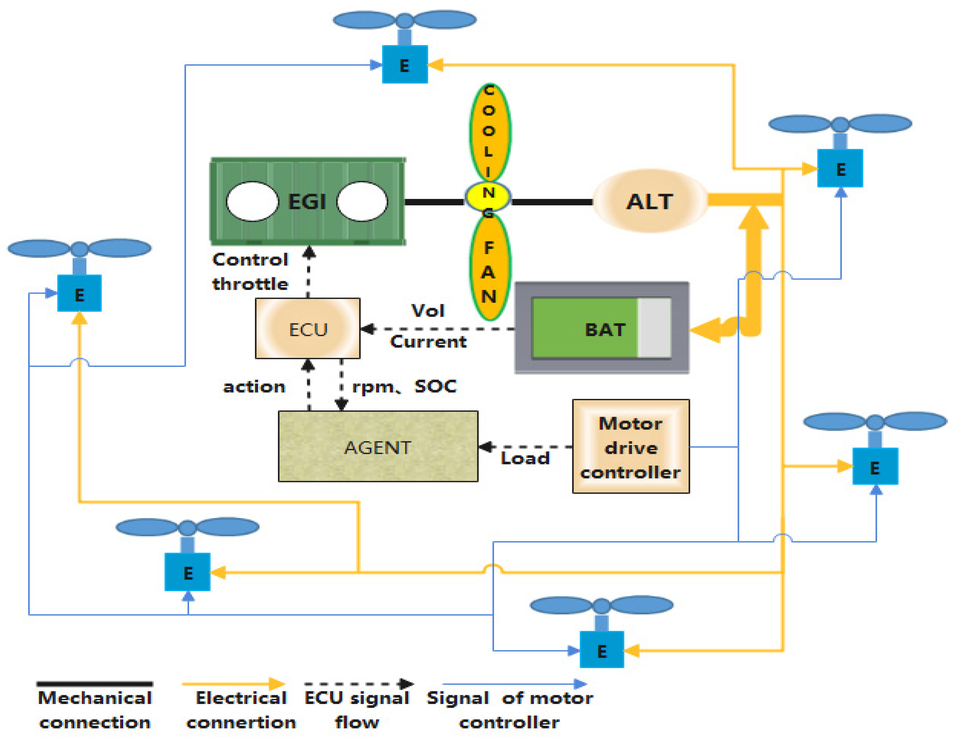
2.1. Hybrid System Modeling

Hybrid power systems usually consist of fuel and a battery. Considering the energy density and light weight, the range-extended propulsion system developed by our research group is composed of a two-stroke piston engine power generation system and a lithium battery in parallel. In this system, the internal combustion engine does not output power directly, but generates the power through a brushless motor and transmits the electric energy to the drive motor of each rotor of the UAV. At the same time, it can also store the excess electric energy in the lithium battery. In the control aspect, the processor processes the lithium battery status signal and Hall sensor electrical signal, and then transmits them to the agent as the speed of internal combustion engine and the state of charge (SOC) of energy storage device. The agent gives the control decision feedback to the Electronic Control Unit (ECU) combined with the load signal transmitted by the drive motor controller, and the ECU controls the throttle opening of internal combustion engine. The power system model is shown in Figure 1, and the main parameters of system components are shown in Table 1.

2.2. Internal Combustion Engine Modeling

Because only the input and output characteristics of the engine need to be obtained in the research process, the decision-making oriented experimental data modeling method is adopted for the engine [25]. The external characteristic data of the engine is obtained through testing, and the non-linear relationship of the working parameters is expressed by methods involving look-up tables and interpolation.
{ T E = f T ( n E , θ ) b E = f m f ( n E , T E )
where T E is the engine torque; n E is the working speed of the engine; θ is the engine throttle opening; b E is the fuel consumption rate of the engine.
The fuel consumption per unit step is obtained by integration:
fuel = 0 T P E · b E · Cd t
where P E is the engine power; C is a constant; b E is the fuel consumption rate of the engine.

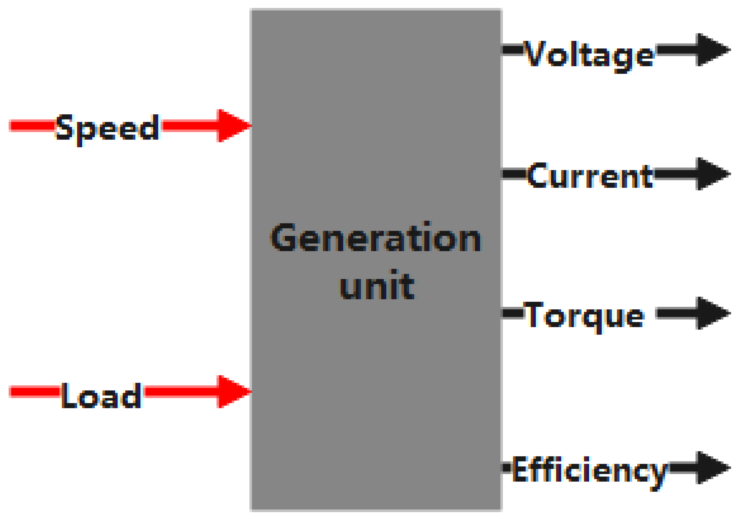
2.3. Generator Modeling

The motor used in the study is a permanent magnet synchronous motor. In order to facilitate the simulation and test, the generator and rectifier are modeled as a whole generation unit. As shown in Figure 2, in the modeling process, the load is converted into an equivalent resistance value, and, together with the speed of the motor, is used as the input of the generation unit. The output includes the reverse torque of the generator, the output voltage/current of the rectifier, and the generation efficiency. Under different loads and speeds, the output characteristics of the generating unit can be obtained by looking up the experimental data. The test bench is shown in Figure 3, and the test method involves the use of a high-power motor to drive the generator to rotate. The current output end is connected with resistors with different resistance values to simulate different working conditions. The speed can be displayed in real time. The external rotor of the generator is connected with the driving motor by coupling, the generator stator is connected with the test bench, and the torque sensor is connected with it to measure the reverse torque of the generator. The output current of the generator flows to the load after passing through the three-phase rectifier circuit.
The efficiency of the generating unit is obtained by dividing the output power of the rectifier by the input power of the generator:
η = I A × U A T A × n E / 9549
where U A and I A are the output voltage and output current; T A is the torque of the alternator; n E is the working speed of the engine.

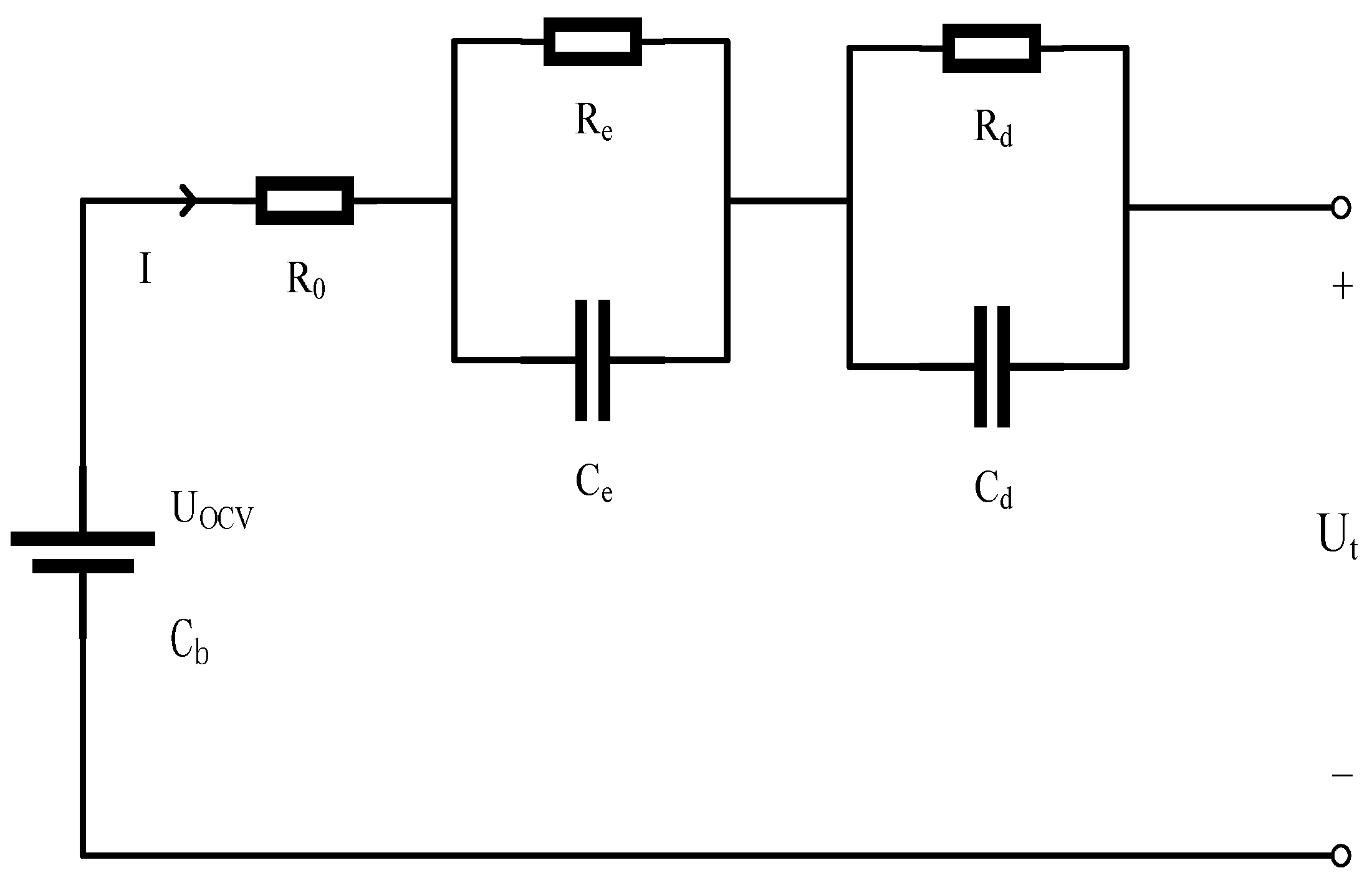
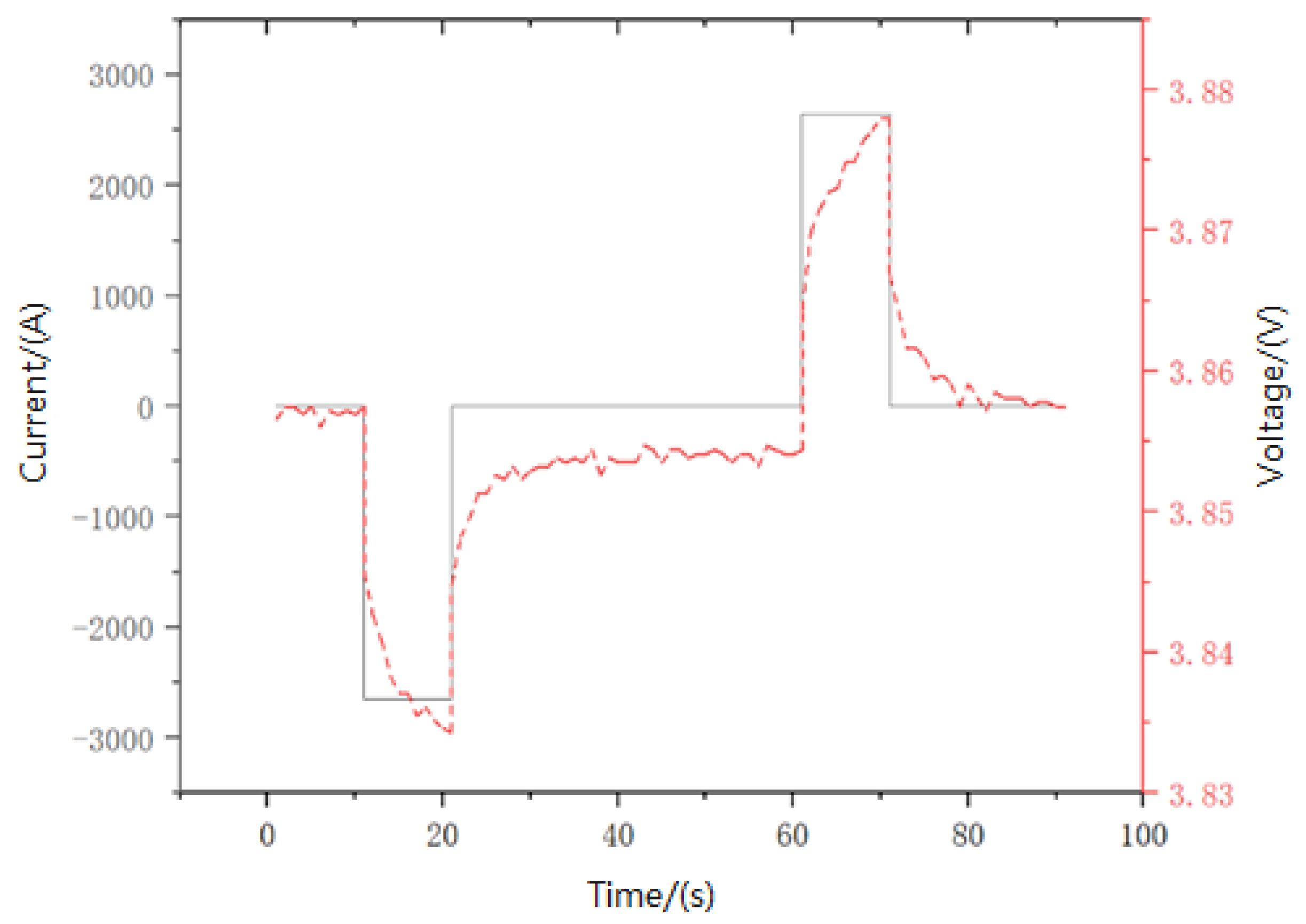
2.4. Energy Storage Device Modeling

In order to accurately describe the energy storage system, the second-order Thevenin model [26] is used to describe the battery. Owing to the addition of one RC circuit, the electrochemical polarization and concentration polarization of the battery can be accurately simulated. The circuit model is shown in Figure 4, where UOCV represents the open circuit voltage of the battery; Cb indicates the energy storage capacity of the battery; R0 represents the ohmic internal resistance of the battery; RE and CE represent the electrochemical polarization resistance and capacitance of the battery; Rd and Cd each represent the concentration polarization resistance and capacitance of the battery. Figure 5 shows the Hybrid Pulse Power Characteristic (HPPC) test data when the SOC is 0.6. When the current in the figure is negative, it is indicated that the battery is discharging, and when it is positive, it is indicated that the battery is charging. The voltage rises slowly after the battery discharge, which can be used as the zero input response of the battery model.
[ S ˙ O C U ˙ e U ˙ d U t ] = [ η C b I 1 R e C e U e + 1 C e I 1 R d C d U d + 1 C d I U O C V ( S O C ) I R 0 U e U d ]
where η is the efficiency of the battery in the charge and discharge state; U t is the output voltage of the lithium battery; I is the current; U e and U d are the voltage of electrochemical polarization and concentration polarization.
Through the polynomial fitting of the test data, the relationship between the SOC and OCV is obtained. The specific values of the parameters in the battery model under different states of charge are identified by the Hybrid Pulse Power Characteristic experiment.

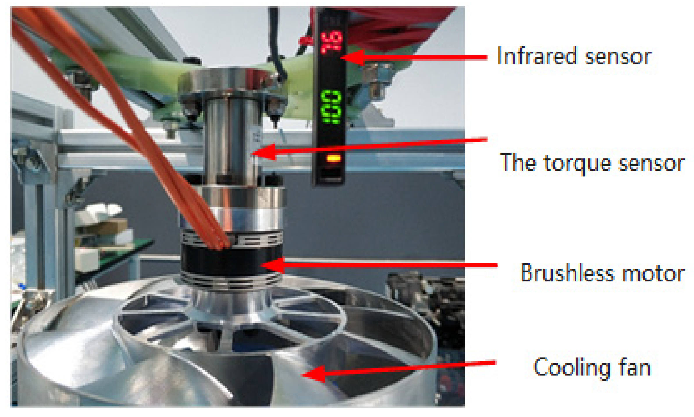
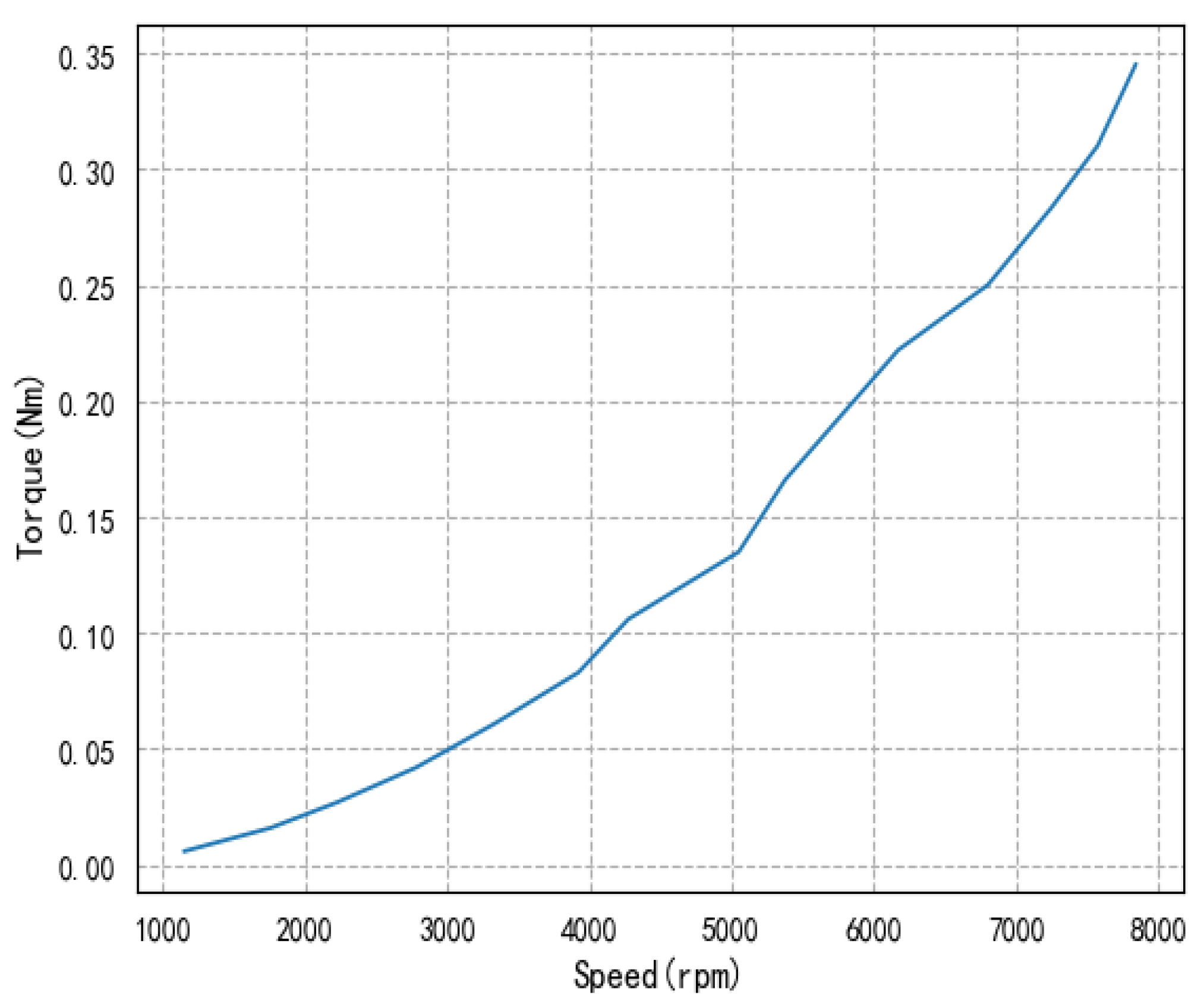
2.5. Cooling System Modeling

In the power system, the cooling fan is driven to rotate by connecting with the engine output shaft. At the same time, the cooling air duct is used to cool the cylinder block of the internal combustion engine. Because the research object of this paper is in low altitude flight, the influence of wind speed on the cooling fan can be ignored; thus, the relationship between the speed and power consumption is obtained through the ground experiment in Figure 6 by using the brushless motor to drive the cooling fan to rotate. The relationship curve is shown in Figure 7.

3. Energy Management Strategy

3.1. Introduction

In sequential decision problems, the Markov decision model (MDP) [27,28,29] is a mathematical model that simulates the randomness strategy and return of agents when the system state has Markov properties. The Markov property is a common property of all Markov models, which means that the current state is only related to the state and action of the previous discrete time point, and is independent of the state and action of other times. In the existing decision-making model, it can promptly discard useless historical information and avoid excessive processing of signal coupling, which helps it to take the lead in terms of the learning efficiency and effectiveness of random strategies. While simplifying the problem, it retains the main relationship, and can predict the future only based on the one-step dynamics of the environment. With its great simplicity and efficiency in the research process, some environments that do not fully have Markov properties have also been modeled by scholars using MDP, and have achieved good results.
p ( s i + 1 | s i , a i , , s 0 , a 0 ) = p ( s i + 1 | s i , a i )
The reinforcement learning algorithm is an intelligent algorithm to solve the cumulative revenue problem under discrete-time MDP. In this paper, we adopt the double Q learning algorithm, which is derived from the Q-Learning algorithm in the reinforcement learning algorithm family. The algorithm mainly includes three objects: the actor, the environment and the reward. Just like in Figure 8, the actor applies the action at at the current discrete time point to the environment and takes it as input together with the current state St in each interaction between the agent and the environment, and then the agent observes a new state S t + 1 of the environment at the next discrete time point and receives a reward r t + 1 as output. Under the action of the given strategy π ( a | s ) of the agent, the environment evolves from the initial state to the final state. In the process of continuous interaction between agents and the environment (Figure 8), the MDP trajectory, as shown below, is formed, which is a collection of all actions, states and rewards.
A τ = { s 0 , a 0 , r 1 , s 1 , a 1 , r 2 , s 2 , a 2 , , s T 1 , a T 1 , r T , s T }
where T is terminal discrete time point; s 0 is the initial state; s T is the terminal status. Due to the randomness of the strategy and state transition, the Markov trajectory also has randomness, and the probability is as follows:
p ( A τ ) = p ( s 0 ) i = 0 T 1 π ( a i | s i ) p ( s i + 1 | s i , a i )
where p ( s 0 ) obey the initial state distribution; π ( a i | s i ) refers to the probability that the strategy π selects action a i at state s i . The purpose of continuous interaction between actor and environment is to learn the best strategy and maximize the long-term benefits.
Under strategy π , the degrees of preference for taking different actions in a specific state S are quantified into specific values and expressed by function Q(s,a), which is the expected return after the state action pair appears in the MDP trajectory. Furthermore, the discount factor γ is used to ensure that the cumulative revenue under continuous tasks is bounded. With more and more returns observed, the average value will converge to the expected value:
Return ( S t , a t ) = i = t + 1 T γ i + 1 t r
Q ( S t , a t )     average   ( Returns ( S t , a t ) )
The function values of discrete state action pairs are stored in the agent in the form of a table (Q list).
When the result distribution of different actions is unknown in the model-free [30] situation, which means the probability distribution of the next state S’ can not be obtained, the state action value function Q(s,a) help in choosing the next action only by knowing the current state information. This caters well to the characteristics of instability and uncertainty of power demand in the practical application process, which is also the main reason that the control effect of hybrid EMS has been greatly limited for a long time. In addition, this paper aims to solve the flight time problem of UAV under variable operating conditions, so the total fuel consumption under the complete operating cycle is taken as the minimization objective, which is consistent with the cumulative revenue problem.

3.2. MDP Action and State Space

In the Markov Decision Process, the state space refers to a group of parameters with limited dimensions. It is used for the description of environmental information and action selection. The more parameters in the state space, the more accurate the description of the environment and the stronger the reliability. However, with the increase in dimensions, the computational burden will be greatly increased, and the convergence speed will be greatly reduced. From the perspective of effects in terms of practical application, the gain is not worth the loss. Therefore, it is very important to select the appropriate state variables in the limited state space dimension. According to the characteristics of the research objective and its application scenario, the speed, lithium battery state of charge, flight time and power demand of the small internal combustion engine are selected as a state space group, while the speed, lithium battery state of charge, remaining fuel and power of small internal combustion engine are selected as another state space group for comparison and analysis.
S 1 = { s = [ p , t , v , o ] T | p P , t T , v V , o O }
S 2 = { s = [ p , f , v , o ] T | p P , f F , v V , o O }
where P and V each represent the array of discrete power demand and internal combustion engine speed values; T and F each represent the array of discrete flight time and remaining fuel values and the elements in each array form an arithmetic sequence; O is the discrete value array of the lithium battery charge level.
In reinforcement learning theory, the role of strategy π is to determine the agent’s choice of action at different times. The ultimate goal of agent learning is to find the best strategy to maximize its long-term benefits.
a π ( a i | s t ) = 1
where π ( a i | s t ) represents the probability of selecting action a i in state s t under strategy π .
The improvement of the strategy is usually based on its corresponding value function Q π ( S t , a ) . When the function Q ( S t , a ) converges to the current strategy π , we can use it as a reference to optimize the strategy as below:
π n e w ( argmax a Q π ( S t , a ) | S t ) = 1
π n e w ( argmax a Q π ( S t , a ) | S t ) = 1 σ
where the former situation in Formula (13) is for deterministic strategies; the latter case in Formula (14) is for the randomness strategy and σ is usually set to a small probability to ensure the exploration of other actions.
The research objective of this paper includes two kinds of energy sources. The role of the power system control strategy is to coordinate the energy between the two on the premise of ensuring the power output. Because the generator and the output shaft of the internal combustion engine are mechanically connected in the system, the required power P dem needs to be distributed between the power generation system and the lithium battery ( P b a t , P A l ) . In this paper, the throttle opening of the internal combustion engine is regarded as the only action variable, and the output power of the alternator is changed by its control. Furthermore, the output power of the energy storage device P b a t is determined by the load signal transmitted to the ECU from the controller of the driving motor under the rotor and the P A l , which indirectly takes advantage of the fast response speed of the battery to ensure the dynamic performance of the system. The discrete action set is as follows, where a i represents the throttle opening in the actionable region.
A = { a 1 , a 2 , a 3 a k }

3.3. Reward Function

The setting of reward function can guide the optimal solution, and also has a certain impact on the algorithm quality and convergence speed. The purpose of this paper is to extend the flight time by reducing the fuel consumption of the hybrid system, so the negative value of fuel consumption per step r k + 1 is taken as the benefit. At the same time, in order to ensure the service life of lithium battery and avoid overcharge and discharge, a revenue punishment mechanism is set here: when the charge of energy storage device deviates from the healthy range (less than 20% or more than 80%), a larger penalty is given to the corresponding state action group as revenue.
r k + 1 = T K T K + 1 m f d t
where m f is instantaneous fuel consumption rate; T K is the time corresponding to state S K ; T K + 1 is the time corresponding to state S K + 1 .

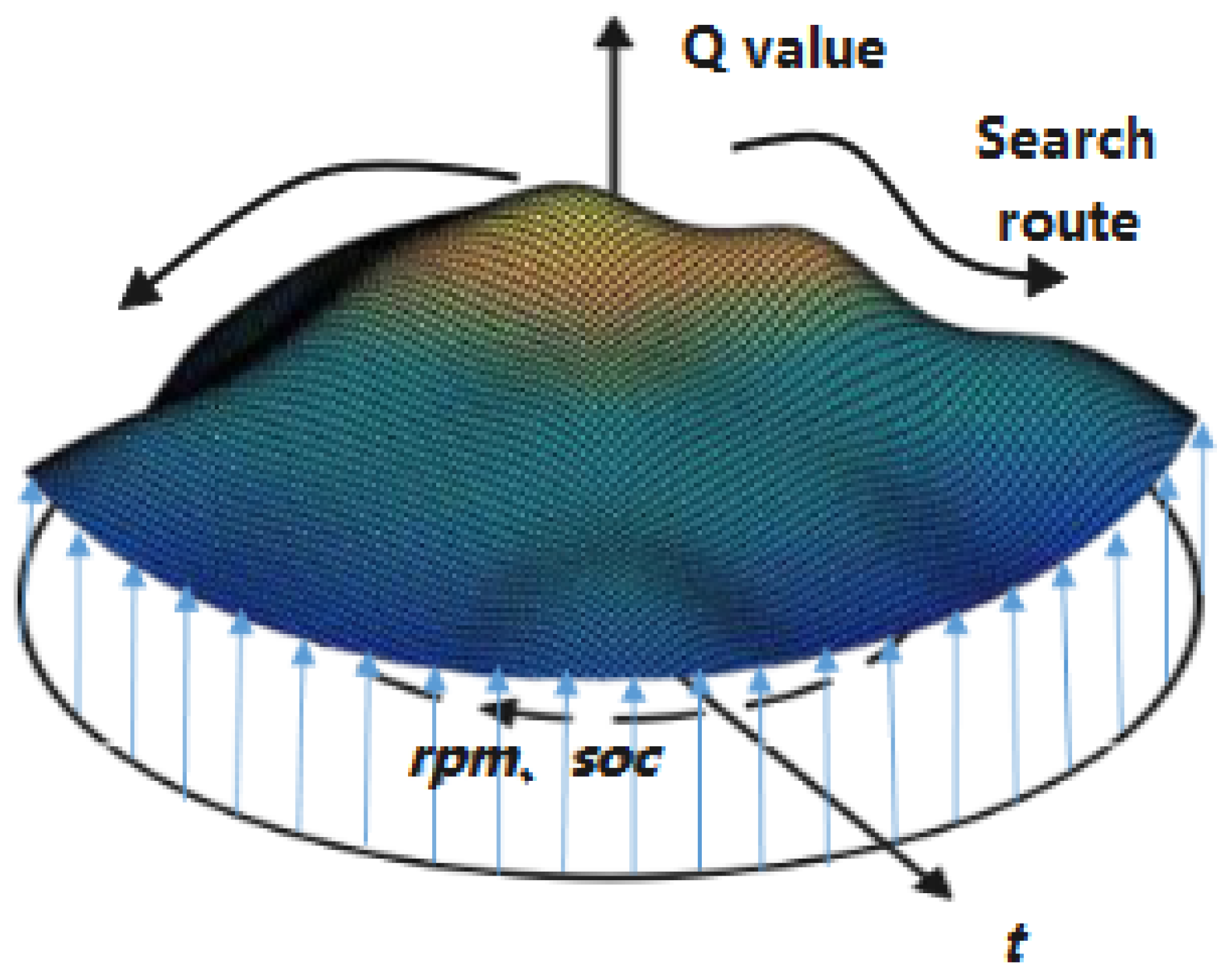
3.4. Theoretical Basis

Due to the uncertainty of working conditions and the wide range of states, the Markov decision model can not be obtained, which means that the state transition probability Function T P F is unknown.
T P F : S × A × S [ 0 , 1 ]
where the first S and A in the formula represent the current state and the action that has been performed, and the second S and [0, 1] represent all the different states that the environment can present at the next moment and their corresponding probabilities between 0 and 1. Furthermore, this inevitably leads to the failure to calculate the state value function under the given strategy; Q Learning [31,32,33] wisely uses experience to solve the problem of model prediction. To put it another way, its learning of the value function occurs through the expectation of samples rather than direct calculation. Each interaction sample between the agent and the environment produces an update to the table, as shown in the following formula:
Q ( S t , a t ) Q ( S t , a t ) + α [ r + γ argmax a Q ( S t + 1 , a ) Q ( S t , a t ) ]
where the discount factor γ is used to ensure that the cumulative revenue under continuous tasks is bounded; r is the reward; the update speed is determined by the learning efficiency a ; S t is the state of the environment at discrete time point t while a t is the action taken at the state S t ; a is the action used to generate the update target r + γ argmax a Q ( S t + 1 , a ) . With the continuous interaction between the agents and the environment under the control of strategy π , the list continues to update and gradually converges to the Q function of strategy π .
Because the Q ( S , a ) is only an estimate of the value of the pair of state actions under the policy, not the real value, the implicit maximum estimation will be propagated backward along the Markov trajectory by the item r + γ argmax a Q ( S t + 1 , a ) in Formula (8), which will produce a great obstacle to the convergence speed. In Table 2, double Q learning algorithm divides the Q list into two sets (Q1 and Q2) and uses them to learn the real Q functions (Table 2, line: 01). We obtain the maximum action A * from one Q list and use it to generate the update target from another Q list, and the two lists exchange roles with the same probability (Table 2, line: 10–13). The double learning method needs twice the chip memory, but it can achieve the purpose of using unbiased estimation instead of biased estimation on the premise of avoiding the enlargement of the computational burden, which greatly increases the learning speed.
In Table 2, we can see that in every discrete time point from the beginning of the initial state to the final state (Table 2, line: 03), the agent chooses the action guided by the maximum Q value with a large probability σ (Table 2, line: 05–06), while other state action spaces are explored with a small probability 1 σ (Table 2, line: 07–08). After interacting with the environment and obtaining the output (Table 2, line: 09), an update is generated to the Q function (Table 2, line: 10–13).
In the double Q learning algorithm, with each time step, the choice of strategy for action changes because of the update of the Q function (Table 2, line: 10–13) by the sample in the previous step ( S t 1 , a t 1 , r t , S t ) , rather than changing the strategy when the Q function converges to Q π ( S , a ) of the current strategy, as mentioned in Section 3.2. This is supported by the theory of generalized strategy iteration (GPI) [34,35], which is also the application basis of model-free Markov decision process [30]. As shown in Figure 9, the agent alternately evaluates the value function (Table 2, line: 10–13) and obeys the greedy-strategy guided by the Q function (Table 2, line: 05–06) step by step. Thus, the strategy can choose the most valuable action with high probability 1 σ in each state while continuing to update and explore the Q function value of other state action pairs with probability σ . The two processes influence each other and establish optimization goals for each other. According to the theory of GPI, they will move towards the optimal strategy and its Q function with the advance of the agent learning process.

3.5. Algorithm Improvement and Application

However, the convergence speed of the strategy and algorithm is important for its practical application. In the process of finding the optimal strategy, the agent needs to traverse the vast state action space, and the improvement of the strategy is also the process of increasing the value of the Q function. This paper adopts the idea of a fixed strategy search and refines the high return areas (state action pairs) of the Q list in the middle and later stages of the learning process, which can help to lock the decision-making route in the high return area earlier, so as to improve the sample efficiency and control effect of learned strategies π at the end of the learning process.
In the pseudo code of the improved algorithm (Table 3), we add the integer variable Episodes and database Rewards (Table 3, line: 01) in order to track the number of refinements happening in the Q list and the cumulative income of the trajectory chain before each refinement. After 40,000 Markov trajectories, the reward of the whole trajectory is compared with that before the last mesh refinement every 10,000 scenes (Table 3, line: 04, 18). If the income increases by 10%, the high return will be further refined (Table 3, line: 18–20), which means more state action pairs are added in the high return area of the Q list to obtain a discrete ( S , a ) group with smaller intervals, so that the agent can have more accurate state positioning and finer action selection. At the same time, the agent is free from the exploration and traversal of dense discrete state action pairs with low Q value.
In the algorithm application framework of Figure 10, the agent selects actions a t of throttle opening in a greedy manner according to two Q lists (Table 3, line: 08–11) in the current state St. After receiving the signal, the ECU transmits it to the steering gear to control the internal combustion engine. At the end of a time step, the identified SOC, internal combustion engine speed (RPM) and drive motor load (P) will be used as the next state quantity St+1 together with the flight progress information (Table 3, line: 12). Meanwhile, the engine fuel consumption model in the ECU, with engine speed and torque as input, calculates the total fuel consumption in this step time, and its negative value will be used as a reward rt+1 (Table 3, line: 12). Subsequently, the Q1 list and Q2 list in the agent will be updated randomly with equal probability (Table 3, line: 13–16), and the selection of the next action (Table 3, line: 17, 08–11) also begins. The above process circulates in each Markov trajectory until the end, and the agent starts to track the revenue and prepares to refine the Q1 and Q2 list every 10,000 trajectories (Table 3, line: 04–05, 18–20).

4. Results and Discussion

In the process of simulation, this paper uses the power demand curve obtained from the real historical flight data to train the control strategy algorithm, including 76 long- time-flights and 112 short-time flights. According to the frequency of the corresponding flight tasks in the actual flight of the UAV, the power demand curves are sorted randomly, and the agents are allowed to learn repeatedly. After reaching a certain degree of convergence, the learning effect is tested by the historical flight curve independent of the training samples. This part compares and analyzes the economy and convergence speed of the algorithm’s learning effect under different application modes, including the design of state variables, the comparison of the improved double Q learning method and original learning method, and the selection of charging and discharging frequency control functions. Finally, taking the global optimal result obtained by dynamic programming algorithm as the standard, the calculation cost and economy are evaluated and the practical application value is discussed.

4.1. Convergence Analysis

According to the previous discussion in this paper, the following figure is the comparison of the simulation test results of the improved learning models of double Q search learning, double Q learning and Q learning. The classification of the state action space and the setting of the initial function value of the three learning models are completely consistent. Figure 11 shows the comparison results of the total reward of a single trajectory after every 40,000 flight trajectories of training. At the beginning of learning, the state action value function and greedy factor ξ are set as smaller to ensure a larger exploration rate in the early stage. With the passage of time, the agent gradually enters the training stage, and the growth rate of the average income of the learning model gradually slows down. It is worth noting that in the improved double Q learning strategy, as the learning process goes on, every refinement of the state action space of the high return area can bring a promotion of revenue growth. Here, the new table function values of the high return area are equal to the Q function value of the state action pair with the smallest difference from its norm value.
Compared with Q-Learning, the double Q-Learning model is more effective owing to the ingenious avoidance of the obstruction of convergence speed caused by the maximization of deviation. Furthermore, the fluctuation of the average income data is greatly reduced, especially in the early stage. We can see from Table 4 that in the early training process, the variance of the whole screen return of Q learning is several times or even dozens of times of that of double Q learning. Although the stability advantage of convergence gradually decreases with the passage of time, the double Q learning model fluctuates in a relatively small range in terms of the average trajectory return. In addition, it can be seen from the last line of Table 4 and Figure 12 that the improved double-Q learning model benefits from the improvement in the accuracy of the state action space that happens in the middle and later stages of the process, which causes the strategy to lock into the vicinity of the optimal solution more quickly, and shows better performance in terms of stability as well as improvements in the speed of the strategy.

4.2. Economic Analysis

In this section, the two state spaces proposed in 3.2 are, respectively, applied to the training model proposed in this paper, and the power curves in the same flight database mentioned above are used to train them. In order to compare the adaptive performance of the two state variables in an unknown environment, after 120,000 flight trajectories of training, three short-time and three long-time flight load curves from the historical flight data, independent of the training samples shown in Figure 13, are used to test the learning effect.
In the two state spaces, we set the state variable components of flight process information as the flight time and the remaining fuel volume, respectively (in the simulation process, it is assumed that UAV always carries the same mass of fuel at every take-off). From the simulation results in Figure 14 and Figure 15 and Table 5, we can see that the description effect of flight time in short flights is better than that of remaining fuel. The reasons for this phenomenon are as follows: 1. In short-time flights, the correlation coefficient between the flight process and time is relatively large because the total times of cycle consumption are similar and the load curve is relatively stable. 2. In the training process of the learning model based on the remaining fuel, the state space of the agent is separated from the description of the real flight process, and due to the greedy selection in the same orbit strategy algorithm, it will produce a biased estimation of the real flight process with the Q function value learned from a large amount of flight data as the reference. As a result, the fuel consumption of different missions tends to approach the average fuel consumption of the simulation results of the working cycle in the training database, thus breaking away from the load characteristics of strange working conditions 3. The state space, which takes the actual flight time as the flight process information, also contains the current energy source states of the hybrid power system and the required power of the whole machine. In the energy management problem, it is a complete description that includes unknown environmental state information, and ignores the influence of previous sequential decisions on the moment; thus, the near optimal decision generated from Q list of the historical flight data will give full play to the advantages of Markov decision model. In addition, due to the fact that the fuel volume state is not always equal before each short-time flight mission, there are also some problems related to the practical application of the controller.
In view of the large variance of flight time in the actual long-time flight mission, in order to test the robustness of the learning effect, three load curves with long discrete flight times are selected to test the control strategy. In the Figure 16 and Figure 17, we can see the learning effects of two different state spaces under long-time flight trajectories, which shows good performance in terms of both operating point optimization and economy. The reason is that the time parameter will give more and more warning of the end of the flight mission as the flight process goes on. Because of the enhancement of this notice, the controller tends to complete the remaining flight in a more fuel-efficient manner, that is, more electric energy is obtained from the energy storage device and supplied to the terminal drive motor, which leads to the disorder of the regulation function of the working point in the later flight period under the changeable environment. It deviates from the purpose of exerting the endurance of the power system in long-time flights. However, in the case of variable flight trajectories, the learning model with remaining fuel as the source of information on progress obtains the action of any time point from the Q list according to the greedy strategy, and the action is the result of many ergodic measures of the state in the past training. This kind of ergodicity can, at any time, be under any working condition. Its optimal action is to lock the operating point of the internal combustion engine in the high efficiency region to the greatest extent in the future flight process. Thus, in the long-time flight problem, compared with the short-flight time, the state space with the remaining fuel as the flight process information can show better effect.

4.3. Charge–Discharge Frequency Analysis

In the process of learning, the SOC of the lithium battery in power system is tracked and recorded. With the increasing density of discrete points in the state action space, the intelligent agent has more flexible choice for the system working mode at each time, which increases the charging and discharging frequency of lithium battery and poses a threat to the health of the battery. Here, a Smode (SCHA, SDISCHA) variable is added to the state space as the working mode identification, in which the SCHA indicates that the lithium battery is in the state of charge and SDISCHA means that the lithium battery is in the discharge state. Smode is identified by comparing the output power of the current generation system with the power required for the drive motor at the end of each step. When Smode is different at the beginning and end of a step, a negative revenue value r mode is added to the updated target of the value function as the punishment, and the punishment value determines the strength of the limitation of the charge–discharge conversion frequency.
Q ( S , A ) Q ( S , A ) + α [ r + r mode + γ × max a Q ( S , A ) Q ( S , A ) ]
Of course, it is not excluded that the variable is transformed twice in one step, which can help to successfully escape punishment for learning models. Because of the low probability of this situation and considering the economy and calculation cost of EMS, we choose to ignore it. Even then we can see in Figure 18 that with the increase in penalties on S mode, the regulation capacity of the energy storage device and the conversion frequency of the working mode show a downward trend.

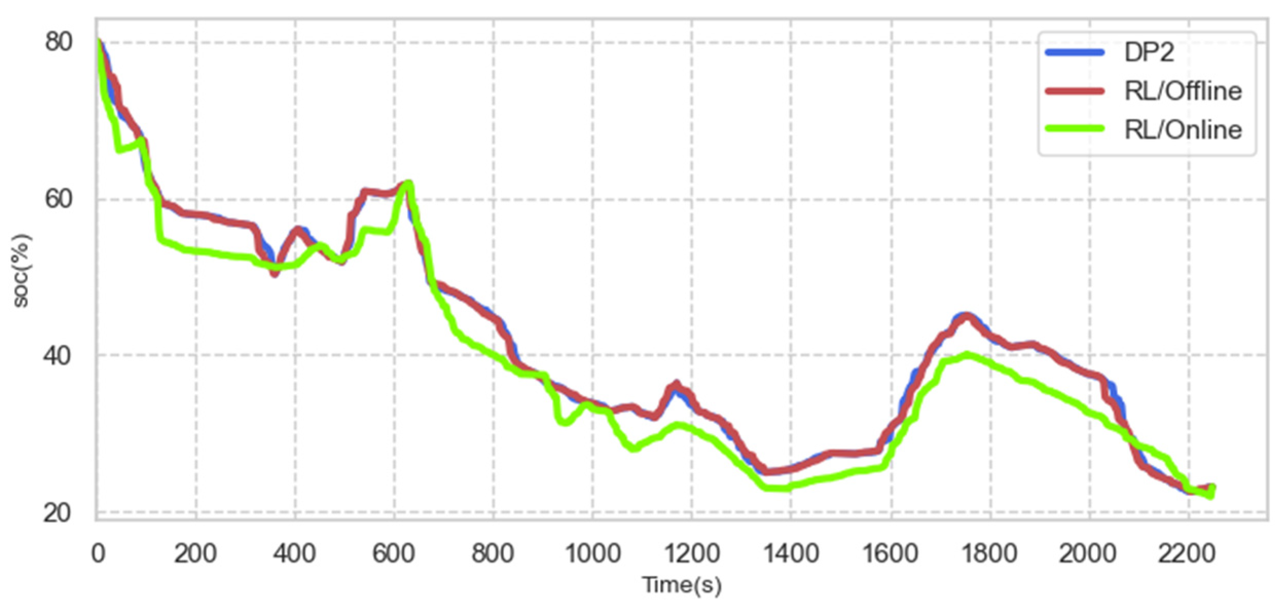
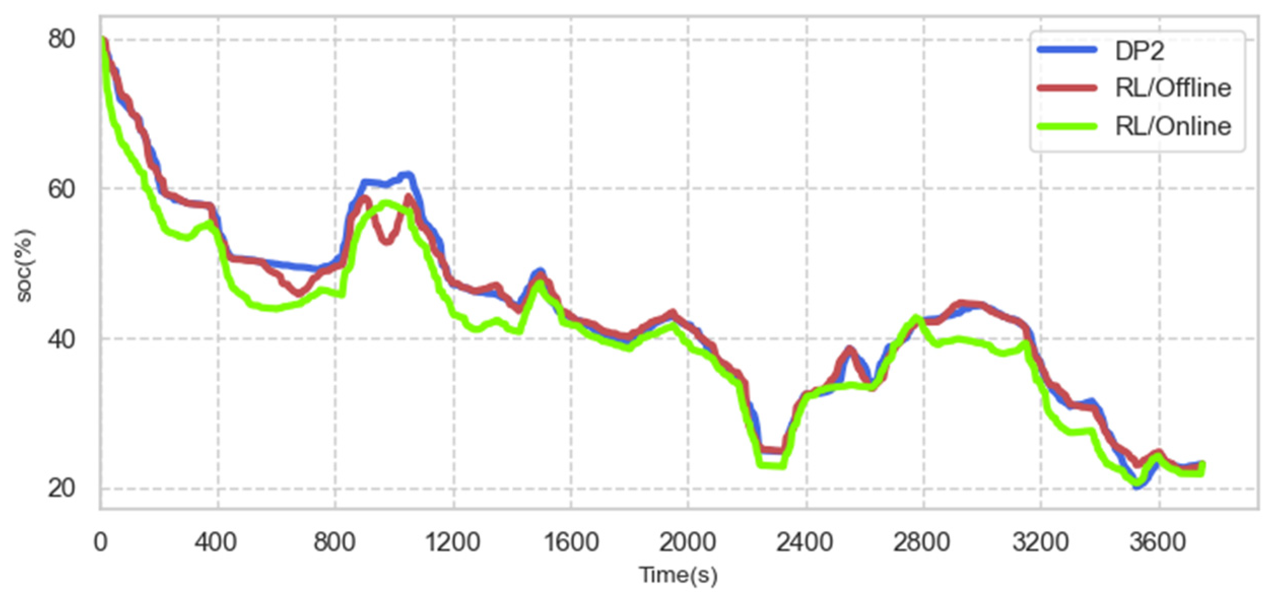
4.4. On-Line Control Analysis

In order to verify the effectiveness of the on-line control, we test the trained control strategy on-line and off-line in two different conditions using the UAV in Figure 19. In the actual flight process of the UAV, the calculation speed of the control strategy is greatly increased by establishing a communication relationship between the flight control system in Figure 20 and the ground high-performance server. In the actual flight, the average inference time of a decision is 3.03 ms, which is far less than that of one time step.
In Table 6, the control effect of learning results under unfamiliar conditions is compared with the two kinds of dynamic programming methods with different precision and rules-based methods: for the DP2 based on dynamic programming with the same state precision as the RL method used in this paper (the state precision of RL method refers to the state precision of high return area at the end of strategy search), in the final test results of two unfamiliar conditions, RL can achieve 94.86% and 97.67% economy, respectively, compared to that of DP2, and the calculation time is reduced by about half. Compared with the rule-based EMS, the RL method in this paper saves 22.90% and 17.90% of the fuel consumption, respectively, under two unfamiliar conditions. The above results show that the designed EMS scheme can work effectively and stably under different working conditions. In this paper, we try to transfer the optimal decision sequences of two very similar power curves to each other using the DP1 method, but the economy can only reach 82.31% and 77.57%, respectively, compared with the RL method. The reason is that RL method stores a vast amount of state action value information with efficient training, followed by the infinite approximation of the optimal Q function. With the increase in the number of training scenes, the universality of the load curve also increases greatly, which guarantees the approximation performance for the optimal decision route as shown in the Figure 21 and Figure 22. The essence of the dynamic programming method is to solve the global optimal problem under a specific cycle. Once the load curve changes to a certain extent, the grafting effect will be greatly reduced.

4.5. Conclusions

In this paper, the energy management strategy of an augmented UAV based on Q-Learning is studied and the following results can be obtained: (1) The reasonable selection of state space parameters for different types of flight missions can significantly improve the control effect. (2) After the improvement of the search type of the algorithm, the agent can quickly lock the learned decision path near the optimal solution. With the continuous refinement of the state action space, the energy management strategy can reduce the calculation cost and increase the economy. (3) In the actual flight test of the improved Q-Learning algorithm, each decision step is controlled at about only 3 ms by establishing the communication relationship with the high-performance server on the ground. Compared with the computer simulation, the control effect can reach more than 95% of the optimal value, which has considerable practical application value. Furthermore, from a large number of simulation results, we can see that the improved Q-Learning algorithm has great robustness and excellent performance in hybrid energy management compared with other algorithms. To a certain extent, it breaks the shortcomings of the existing control strategy in this field. In future research, we will introduce neural networks, and the improvement of empirical efficiency and error estimation will be taken as breakthrough points.

Author Contributions

Conceptualization, Y.Z. and Z.Y.; methodology, H.S. and Y.Z.; software, Z.Y.; validation, J.M. and L.W.; formal analysis, J.M. and Z.Y.; investigation, Y.Z.; resources, H.S.; data curation, L.W.; writing—original draft preparation, Y.Z.; writing—review and editing, H.S.; visualization, Z.Y.; supervision, J.M.; project administration, J.M. All authors have read and agreed to the published version of the manuscript.

Funding

This research received no external funding.

Conflicts of Interest

The authors declare no conflict of interest.

References

  1. Lei, T.; Min, Z.; Fu, H.; Zhang, X.; Li, W.; Zhang, X. Research on dynamic balance management strategy of hybrid power supply for fuel cell UAV. J. Aeronaut. 2020, 41, 324048. [Google Scholar]
  2. Sun, H.; Fu, Z.; Tao, F.; Zhu, L.; Si, P. Data-driven reinforcement-learning-based hierarchical energy management strategy for fuel cell/battery/ultracapacitor hybrid electric vehicles. J. Power Sources 2020, 455, 227964. [Google Scholar] [CrossRef]
  3. Xu, B.; Hu, X.; Tang, X.; Lin, X.; Rathod, D.; Filipi, Z. Ensemble Reinforcement Learning-Based Supervisory Control of Hybrid Electric Vehicle for Fuel Economy Improvement. IEEE Trans. Transp. Electrif. 2020, 6, 717–727. [Google Scholar] [CrossRef]
  4. Hajji, B.; Mellit, A.; Marco, T.; Rabhi, A.; Launay, J.; Naimi, S.E. Energy Management Strategy for parallel Hybrid Electric Vehicle Using Fuzzy Logic. Control Eng. Pract. 2003, 11, 171–177. [Google Scholar]
  5. Yang, C.; You, S.; Wang, W.; Li, L.; Xiang, C. A Stochastic Predictive Energy Management Strategy for Plug-in Hybrid Electric Vehicles Based on Fast Rolling Optimization. IEEE Trans. Ind. Electron. 2019, 67, 9659–9670. [Google Scholar] [CrossRef]
  6. Li, J.; Sun, Y.; Pang, Y.; Wu, C.; Yang, X. Energy management strategy optimization of hybrid electric vehicle based on parallel deep reinforcement learning. J. Chongqing Univ. Technol. (Nat. Sci.) 2020, 34, 62–72. [Google Scholar]
  7. Li, Y.; He, H.; Khajepour, A.; Wang, H.; Peng, J. Energy management for a power-split hybrid electricbus via deep reinforcement learning with terraininformation. Appl. Energy 2019, 255, 113762. [Google Scholar] [CrossRef]
  8. Hou, S.; Gao, J.; Zhang, Y.; Chen, M.; Shi, J.; Chen, H. A comparison study of battery size optimization and an energy management strategy for FCHEVs based on dynamic programming and convex programming. Int. J. Hydrogen Energy 2020, 45, 21858–21872. [Google Scholar] [CrossRef]
  9. Song, Z.; Hofmann, H.; Li, J.; Han, X.; Ouyang, M. Optimization for a hybrid energystorage system in electric vehicles using dynamic programing approach. Appl. Energy 2015, 139, 151–162. [Google Scholar] [CrossRef]
  10. Zou, Y.; Teng, L.; Sun, F.; Peng, H. Comparative study of dynamic programming and pontryagin minimum principle on energy management for a parallel hybridelectric vehicle. Energies 2013, 6, 2305–2318. [Google Scholar]
  11. Francesco, P.; Petronilla, F. Design of an Equivalent Consumption Minimization Strategy-Based Control in Relation to the Passenger Number for a Fuel Cell Tram Propulsion. Energies 2020, 13, 4010. [Google Scholar]
  12. Wu, Y.; Tan, H.; Peng, J.; Zhang, H.; He, H. Deep reinforcement learning of energy management with continuous control strategy and traffic information for a series-parallel plug-in hybrid electric bus. Appl. Energy 2019, 247, 454–466. [Google Scholar] [CrossRef]
  13. Xu, R.; Niu, L.; Shi, H.; Li, X.; Dou, H.; Pei, Z. Energy management optimization strategy of extended range electric vehicle. J. Anhui Univ. Technol. (Nat. Sci. Ed.) 2020, 37, 258–266. [Google Scholar]
  14. Gen, W.; Lou, D.; Zhang, T. Multi objective energy management strategy of hybrid electric vehicle based on particle swarm optimization. J. Tongji Univ. (Nat. Sci. Ed.) 2020, 48, 1030–1039. [Google Scholar]
  15. Hou, S. Research on Energy Management Strategy and Power Cell Optimization of Fuel Cell Electric Vehicle. Master’s Thesis, Jilin University, Jilin, China, 2020. [Google Scholar]
  16. Liu, C.; Murphey, Y.L. Optimal Power Management Based on Q-Learning and Neuro-Dynamic Programming for Plug in Hybrid Electric Vehicles. IEEE Trans. Neural Netw. Learn. Syst. 2020, 31, 1942–1954. [Google Scholar] [CrossRef]
  17. Park, J.; Chen, Z.; Kiliaris, L.; Kuang, M.L.; Masrur, M.A.; Phillips, A.M.; Murphey, Y.L. Intelligent vehicle power control based on machine learning of optimal control parameters and prediction of road type and traffic congestion. IEEE Trans. Veh. Technol. 2009, 58, 4741–4756. [Google Scholar] [CrossRef]
  18. Xu, B.; Rathod, D.; Zhang, D. Parametric study on reinforcement learning optimized energy management strategy for a hybrid electric vehicle. Appl. Energy 2020, 259, 114200. [Google Scholar] [CrossRef]
  19. Han, X.; He, H.; Wu, J.; Peng, J.; Li, Y. Energy management based on reinforcement learning with double deep Q-Learning for a hybrid electric tracked vehicle. Appl. Energy 2019, 254, 113708. [Google Scholar] [CrossRef]
  20. Qi, X.; Wu, G.; Boriboonsomsin, K.; Barth, M.J.; Gonder, J. Data-Driven Reinforcement Learning-Based Real-Time Energy Management System for Plug-In Hybrid Electric Vehicles. Transp. Res. Rec. 2016, 2572, 1–8. [Google Scholar] [CrossRef] [Green Version]
  21. Bai, M.; Yang, W.; Song, D.; Kosuda, M.; Szabo, S.; Lipovsky, P.; Kasaei, A. Research on Energy Management of Hybrid Unmanned Aerial Vehicles to Improve Energy-Saving and Emission Reduction Performance. Int. J. Environ. Res. Public Health 2020, 17, 2917. [Google Scholar] [CrossRef] [Green Version]
  22. Boukoberine, M.N.; Zhou, Z.B.; Benbouzid, M. A critical review on unmanned aerial vehicles power supply and energy management: Solutions, strategies, and prospects. Appl. Energy 2019, 255, 113823. [Google Scholar] [CrossRef]
  23. Arum, S.C.; Grace, D.; Mitchell, P.D.; Zakaria, M.D.; Morozs, N. Energy Management of Solar-Powered Aircraft-Based High Altitude Platform for Wireless Communications. Electronics 2020, 9, 179. [Google Scholar] [CrossRef] [Green Version]
  24. Lei, T.; Yang, Z.; Lin, Z.C.; Zhang, X.B. State of art on energy management strategy for hybrid-powered unmanned aerial vehicle. Chin. J. Aeronaut. 2019, 32, 1488–1503. [Google Scholar] [CrossRef]
  25. Cook, J.A.; Powell, B.K. Modeling of an internal combustion engine for control analysis. IEEE Control Syst. Mag. 1998, 8, 20–26. [Google Scholar] [CrossRef]
  26. Ding, X.; Zhang, D.; Cheng, J.; Wang, B.; Luk, P.C.K. An improved Thevenin model of lithium-ion battery with high accuracy for electric vehicles. Appl. Energy 2019, 254, 113615. [Google Scholar] [CrossRef]
  27. Bennett, C.C.; Hauser, K. Artificial intelligence framework for simulating clinical decision-making: A Markov decision process approach. Artif. Intell. Med. 2013, 57, 9–19. [Google Scholar] [CrossRef] [Green Version]
  28. White, C.C., III. A survey of solution techniques for the partially observed Markov decision process. Ann. Oper. Res. 1991, 32, 215–230. [Google Scholar] [CrossRef] [Green Version]
  29. Cipriano, L.E.; Goldhaber-Fiebert, J.D.; Liu, S.; Weber, T.A. Optimal Information Collection Policies in a Markov Decision Process Framework. Med. Decis. Mak. 2018, 38, 797–809. [Google Scholar] [CrossRef]
  30. Wei, C.Y.; Jahromi, M.J.; Luo, H.; Sharma, H.; Jain, R. Model-free Reinforcement Learning in Infinite-horizon Average-reward Markov Decision Processes. In Proceedings of the 37th International Conference on Machine Learning, Shanghai, China, 13–18 July 2020; Volume 119, pp. 10170–10180. [Google Scholar]
  31. Wang, Y.H.; Li, T.H.S.; Lin, C.J. Backward Q-Learning: The combination of Sarsa algorithm and Q-Learning. Eng. Appl. Artif. Intell. 2013, 26, 2184–2193. [Google Scholar] [CrossRef]
  32. He, Z.; Li, L.; Zheng, S.; Li, Y.; Situ, H. Variational quantum compiling with double Q-Learning. New J. Phys. 2021, 23, 033002–033016. [Google Scholar] [CrossRef]
  33. Liu, T.; Wang, B.; Yang, C. Online Markov Chain-based energy management for a hybrid tracked vehicle with speedy Q-Learning. Energy 2018, 160, 544–555. [Google Scholar] [CrossRef]
  34. Ji, T.; Zhang, H. Nonparametric Approximate Generalized strategy iterative reinforcement learning algorithm based on state clustering. Control Decis. Mak. 2017, 32, 12. [Google Scholar]
  35. Van Der Wal, J. Discounted Markov games: Generalized policy iteration method. J. Optim. Theory Appl. 1978, 25, 125–138. [Google Scholar] [CrossRef]
Figure 1. Propulsion system architecture of the UAV.
Electronics 10 01929 g001
Figure 2. Schematic diagram of input and output of power generation unit model.
Electronics 10 01929 g002
Figure 3. Generator testing bench.
Electronics 10 01929 g003
Figure 4. Battery pack model.
Electronics 10 01929 g004
Figure 5. HPPC test data diagram.
Electronics 10 01929 g005
Figure 6. Connection structure of test bench.
Electronics 10 01929 g006
Figure 7. Torque–speed curve of cooling fan.
Electronics 10 01929 g007
Figure 8. Agent and environment.
Electronics 10 01929 g008
Figure 9. Schematic diagram of algorithm iteration.
Electronics 10 01929 g009
Figure 10. Application framework of improved double Q algorithm.
Electronics 10 01929 g010
Figure 11. Learning effect of different algorithms.
Electronics 10 01929 g011
Figure 12. Value oriented search route.
Electronics 10 01929 g012
Figure 13. Test trajectories of learning effect: (a) short time trajectories; (b) long time trajectories.
Electronics 10 01929 g013
Figure 14. Comparison of operating points affected by different state spaces: (a) short time trajectories; (b) long time trajectories.
Electronics 10 01929 g014
Figure 15. State space distribution of short flight mission: (a) S2; (b) S1; (c) optimal.
Electronics 10 01929 g015
Figure 16. State space distribution of long flight mission: (a) S2; (b) S1; (c) optimal.
Electronics 10 01929 g016
Figure 17. Distribution statistics of operating points.
Electronics 10 01929 g017
Figure 18. Battery power curve.
Electronics 10 01929 g018
Figure 19. Real object drawing of multi rotor aircraft.
Electronics 10 01929 g019
Figure 20. Joint debugging of flight control system and ECU. (1—ECU; 2—ECU harness; 3—RS-232 to TTL photoelectric isolation converter; 4—flight control board; 5—digital transmission platform; 6—ground station).
Electronics 10 01929 g020
Figure 21. SOC tracking record of short flight mission.
Electronics 10 01929 g021
Figure 22. SOC tracking record of long flight mission.
Electronics 10 01929 g022
Table 1. Main design parameters of the system.
DeviceItemParameter
EngineCylinders2
Rated torque4.6 Nm
Power rating2.8 Kw
Rated speed2000–7200 rpm
AlternatorPower rating2.7 Kw
Phase resistance0.3 Ω
D-axis inductance0.09 mH
Q-axis inductance0.09 mH
BatteryTypeLi-Po Graphene
Capacity5.2 Ah
Voltage (single cell)4.2 V
Table 2. Pseudo code of the original double Q learning algorithm.
Inputs: 5-D Q ( S , a ) table; Discount factor γ ; Learning rate α ; Exploration probability σ
Outputs: near global optimal strategy
01: Initialize Q1 list and Q2 list arbitrarily;
02: for each MDP trajectory:
03:  for each discrete time step t = 0:T~1:
04:    observe the state S t ( o ,   p ,   t ,   v ) :
05:    if temp0 (a random number between 0 and 1) > σ :
06:      a t = argmax a ( Q 1 ( S t , a ) + Q 2 ( S t , a ) ) ;
07:    else:
08:      a t = randomly choose an action;
09:    Take action a t and observe the next state S t and r t + 1 ;
10:    If temp1 (a random number between 0 and 1) <= 0.5:
11:      Q 1 ( S t , a t ) = Q 1 ( S t , a t ) + α ( r t + 1 + γ Q 2 ( S t + 1 , argmax a Q 1 ( S t + 1 , a ) ) Q 1 ( S t , a t ) ) ;
12:    else:
13:      Q 2 ( S t , a t ) = Q 2 ( S t , a t ) + α ( r t + 1 + γ Q 1 ( S t + 1 , argmax a Q 2 ( S t + 1 , a ) ) Q 2 ( S t , a t ) ) ;
14:     S t = S t + 1 ;
Table 3. Pseudo code of the improved double Q algorithm.
Inputs: 5-D Q ( S , a ) table; Discount factor γ ; Learning rate α ; Exploration probability σ
Outputs: near global optimal strategy
01: Initialize Q 1 ( S , a ) and Q 2 ( S , a ) arbitrarily; Chain = Episodes = 0; Rewards = [−1000];
02: for each MDP trajectory:
03:  reward = 0;
04:  If Chain/40,000 = = 10,000:
05:    ε = 1 ;
06:  for each time step t = 1~T:
07:   observe the state S t ( o ,   p ,   t ,   v ) :
08:   if temp (= random(0,1)) > σ :
09:     a t = argmax a ( Q 1 ( S t , a ) + Q 2 ( S t , a ) ) ;
10:   else:
11:    at = randomly choose an action;
12:   Take action a t and observe the next state S t + 1 and r ; reward = reward + r ;
13:   If temp (= random(0,1)) <= 0.5:
14:     Q 1 ( S t , a t ) = Q 1 ( S t , a t ) + α ( r t + 1 + γ Q 2 ( S t + 1 , argmax a Q 1 ( S t + 1 , a ) ) Q 1 ( S t , a t ) ) ;
15:   else:
16:     Q 2 ( S t , a t ) = Q 2 ( S t , a t ) + α ( r t + 1 + γ Q 1 ( S t + 1 , argmax a Q 2 ( S t + 1 , a ) ) Q 2 ( S t , a t ) ) ;
17:    S t = S t + 1 ;
18:  If ε = 1 and reward/Reward [Episodes] < 0.9:
19:    Refine high Q table, ε = 0;
20:    Rewards.append (reward), Episodes = Episodes + 1;
21:  Chain = Chain + 1
Table 4. Convergence comparison of different algorithms.
Training Progress
(×400 Trajectories)
100–110200–210300–310400–410
Fuel consumptionaverage/varianceaverage/varianceaverage/varianceaverage/variance
Q Learning418.4 g/4007.7340.6 g/813.1301.6 g/237.1296.4 g/16.1
Double Q Learning355.4 g/1104.3298.6 g/51.9294.7 g/56.4290.2 g/8.7
Proposed double Q Learning320.4 g/137.1275.9 g/5.2263.2 g/1.8262.3 g/0.6
Note: g = grams.
Table 5. Total fuel consumption of single cycle.
Long Time Trajectory 1Long Time Trajectory 2Long Time Trajectory 3Short Time Trajectory 1Short Time Trajectory 2Short Time Trajectory 3
S1/g935.57966.481291.71388.88517.21451.07
S2/g879.63914.661235.05409.45552.67491.02
S1/S2106.36%105.67%104.59%94.59%93.58%91.86%
Note: g = grams.
Table 6. Comparison of application effects of different control strategies.
DP1DP2RLRULE-BSEDDP1-DP2/RL(%)RULE-BSED/RL(%)
OfflineOfflineOffline/ActualOffline
State and action accuracy0.010.0050.005
Fuel consumption under training condition A (short-time)467.31 g427.28 g440.78 g/-545.97 g106.02/96.94123.87
Fuel consumption under training condition B (long-time)982.34 g879.10 g937.80 g/-1083.03 g104.74/93.74115.49
Fuel consumption under strange condition A (short-time)455.98 g418.32 g447.32 g/429.82 g557.52 g101.84/93.51124.64
Fuel consumption under strange condition B (long-time)1142.57 g1036.38 g1140.51 g/1092.76 g1329.72 g100.18/90.87116.58
Average calculation cost18.6 h74.3 h37.0 h
Note: g = grams; h = hours.
Publisher’s Note: MDPI stays neutral with regard to jurisdictional claims in published maps and institutional affiliations.

