
Balancing Awareness and Congestion in Vehicular Networks Using Variable Transmission Power


Abstract
1. Introduction
2. Related Work
Existing Decentralized Congestion Control Approaches
3. The Balancing Awareness and Congestion Power Control Algorithm
3.1. Algorithm Design Methodology
3.2. Proposed Algorithm
| Algorithm 1: Balancing awareness and congestion with variable Tx power (BACVT) algorithm. |
 |
- All BSMS from the EV, if ;
- The BSMs transmitted with high Tx power (), if ;
- No BSMs from the EV, if .
3.2.1. Hybrid Approach
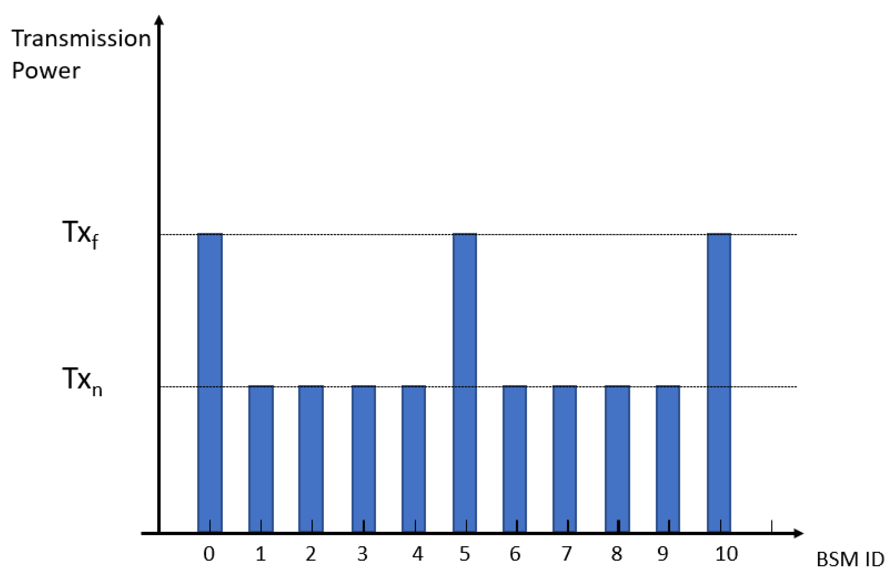
3.3. Illustrative Example
| Algorithm 2: A hybrid approach combined with random rate control (BACVT-H). |
 |
4. Simulation Results
4.1. Simulation Parameters
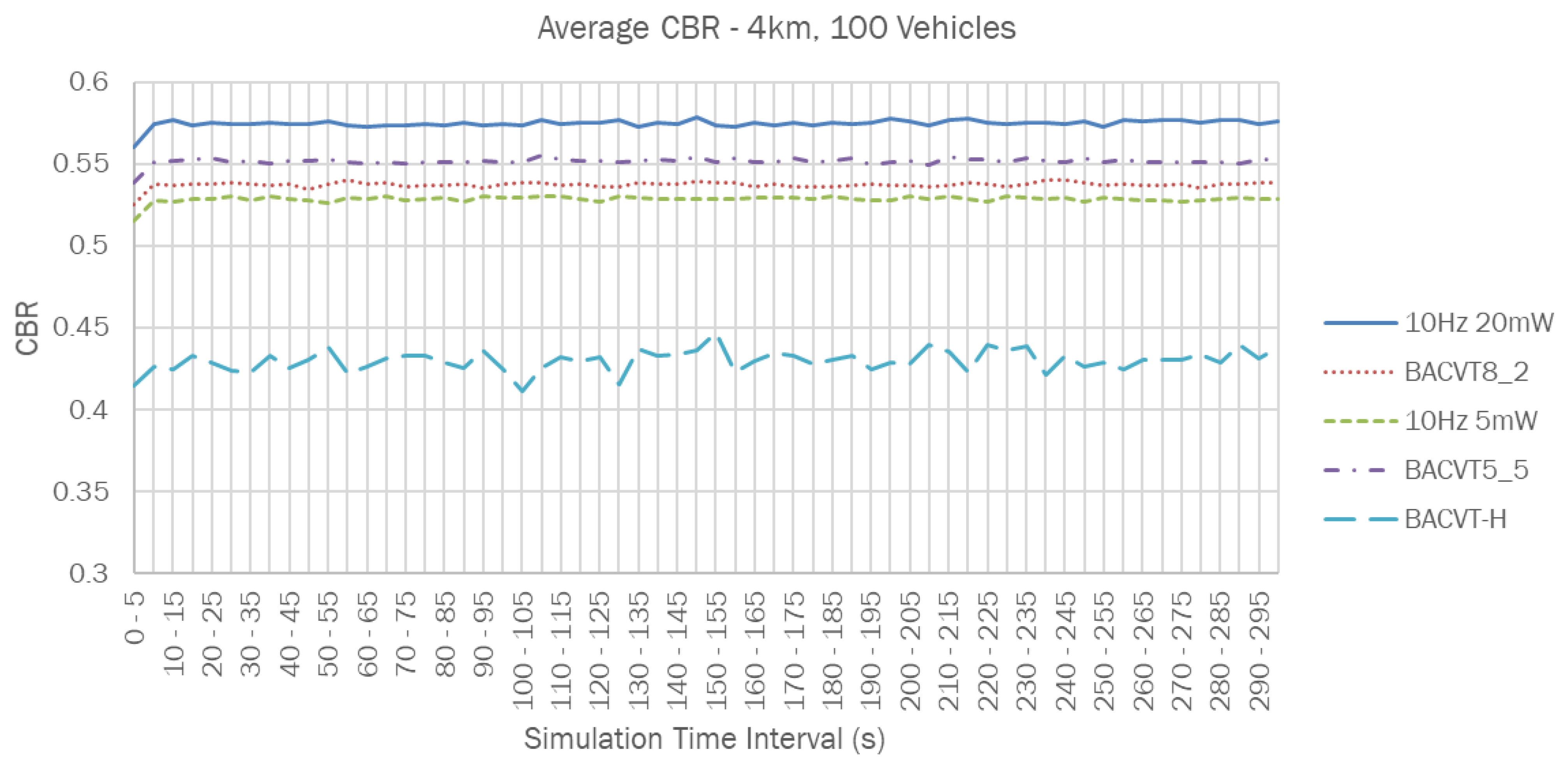
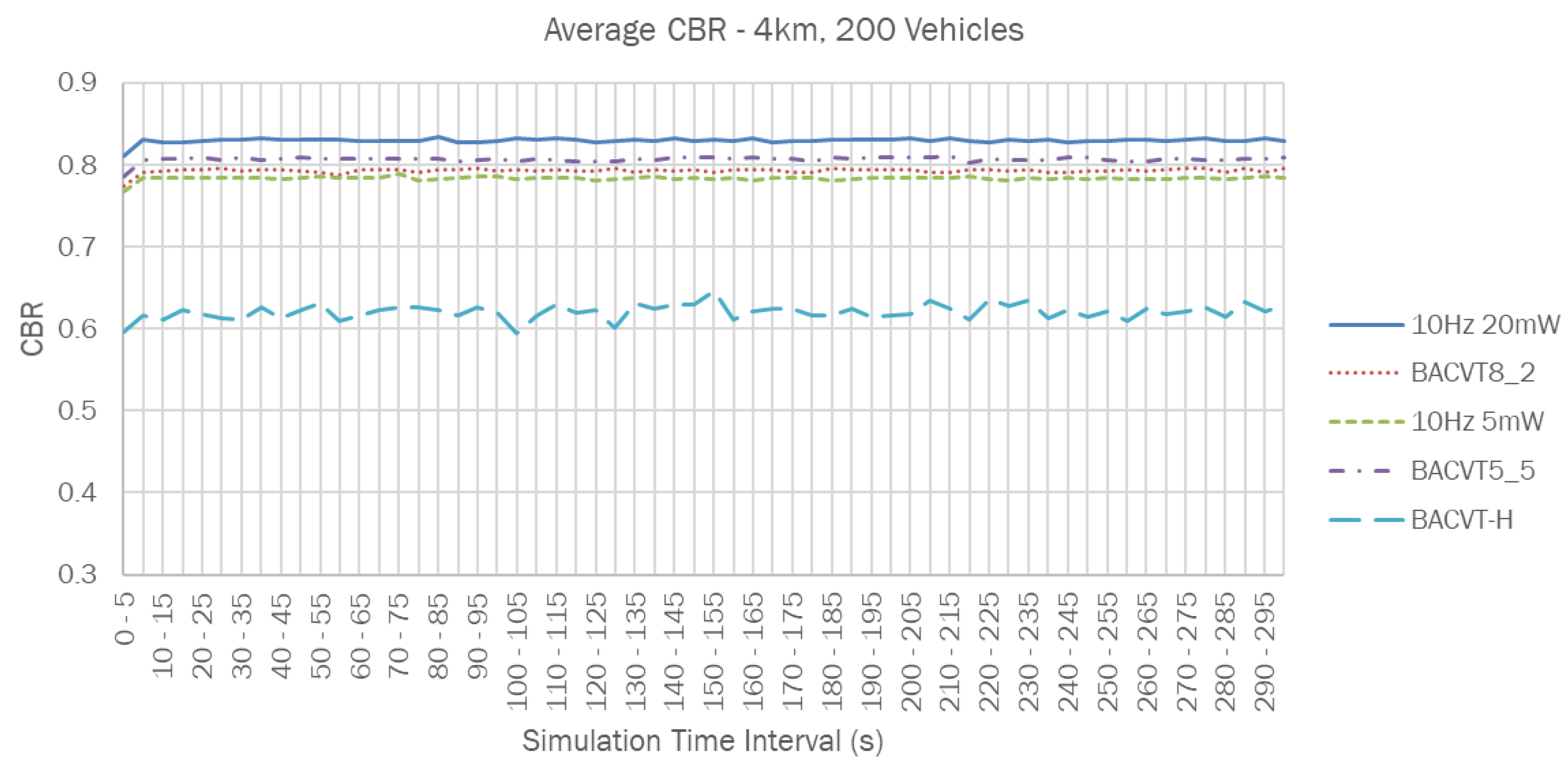
- 10 Hz 20 mW (All BSMs transmitted with 20 mW power);
- 10 Hz 5 mW (All BSMs transmitted with 5 mW power);
- BACVT8_2 (8 BSMs with Tx power = , 2 BSMs with Tx power = );
- BACVT5_5 (5 BSMs with Tx power = , 5 BSMs with Tx power = );
- BACVT-H (A hybrid approach combining BACVT with random rate control).
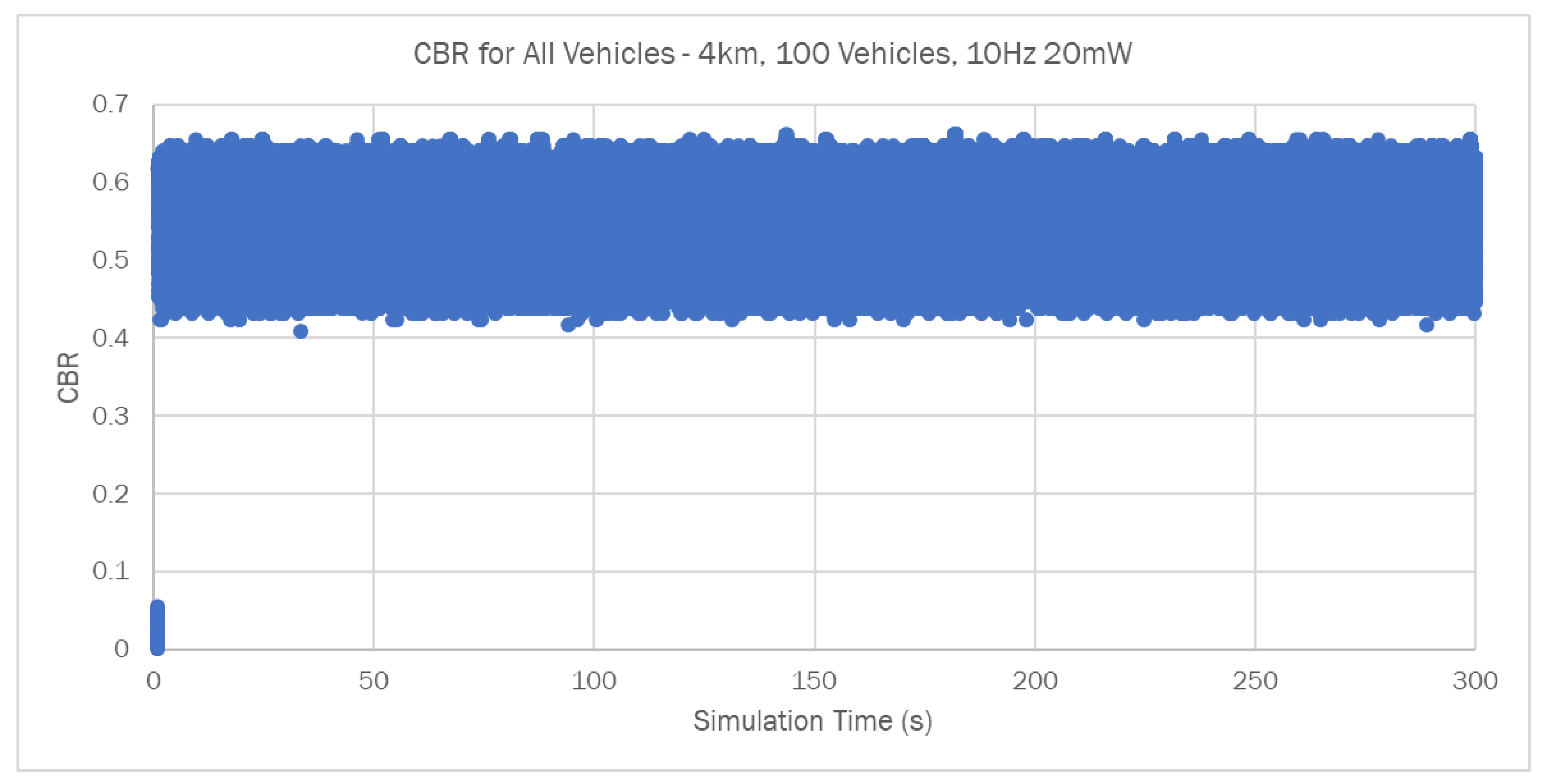
4.2. Average Channel Busy Ratio
4.3. Received BSMs over Different Distances
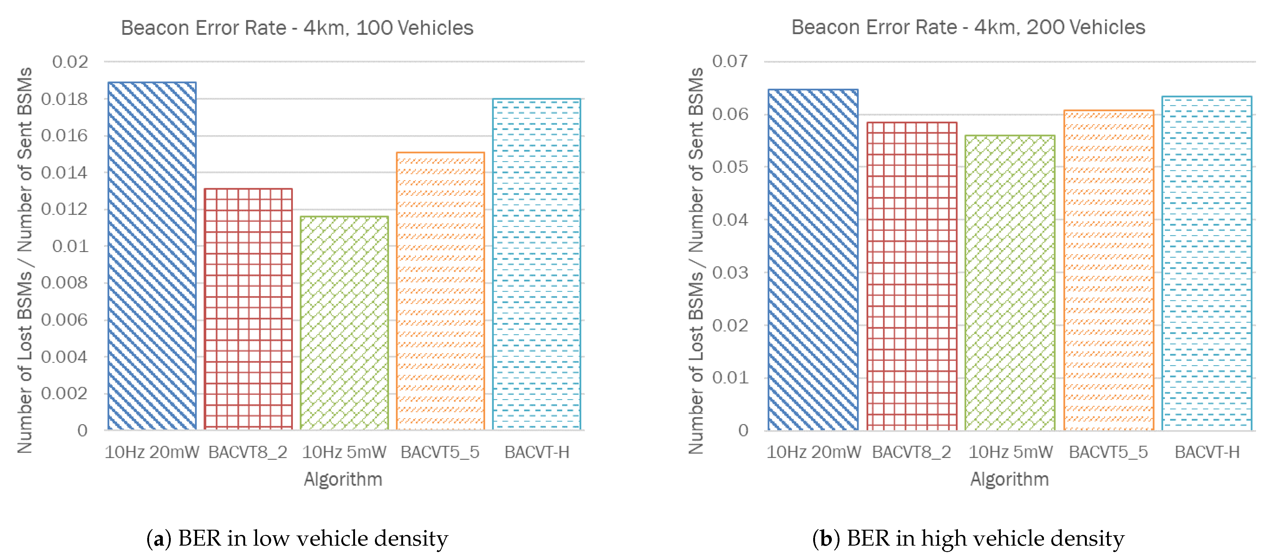
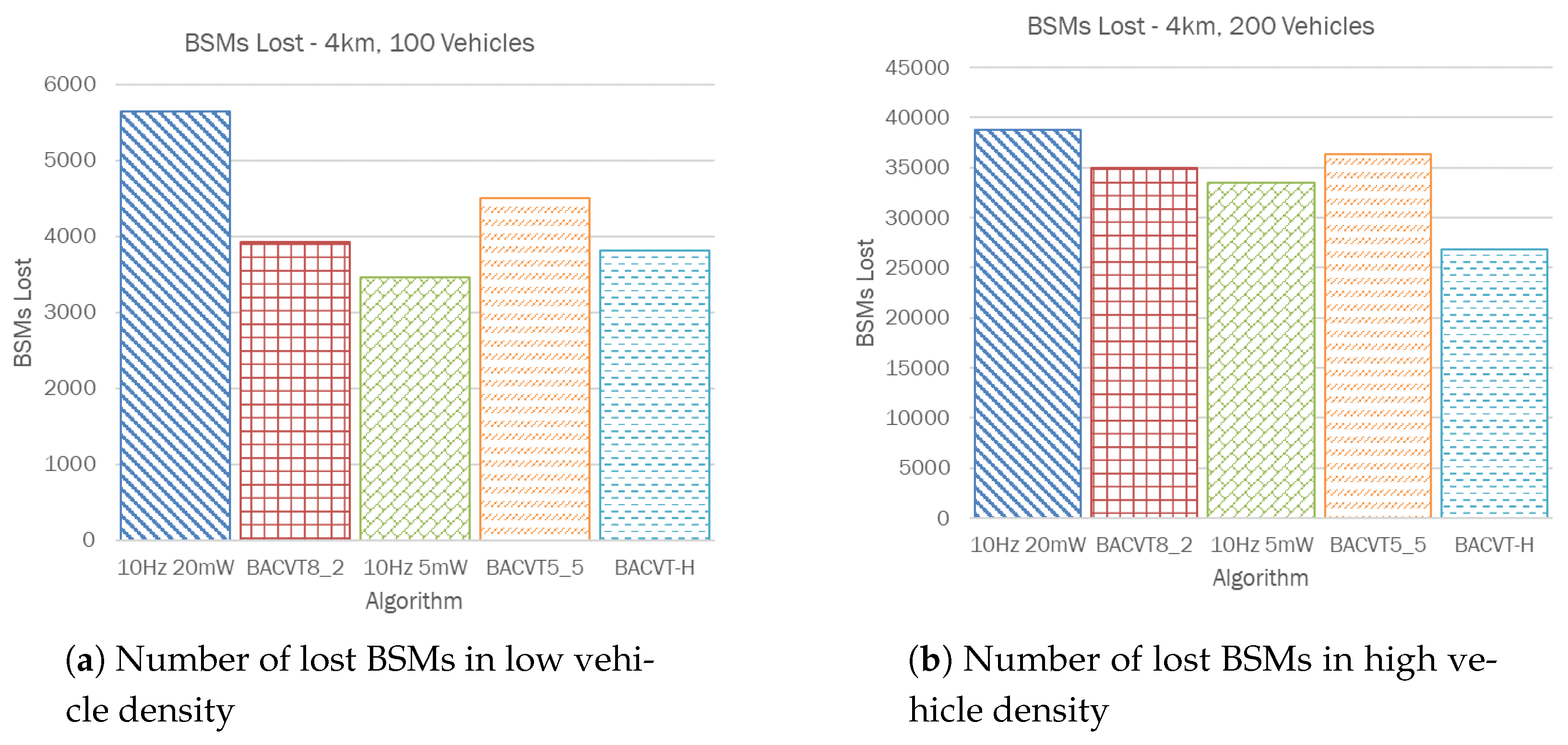
4.4. Beacon Error Rate
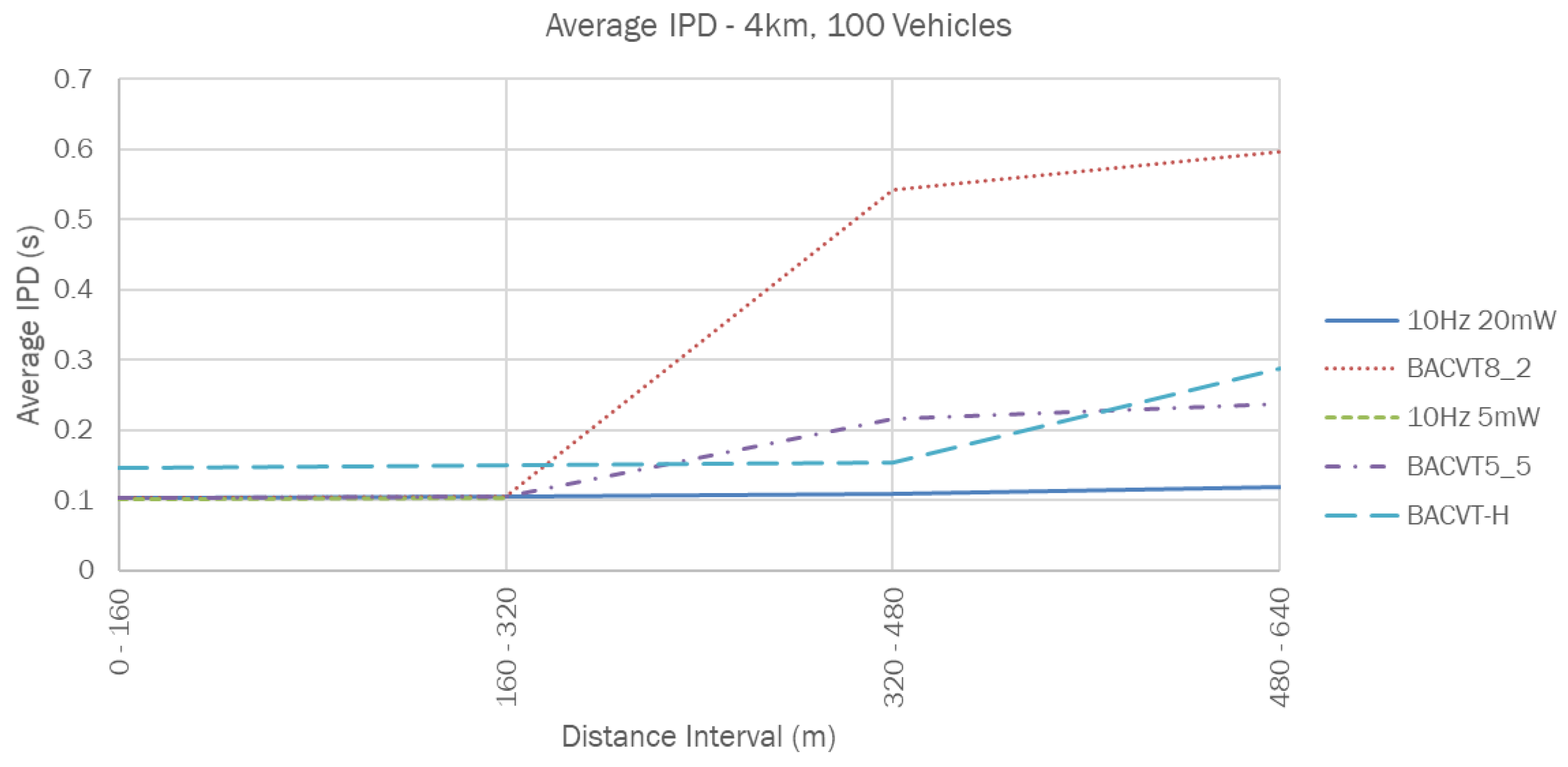
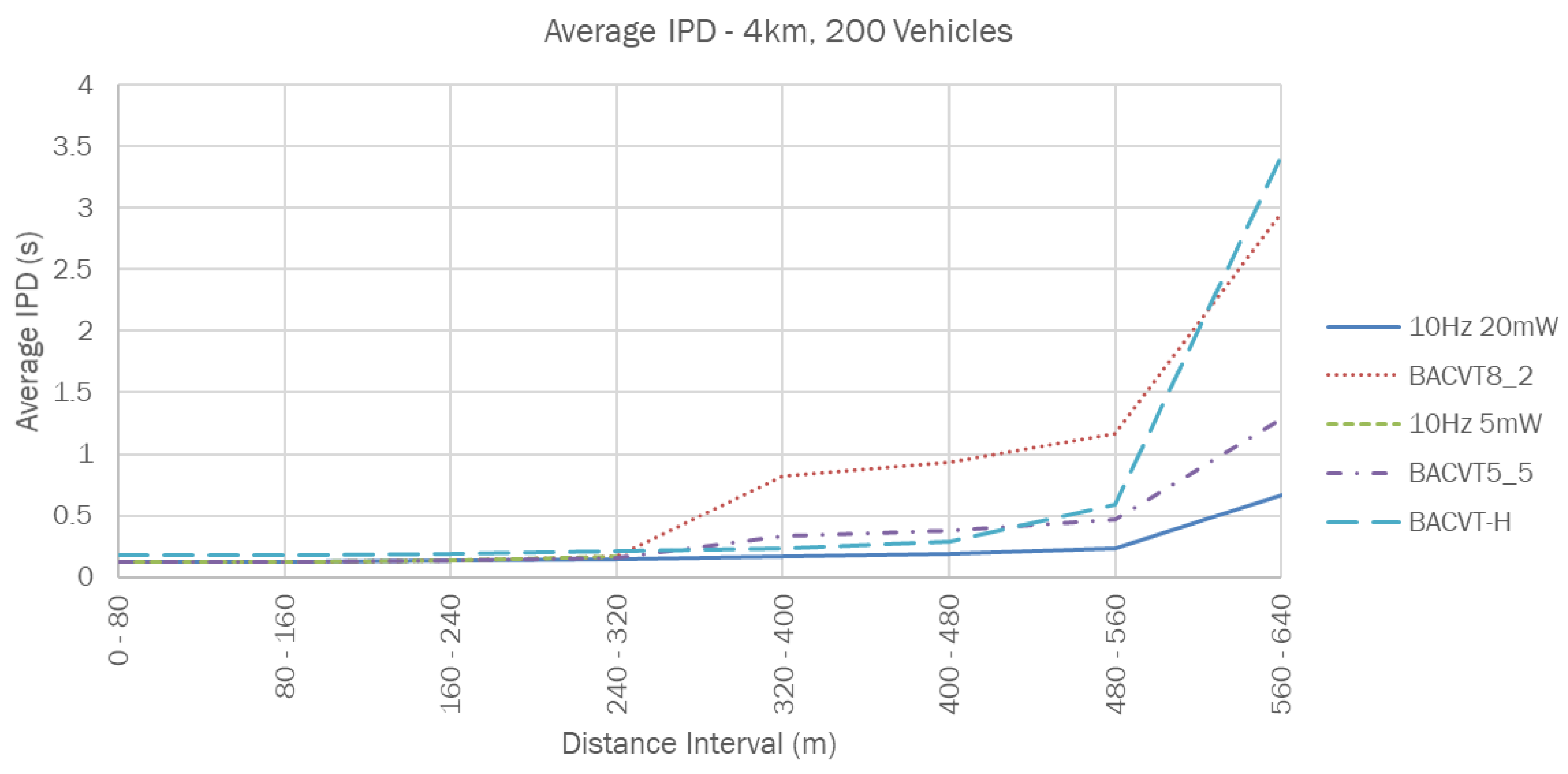
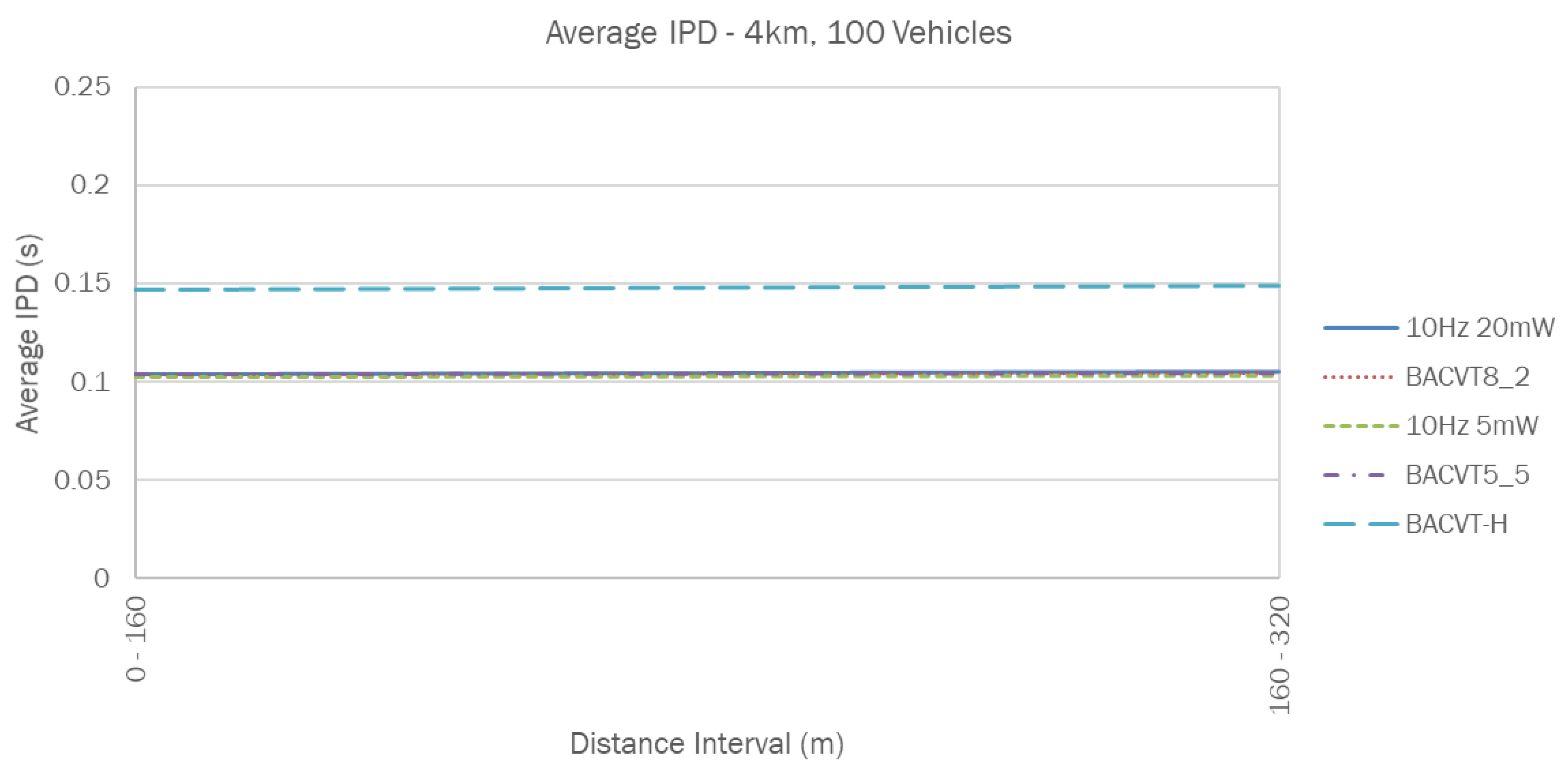
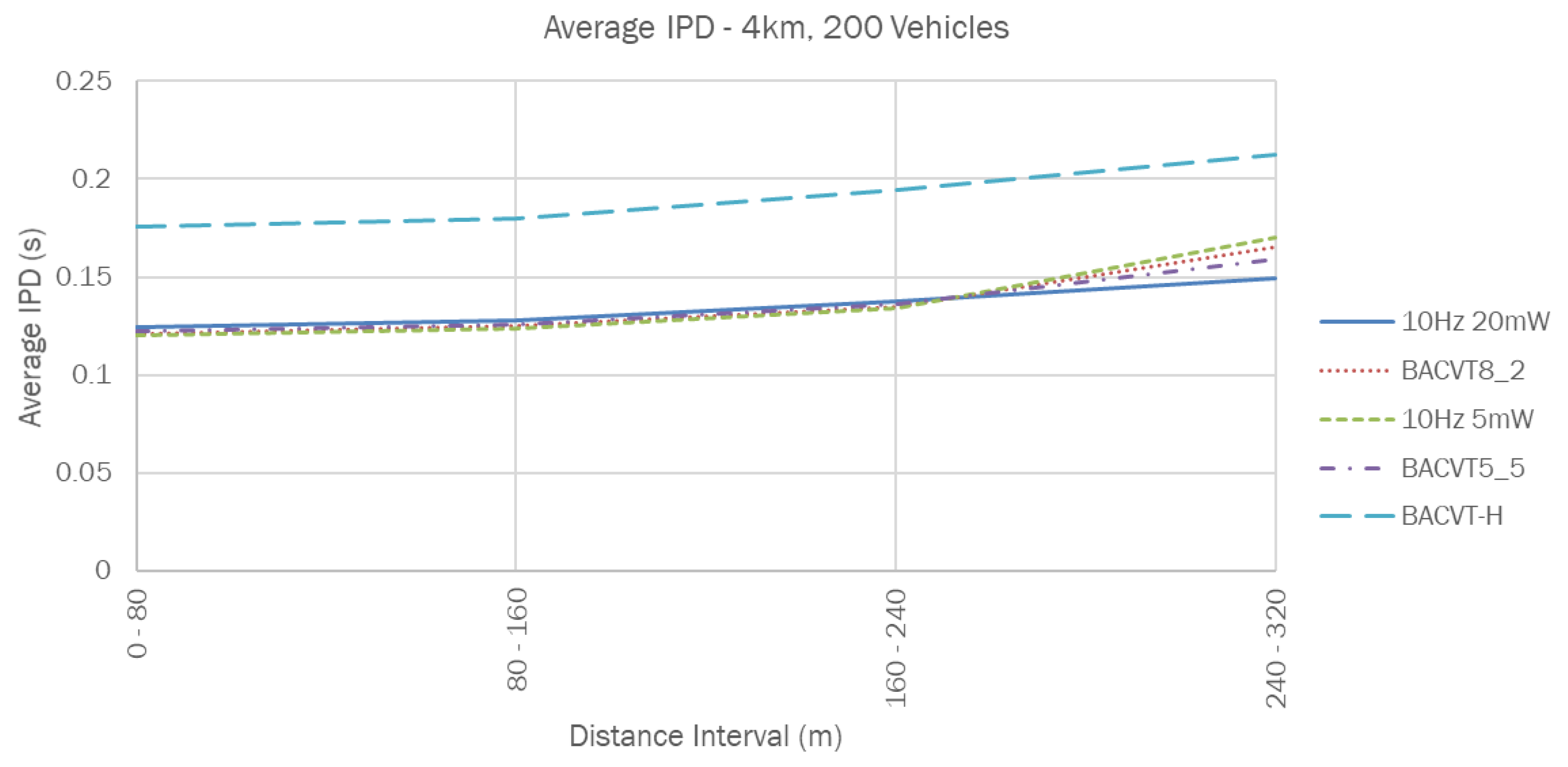
4.5. Inter-Packet Delay
5. Conclusions
Author Contributions
Funding
Data Availability Statement
Conflicts of Interest
References
- Harding, J.; Powell, G.; Yoon, R.; Fikentscher, J.; Doyle, C.; Sade, D.; Lukuc, M.; Simons, J.; Wang, J. Vehicle-to-Vehicle Communications: Readiness of V2V Technology for Application; Technical Report; United States National Highway Traffic Safety Administration: Washington, DC, USA, 2014.
- Car Crash Deaths and Rates. Available online: https://injuryfacts.nsc.org/motor-vehicle/historical-fatality-trends/deaths-and-rates/ (accessed on 6 June 2019).
- Toh, C. Ad Hoc Mobile Wireless Networks: Protocols and Systems; Pearson Education: England, UK, 2001. [Google Scholar]
- Li, Y. An Overview of the DSRC/WAVE Technology; Springer: New York, NY, USA, 2012; Volume 74. [Google Scholar]
- Kenney, J.B. Dedicated Short-Range Communications (DSRC) Standards in the United States. Proc. IEEE 2011, 99, 1162–1182. [Google Scholar] [CrossRef]
- Eggerton, J. FCC to Split up 5.9 GHZ. 2019. Available online: https://www.nexttv.com/news/fcc-to-split-up-5-9-ghz (accessed on 7 July 2021).
- SAE International. SAE J2735: Dedicated Short Range Communications (DSRC) Message Set Dictionary; Technical Report; SAE International: Warrendale, PA, USA, 2009. [Google Scholar]
- ETSI. ETSI (2013) ETSI EN 302 637-2 (V1.3.0) —Intelligent Transport Systems (ITS); Vehicular Communications; Basic Set of Applications; Part 2: Specification of Cooperative Awareness Basic Service; Technical Report; ETSI: Sophia Antipolis CEDEX, France, 2013. [Google Scholar]
- Bray, D.A. Modernizing the FCC’s IT; Federal Communications Commission Std.: Washington, DC, USA, 2015. [Google Scholar]
- Bansal, G.; Kenney, J.B.; Rohrs, C.E. LIMERIC: A linear adaptive message rate algorithm for DSRC congestion control. IEEE Trans. Veh. Technol. 2013, 62, 4182–4197. [Google Scholar] [CrossRef]
- Bilstrup, K.; Uhlemann, E.; Strom, E.G.; Bilstrup, U. Evaluation of the IEEE 802.11 p MAC method for vehicle-to-vehicle communication. In Proceedings of the 2008 IEEE 68th Vehicular Technology Conference, Calgary, AB, USA, 21–24 September 2008; pp. 1–5. [Google Scholar]
- Liu, X.; Jaekel, A. Congestion Control in V2V Safety Communication: Problem, Analysis, Approaches. Electronics 2019, 8, 540. [Google Scholar] [CrossRef]
- Bansal, G.; Lu, H.; Kenney, J.B.; Poellabauer, C. EMBARC: Error model based adaptive rate control for vehicle-to-vehicle communications. In Proceedings of the Tenth ACM International Workshop on Vehicular Inter-Networking, Systems, and Applications, Taipei, Taiwan, 25 June 2013; pp. 41–50. [Google Scholar]
- Ogura, K.; Katto, J.; Takai, M. BRAEVE: Stable and adaptive BSM rate control over IEEE802. 11p vehicular networks. In Proceedings of the 2013 IEEE 10th Consumer Communications and Networking Conference (CCNC), Las Vegas, NV, USA, 11–14 January 2013; pp. 745–748. [Google Scholar]
- Kloiber, B.; Härri, J.; Strang, T. Dice the TX power—Improving awareness quality in VANETs by random transmit power selection. In Proceedings of the 2012 IEEE Vehicular Networking Conference (VNC), Seoul, Korea, 14–16 November 2012; pp. 56–63. [Google Scholar]
- Torrent-Moreno, M.; Santi, P.; Hartenstein, H. Distributed fair transmit power adjustment for vehicular ad hoc networks. In Proceedings of the 2006 3rd Annual IEEE Communications Society on Sensor and Ad Hoc Communications and Networks, Reston, VA, USA, 25–28 September 2006; Volume 2, pp. 479–488. [Google Scholar]
- Wang, M.; Chen, T.; Du, F.; Wang, J.; Yin, G.; Zhang, Y. Research on adaptive beacon message transmission power in VANETs. J. Ambient. Intell. Humaniz. Comput. 2020. [Google Scholar] [CrossRef]
- Mittag, J.; Schmidt-Eisenlohr, F.; Killat, M.; Härri, J.; Hartenstein, H. Analysis and design of effective and low-overhead transmission power control for VANETs. In Proceedings of the Fifth ACM International Workshop on VehiculAr Inter-NETworking, San Francisco, CA, USA, 15 September 2008; pp. 39–48. [Google Scholar]
- Shah, S.A.A.; Ahmed, E.; Rodrigues, J.J.; Ali, I.; Noor, R.M. Shapely value perspective on adapting transmit power for periodic vehicular communications. IEEE Trans. Intell. Transp. Syst. 2018, 19, 977–986. [Google Scholar] [CrossRef]
- Kloiber, B.; Härri, J.; Strang, T.; Sand, S.; Garcia, C.R. Random transmit power control for DSRC and its application to cooperative safety. IEEE Trans. Dependable Secur. Comput. 2015, 13, 18–31. [Google Scholar] [CrossRef]
- Bansal, G.; Kenney, J.B. Achieving weighted-fairnessin message rate-based congestion control for DSRC systems. In Proceedings of the 2013 IEEE 5th International Symposium on Wireless Vehicular Communications (WiVeC), Dresden, Germany, 2–3 June 2013; pp. 1–5. [Google Scholar]
- Tielert, T.; Jiang, D.; Hartenstein, H.; Delgrossi, L. Joint power/rate congestion control optimizing packet reception in vehicle safety communications. In Proceedings of the Tenth ACM International Workshop on Vehicular Inter-Networking, Systems, and Applications, Taipei, Taiwan, 25 June 2013; pp. 51–60. [Google Scholar]
- Huang, C.L.; Fallah, Y.P.; Sengupta, R.; Krishnan, H. Adaptive intervehicle communication control for cooperative safety systems. IEEE Netw. 2010, 24, 6–13. [Google Scholar] [CrossRef]
- Math, C.B.; Ozgur, A.; de Groot, S.H.; Li, H. Data Rate based Congestion Control in V2V communication for traffic safety applications. In Proceedings of the 2015 IEEE Symposium on Communications and Vehicular Technology in the Benelux (SCVT), Luxembourg, 24 November 2015; pp. 1–6. [Google Scholar]
- Schmidt, R.K.; Brakemeier, A.; Leinmüller, T.; Kargl, F.; Schäfer, G. Advanced carrier sensing to resolve local channel congestion. In Proceedings of the Eighth ACM International Workshop on Vehicular Inter-Networking, Las Vegas, NV, USA, 23 September 2011; pp. 11–20. [Google Scholar]
- Sharmaa, R.; CSb, L.; VSc, R. Congestion control mechanisms to avoid congestion in VANET: A comparative review. In Artificial Intelligence and Speech Technology, Proceedings of the 2nd International Conference on Artificial Intelligence and Speech Technology,(AIST2020), Delhi, India, 19–20 November 2020; CRC Press: Nottingham, UK, 2021; p. 453. [Google Scholar]
- Wang, J.; Jiang, C.; Zhang, K.; Quek, T.Q.; Ren, Y.; Hanzo, L. Vehicular sensing networks in a smart city: Principles, technologies and applications. IEEE Wirel. Commun. 2017, 25, 122–132. [Google Scholar] [CrossRef]
- Wang, J.; Jiang, C.; Han, Z.; Ren, Y.; Hanzo, L. Internet of vehicles: Sensing-aided transportation information collection and diffusion. IEEE Trans. Veh. Technol. 2018, 67, 3813–3825. [Google Scholar] [CrossRef]
- Boban, M. ECPR: Environment-and Context-Aware DCC Algorithm’; NEC Laboratories Europe: Heidelberg, Germany, 2015. [Google Scholar]
- Bansal, G.; Cheng, B.; Rostami, A.; Sjoberg, K.; Kenney, J.B.; Gruteser, M. Comparing LIMERIC and DCC approaches for VANET channel congestion control. In Proceedings of the 2014 IEEE 6th International Symposium on Wireless Vehicular Communications (WiVeC 2014), Vancouver, BC, Canada, 14–15 September 2014; pp. 1–7. [Google Scholar]
- Sepulcre, M.; Gozalvez, J.; Altintas, O.; Kremo, H. Adaptive beaconing for congestion and awareness control in vehicular networks. In Proceedings of the 2014 IEEE Vehicular Networking Conference (VNC), Paderborn, Germany, 3–5 December 2014; pp. 81–88. [Google Scholar]
- Aygun, B.; Boban, M.; Wyglinski, A.M. ECPR: Environment-and context-aware combined power and rate distributed congestion control for vehicular communications. Comput. Commun. 2016, 93, 3–16. [Google Scholar] [CrossRef][Green Version]
- Goudarzi, F.; Asgari, H. Non-cooperative beacon power control for VANETs. IEEE Trans. Intell. Transp. Syst. 2018, 20, 777–782. [Google Scholar] [CrossRef]
- Joseph, M.; Liu, X.; Jaekel, A. An adaptive power level control algorithm for DSRC congestion control. In Proceedings of the 8th ACM Symposium on Design and Analysis of Intelligent Vehicular Networks and Applications, Montreal, QC, Canada, 28 October–2 November 2018; pp. 57–62. [Google Scholar]
- Willis, J.T.; Jaekel, A.; Saini, I. Decentralized congestion control algorithm for vehicular networks using oscillating transmission power. In Proceedings of the 2017 Wireless Telecommunications Symposium (WTS), Chicago, IL, USA, 26–28 April 2017; pp. 1–5. [Google Scholar]
- Sommer, C.; German, R.; Dressler, F. Bidirectionally coupled network and road traffic simulation for improved IVC analysis. IEEE Trans. Mob. Comput. 2010, 10, 3–15. [Google Scholar] [CrossRef]
- Varga, A.; Hornig, R. An overview of the OMNeT++ simulation environment. In Proceedings of the 1st International Conference on Simulation Tools and Techniques for Communications, Networks and Systems & Workshops, Marseille, France, 3–7 March 2008; ICST (Institute for Computer Sciences, Social-Informatics and Telecommunications Engineering: Brussels, Belgium, 2008; p. 60. [Google Scholar]
- Behrisch, M.; Bieker, L.; Erdmann, J.; Krajzewicz, D. SUMO–simulation of urban mobility: An overview. In Proceedings of the Third International Conference on Advances in System Simulation, Barcelona, Spain, 23–29 October 2011. [Google Scholar]


| Distance (m) | Sent BSMs | 10 Hz 20 mW | 10 Hz 5mW | ||
|---|---|---|---|---|---|
| Received BSMs | Lost BSMs | Received BSMs | Lost BSMs | ||
| 50 | 5982 | 5980 | 2 | 5980 | 2 |
| 100 | 5982 | 5980 | 2 | 5980 | 2 |
| 150 | 5982 | 5980 | 2 | 5980 | 2 |
| 200 | 5982 | 5980 | 2 | 5980 | 2 |
| 250 | 5982 | 5980 | 2 | 5969 | 13 |
| 300 | 5982 | 5980 | 2 | 2872 | 3110 |
| 350 | 5982 | 5980 | 2 | 0 | 5982 |
| 400 | 5982 | 5980 | 2 | 0 | 5982 |
| 450 | 5982 | 5978 | 4 | 0 | 5982 |
| 500 | 5982 | 5957 | 25 | 0 | 5982 |
| 550 | 5982 | 5481 | 501 | 0 | 5982 |
| 600 | 5982 | 1728 | 4254 | 0 | 5982 |
| 650 | 5982 | 0 | 5982 | 0 | 5982 |
| 700 | 5982 | 0 | 5982 | 0 | 5982 |
| Name | Value |
|---|---|
| Default Beacon Rate | 10 BSMs |
| Random Beacon Rate | 5–10 BSMs |
| BSM Size | 512 Bytes |
| Transmission Power for Far Range | 20 mW |
| Transmission Power for Near Range | 5 mW |
| Data Rate | 6 Mbps |
| Min. Power Level | −110 dBm |
| Noise Floor | −98 dBm |
| High Vehicle Density | 50 Vehicles/km |
| Low Vehicle Density | 25 Vehicles/km |
| Highway Length/Lanes | 4 km/4 |
| Simulation Time | 300 s |
| Received BSMs—4 km, 100 Vehicles | |||||
|---|---|---|---|---|---|
| Distance (m) | 10 Hz 20 mW | 10 Hz 5 mW | BACVT8_2 | BACVT5_5 | BACVT-H |
| x ≤ 100 | 840,606 | 845,217 | 844,049 | 843,161 | 595,147 |
| 100 < x ≤ 300 | 2,178,771 | 2,202,846 | 2,196,500 | 2,191,305 | 1,542,993 |
| x > 300 | 3,760,760 | 0 | 750,529 | 1,879,596 | 2,142,281 |
| Received BSMs–4 km, 200 Vehicles | |||||
|---|---|---|---|---|---|
| Distance (m) | 10 Hz 20 mW | 10 Hz 5 mW | BACVT8_2 | BACVT5_5 | BACVT-H |
| x ≤ 100 | 5,091,994 | 5,249,359 | 5,218,042 | 5,174,255 | 3,612,076 |
| 100 < x ≤ 300 | 6,346,860 | 6,056,645 | 6,116,713 | 6,208,877 | 4,477,210 |
| x > 300 | 7,328,452 | 0 | 1,465,741 | 3,663,096 | 4,153,365 |
Publisher’s Note: MDPI stays neutral with regard to jurisdictional claims in published maps and institutional affiliations. |
© 2021 by the authors. Licensee MDPI, Basel, Switzerland. This article is an open access article distributed under the terms and conditions of the Creative Commons Attribution (CC BY) license (https://creativecommons.org/licenses/by/4.0/).
Share and Cite
Liu, X.; St. Amour, B.; Jaekel, A. Balancing Awareness and Congestion in Vehicular Networks Using Variable Transmission Power. Electronics 2021, 10, 1902. https://doi.org/10.3390/electronics10161902
Liu X, St. Amour B, Jaekel A. Balancing Awareness and Congestion in Vehicular Networks Using Variable Transmission Power. Electronics. 2021; 10(16):1902. https://doi.org/10.3390/electronics10161902
Chicago/Turabian StyleLiu, Xiaofeng, Ben St. Amour, and Arunita Jaekel. 2021. "Balancing Awareness and Congestion in Vehicular Networks Using Variable Transmission Power" Electronics 10, no. 16: 1902. https://doi.org/10.3390/electronics10161902
APA StyleLiu, X., St. Amour, B., & Jaekel, A. (2021). Balancing Awareness and Congestion in Vehicular Networks Using Variable Transmission Power. Electronics, 10(16), 1902. https://doi.org/10.3390/electronics10161902