Article

An Efficient Hardware Design for a Low-Latency Traffic Flow Prediction System Using an Online Neural Network

by
Yasmin Adel Hanafy
1,
Maggie Mashaly
1 and
Mohamed A. Abd El Ghany
1,2,*
1
Department of Information Engineering and Technology, German University in Cairo, New Cairo, Egypt
2
Technische Universität Darmstadt, 64289 Darmstadt, Germany
*
Author to whom correspondence should be addressed.
Electronics 2021, 10(16), 1875; https://doi.org/10.3390/electronics10161875
Submission received: 2 July 2021 / Revised: 27 July 2021 / Accepted: 29 July 2021 / Published: 4 August 2021
(This article belongs to the Section Artificial Intelligence Circuits and Systems (AICAS))

Abstract

:
Neural networks are computing systems inspired by the biological neural networks in human brains. They are trained in a batch learning mode; hence, the whole training data should be ready before the training task. However, this is not applicable for many real-time applications where data arrive sequentially such as online topic-detection in social communities, traffic flow prediction, etc. In this paper, an efficient hardware implementation of a low-latency online neural network system is proposed for a traffic flow prediction application. The proposed model is implemented with different Machine Learning (ML) algorithms to predict the traffic flow with high accuracy where the Hedge Backpropagation (HBP) model achieves the least mean absolute error (MAE) of 0.001. The proposed system is implemented using floating point and fixed point arithmetics on Field Programmable Gate Array (FPGA) part of the ZedBoard. The implementation is provided using BRAM architecture and distributed memory in FPGA in order to achieve the best trade-off between latency, the consumption of area, and power. Using the fixed point approach, the prediction times using the distributed memory and BRAM architectures are 150 ns and 420 ns, respectively. The area delay product (ADP) of the proposed system is reduced by 17 × compared with the hardware implementation of the latest proposed system in the literature. The execution time of the proposed hardware system is improved by 200 × compared with the software implemented on a dual core Intel i7-7500U CPU at 2.9 GHz. Consequently, the proposed hardware model is faster than the software model and more suitable for time-critical online machine learning models.

1. Introduction

The use of neural networks in various fields has been on the rise due to their ability to model nonlinear complex problems for solving classification and regression problems. The increase in development and advancement in neural networks have led them to be used in every aspect of human life like video surveillance [1], speech recognition [2], health care [3], intelligent transportation [4], weather forecasting and natural disasters monitoring [5], e-marketing [6], article analysis [7], and the oil and gas industry [8]. Numerous challenges are faced while building neural network models such as diminishing feature reuse [9], vanishing gradient [10], internal covariate shift during training [11], and saddle points [12] along with the need for huge of computational resources due to the large volume of training data. Researchers trying to address and solve these problems assume that neural network models are trained in batch learning mode, which needs the whole dataset to be available prior to training. This is not the case for streaming data, which is a continuous flow of data that requires being processed in real time without the need for data to be in the batch form. A lot of applications make use of streaming data such as traffic flow prediction, fraud detection, marketing, sales, and business analytics. Consequently, there is a tremendous importance for developing neural network models for streaming data [13].
Numerous attempts have been made in the literature to build online neural network models [14,15,16,17,18]. All of the work proposed is software-optimized and lacks the benefits of parallel processing hardware solutions found in FPGAs. Hardware Intellectual Property (IP) accelerators implemented on FPGAs can provide a quick response time, high performance, low power, high reliability, and flexibility for embedded applications, which makes them possible good options to be used instead of GPUs, which consume more power than FPGAs.
One of the areas where online neural networks can make a high impact is traffic flow prediction, which is one of the top fields that are investigated in Intelligent Transport Systems (ITS). Not only does it assists travelers in making suitable travel decision but also it is helpful in autonomous vehicles to reduce traffic congestion and car accidents [19]. Traffic flow prediction relies heavily on historical and real-time traffic data gathered from different sensor sources; radars, including inductive loops; mobile phones; global positioning systems; cameras; crowd sourcing; social media; etc. The traffic data vary within time because of the extensive widespread traditional traffic sensors and new traffic sensor technologies appearing. Consequently, traffic flow prediction is a very suitable case study to test the efficiency of an online neural network model.
In this paper, an adequate online machine learning model is presented for traffic flow prediction that provides highly accurate results. In addition, the inference part was implemented on the hardware by extracting the weights after training. The results show that the speed of the hardware design is much faster than that of software. Therefore, it is better to use hardware models for time-critical online machine learning algorithms. This paper investigates three different hardware architectures for storing the weights: are Block RAM (BRAM), Double Data Rate (DDR), and distributed memory to find the most suitable hardware design that is adequate for online machine learning. The implementation using floating point and fixed point arithmetics on Field Programmable Gate Array (FPGA) is investigated in order to achieve the best trade-off between latency, the consumption of area, and power.
The rest of the paper is organized as follows: Section 2 presents the related work. Section 3 provides the background for machine learning models used in the paper to compare the Online Neural Network (ONN) model using Hedge Back Propagation (HBP). Section 4 provides the background on Adaptive Momentum (ADAM) optimizer. Section 5 provides the background on the ONN using HBP algorithm. Section 6 provides a detailed description of the proposed hardware architecture of the ONN accelerator. Section 7 evaluates and compares the performance of the six hardware implementations. Section 8 discusses the conclusions drawn from the paper. Finally, future work is presented in Section 9.

2. Related Work

2.1. Software Implementation of Online Neural Networks

Due to the importance of traffic flow prediction and the need for traffic management, many researchers are developing machine learning models for traffic flow prediction. Most significant parts of this work discussed in this section. In [20], a convolution neural network (CNN) model is implemented to predict traffic flow. Since CNN is mainly used for images, the spatiotemporal traffic dynamics are converted to images. These images are composed of 2D time–space matrices that shows the relation between time and space of traffic flow. However, this method is very complex and time-consuming for converting spatiotemporal traffic dynamics to images. The Stacked Autoencoder (SAE) model for traffic flow prediction was implemented in [21,22,23] to enhance feature extraction. On the other hand, one of the main disadvantages of SAEs is that they do not produce significant effect when errors are present in the first layers [24]. Consequently, their usage is not preferred for traffic flow prediction. A comparison among different ensemble decision trees models, which are Gradient Boosting Regression Tress (GBRT), Random Forest (RF), and Extreme Gradient Boosting (XGBoost), was conducted in [25]. Ensemble models were used to increase the performance of decision tree by combining multiple weak learners to produce a strong learner that can provide more accurate predictions. There are two problems discussed in the paper that may appear in traffic flow prediction problems. The first problem is that predicting traffic flow is a dynamic nonlinear problem due to extraordinary events, such as accidents and congestion. The second problem is that scalable models are needed to efficiently handle large amount of data. A nonlinear dataset, published by VicRoads for the state of Victoria, Australia, was used to overcome the first problem. Finally, XGBoost, which is a scalable learning system, performed the best in terms of accuracy and time complexity as it achieved a mean absolute error of 0.6283. However, this error was obtained by training on a small number of samples.
The authors of [26] proposed a short-term traffic prediction model using back propagation artificial NN for two-lane highways with mixed traffic in India. They used Tanh and sigmoid activation functions, which need high computation time. Additionally, Reference [27] used Support Vector Regression (SVR), RF, Neural Networks (NN), and Multiple Linear Regression (MLR) to predict traffic status in the city of Thessaloniki. The mean absolute errors obtained were 3.67 for SVR, 3.74 for MLP, 3.87 for RF, and 4.1 for MLR; but these errors are not adequate to solve the traffic flow prediction problem.
Furthermore, multiple regression models for traffic flow prediction, which are MLR and RF were implemented in [28]. Then, these algorithms’ results were compared with SVR and artificial NN. The lowest root mean square errors obtained from the GPS truck trajectory dataset were 19.06 for MLR and 20.97 for RF. References [29,30,31,32] proposed deep architectures; however, deep networks are considered inefficient solutions for real-time applications as they result in high computational time. Reference [29] implemented a deep belief network (DBN) at the bottom and a multitask regression layer (MTL) at the top to solve the traffic flow prediction problem in transportation modelling and management. It used the PeMs dataset with a low prediction accuracy of 90%. On the contrary, Reference [30] implemented STResNet to predict the inflow and outflow of crowds in each region of a city. The model was based on a convolution neural network. They used two different datasets: TaxiBJ and Trajectory data, which are the taxicab GPS data and meteorology data in Beijing. The RMSE for the two datasets were 16.96 and 6.93, respectively.
Diffusion Convolutional Recurrent Neural Network (DCRNN) for traffic forecasting was proposed by [32]. The dataset was PEMS-BAY, which is collected by California Transportation Agencies (CalTrans) Performance Measurement System (PeMS), obtaining an MAE of 2.07. Furthermore, Long Short-Term Memory (LSTM) for traffic flow prediction was implemented by [33]. It used data of a toll station in Xi’an and produced an MAE equal to 20.156.
There are several attempts to design online learning algorithms. They are explained in this section. First was to discuss is the work by [34], which was able to overcome catastrophic forgetting; however, the model is complex since new units are added with each new available example. Online kernel classification models were designed by [35,36]. Although these models learn nonlinearity, they suffer from shallow networks. In [35], the final prediction is determined from some previous predefined kernels in an online learning fashion. Their work is related to online predictions with expert advice using Hedge algorithm. They proposed two different approaches to update the kernels, which are deterministic and stochastic. The stochastic approach has some limitations such as having difficulty in choosing the type of kernel for the best accuracy and they are not able to learn a feature representation. A Cost-Sensitive Online Multiple Kernel Classification algorithm was proposed by [36]. Although the model does not need to define a prior kernel, with the increased number of features, the model slowly converges for a small number of instances. Finally, a deep network model was designed by [16,37,38]. However, they are not appropriate for streaming data applications because they use sliding window approach with a (mini) batch training.

2.2. Hardware Implementation of Neural Networks

Implementing hardware neural network is favorable compared with the software implementation since hardware achieves low latency and low power consumption. Not only do NN designers face challenges in implementing efficient real-time NN models but also they have to deal with an immense number of multiplication, addition, and sequential programming, which is always a bottleneck, especially for ONN. Consequently, designers turn to hardware implementation for NN. Nowadays, advanced FPGAs have specialized blocks such as DSP and BRAM to conduct complicated mathematical operations. Hence, FPGAs are now extremely adequate for real-time applications [39]. Although there are many approaches for implementing hardware neural network accelerators on FPGA boards, none of them support an online neural network architecture. The state-of-the-art in this research area is discussed in this subsection. Reference [40] has implemented a multi-layer perceptron neural network using VHDL, ModelSim SE, and floating point arithmetic operations. It designed an on-chip Multilayer Perceptron (MLP) with Back Propagation algorithm. The MLP was used to solve the XOR problem using VHDL and tested on Virtex-E board. The sigmoid activation function package was used for implementation of the XOR. The model operated at a low frequency equal to 5.332 MHz and used 87% of LUT and 98% of slices.
A hardware Multilayer Perceptron (MLP) for Real-Time Human Activity Classification was implemented by [41]. The paper only implemented the prediction phase on hardware using an Artix-7 board. All weights were stored in the board’s on-chip memory instead of an off-chip memory to reduce the communication latency. Consequently, it supports offline training, which represents one of the main disadvantages in this model, since it has to be reprogrammed each time there are new weights available. Additionally, hardware Multi-Layer perceptron for speech recognition on a Virtex-E board was implemented by [42]. The hardware model was only designed for the classification phase. Similar to [41], the weights were stored in Virtex-E board’s on-chip RAM. Hence, it has the same disadvantage. In addition, Reference [43] designed wearable human activity recognition (HAR) systems on Spartan-6 LX family devices. The design allocated relatively high resources compared with other implementations that exploit less number of resources; 5432 LUT, 65 BRAM, and 19 DSPs.
The research work conducted in various studies as in [44,45,46,47] implemented a Multi-Layer neural network using fixed point arithmetic. Reference [44] was implemented on a Virtex-4 FPGA. It was shown that a network with 1500 neurons and 32 layers made use of 50% of the resources of the board. References [45,46] implemented a two-layer model. Reference [45] implemented a full parallel and pipelined (32-3-4) neural network topology with 8 bit fixed points. It was implemented on Xilinx Virtex-6 and Virtex-7 boards. It was able to classify 288 pixels in 0.67 μ s. The design used less than 4% of board resources. It occupied 2798 LUT, 7 RAM18E1, and 12 DSPs. Contrarily, Reference [46] implemented a parallel neural network topology for gas classification. The model presented obtained an accuracy of 97.4% and a latency of 540 ns. Additionaly, it was implemented on Zynq-7000 XC7Z010T-1CLG400 from Xilinx. Finally, [47] implemented a five-layer multilayer perceptron suitable for chaotic time series prediction. It used hyperbolic tangent activation function that consumed a lot of hardware resources. References [48,49,50,51] implemented a three-layer Artificial Neural Network (ANN). They all used a sigmoid activation function, which consumes lots of resources and takes huge computation times. Moreover, they used a distributed memory for storing weights which is not applicable for online applications. Finally, Reference [50] only simulated the ANN without testing it on a real FPGA.

3. Adopted Machine Learning Models

The machine learning models used to compare the performance of the implemented online neural network are explained in this section.

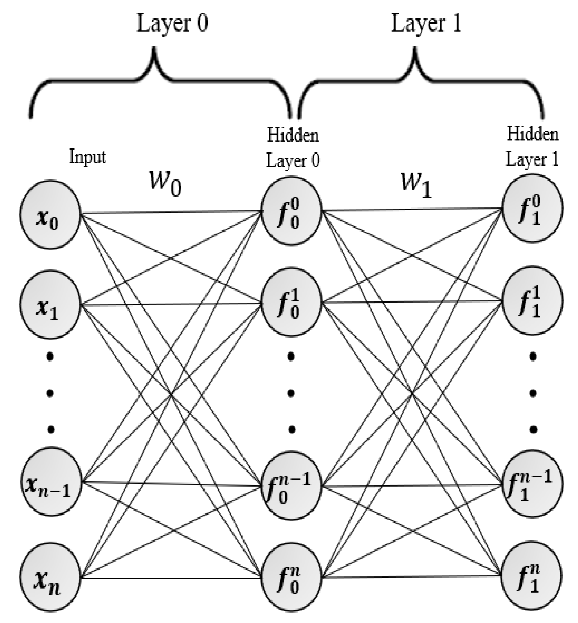
3.1. Multi-Layer Perceptron (MLP)

Neural Networks are modeled as collections of neurons that are connected in a definite graph. The outputs of neurons are inputs to other neurons in the following layer. Neural Network models are organized into definite layers of neurons. Commonly, a fully connected layer is used for Multi-Layer Preceptron, in which neurons between two adjacent layers are fully connected but neurons within a single layer are not connected. Figure 1 is a generic shape of an MLP. In order to produce nonlinearity, activation functions such as Rectified linear unit (Relu), sigmoid, Tanh, etc. are added to the hidden layers. On the other hand, the output layer neurons commonly do not have an activation function. The reason is that the last output layer is usually taken to represent either the class scores (e.g., in classification), which are normally real-valued numbers, or some kind of real-valued target (e.g., in regression). The formulas for MLP are as follows:
f ( 0 ) = σ ( W ( 0 ) x + b ( 0 ) )
f ( l ) = σ ( W ( l ) f ( l 1 ) + b ( l ) ) L = 1 , . . . , L 1
f ( L ) = W ( L ) f ( L 1 ) + b ( L )

3.2. Multiple Linear Regression (MLR)

Linear regression (LR) is a supervised learning algorithm that uses a parametric linear function for a regression problem. It is used to predict a dependent variable (output) from independent variables (input). The formula for MLR is as follows:
y i = β 0 + β 1 x i 1 + β 2 x i 2 + β 3 x i 3 + . . . . . + β p x i n
where i = n samples, x i 1 , x i 2 , x i 3 . . . . x i n present the independent variables (input), and y i is the dependent variable (output). The β coefficients denote the slope for each independent variable. It is calculated as follows:
β = ( X T . X ) 1 ( X T . Y )
Although MLR is considered the simplest algorithm for ML algorithms, it represents an accurate model for linear regression [52].

4. Adaptive Momentum (ADAM)

Optimization has been rapidly revolutionized with the increased development in machine learning techniques. Choosing an appropriate optimizer affects both the timing and accuracy for a ML model. The ADAM [53] optimizer is an adaptive optimization algorithm developed for deep neural networks. The optimizer is powerful in accelerating the training process by generating adaptive learning rates and is a combination of both SGD with momentum and RMSprop algorithms. That is why an ADAM optimizer is used in the MLP implemented in this thesis. The following equations show how ADAM works: Equation (6) is the gradient on a current mini-batch.
g t = f ( w )
Equations (7) and (8) are two moments. Betas are considered exponential decay rates, which are hyperparameters for the moment estimate. The first moment is the mean while the second moment is uncentered variance, β 1 is 0.9, and β 2 is 0.999.
m t = β 1 m t 1 + ( 1 β 1 ) g t
v t = β 2 v t 1 + ( 1 β 2 ) g t 2
It is clear that the similarities appear in the folloiwng:
  • m is the exponential moving average of gradients (such as in SGD with momentum) (Equation (7)).
  • The learning rate α is divided by square root of v, which is the exponential moving average of squared gradients (suhc as in RMSprop) (Equation (8)).
The next two equations are the bias correction.
m t = m t 1 β 1 t
v t = v t 1 β 2 t
Finally, the weights are updated using the bias correction equations and η which is the step size.
w t = w t 1 η m t v t + ε

5. Online Neural Network (ONN) Model

Online learning has no separation phase between training and testing. Each time an example is passed to the model, it is first considered as a test example, and the model should predict an output. Then, after the true value is passed, the same example can be used as a training example to improve the model in prediction. Moreover, online learning is known as learning a hypothesis from data examples sequentially, one at a time [54]. In this section, the inference and the training parts of the online machine learning are explained.

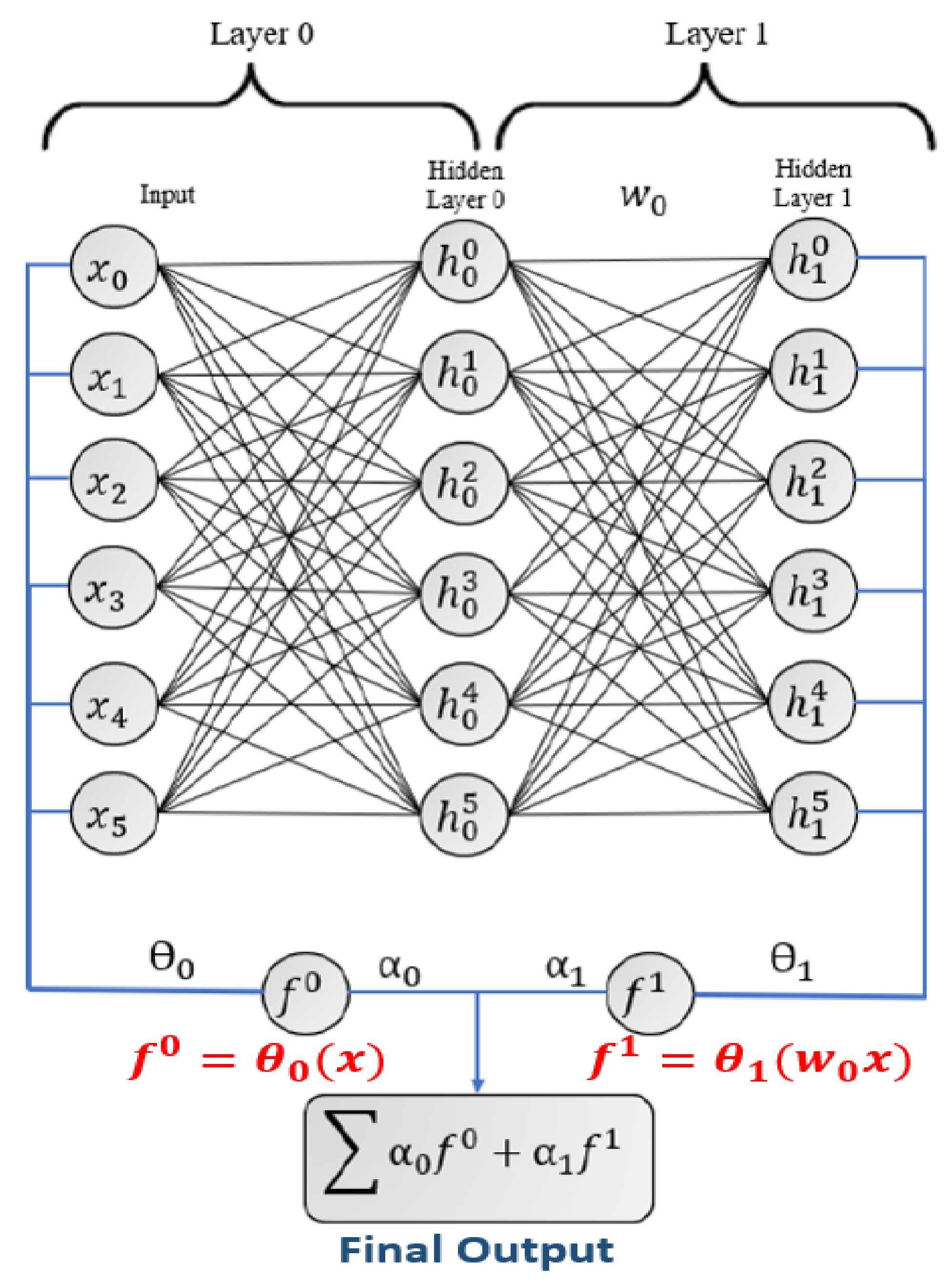
5.1. Hedge Backpropagation (HBP) Prediction

In this section, the prediction of an online Neural Network using Hedge Backpropagation [14] is explained for a network with L hidden layers. HBP predicts the final output from a weighed combination of classifiers denoted by α ( l ) f ( l ) from each layer, while the normal Multi-Layer preceptron model has only one final classifier from the last layer. Each neuron receives inputs from the previous layer, multiplies it by w ( l ) , and forwards the output to be multiplied twice: once for its next layer with matrix w ( l + 1 ) and the second with matrix θ ( l ) to produce classifier f ( l ) , as shown in Equations (13) and (14), respectively. The procedure is repeated for L times. Finally, the output is produced by the summation of each classifier with its weight α ( l ) . The implemented two-layer model is shown in Figure 2.
The mathematical operations used by HBP for prediction are given below:
F = l = 0 L α ( l ) f ( l )
f ( l ) = S o f t m a x ( h ( l ) θ ( l ) + b ( l ) ) l = 0 , . . . , L
h ( l ) = σ ( w ( l ) h ( l 1 ) + b ( l ) ) l = 1 , . . . , L
h ( 0 ) = x
where σ is an activation function, e.g., sigmoid, tanh, ReLU, etc. This paper used a Relu activation function, which has the equation shown below:
F ( x ) = m a x ( 0 , x )
Relu is considered a nonlinear activation function with low computational complexity. Softmax function inside Equation (13) is not used in the implementation as it is used for classification problems, while traffic flow prediction is considered a regression problem.

5.2. Online Neural Network (ONN) Training

The training algorithms for ONN parameters ( α ( l ) , θ ( l ) , w ( l ) , and b ( l ) ) are explained in this section. Parameter α is trained using the Hedge Algorithm [55], which is a form of Online Learning with Expert Advice. In the model; the experts are the output classifiers. Each classifier has its own weight, which is denoted by α . The classifier that produces less loss has a higher weight and vice versa. Initially, all weights α are equally weighted, which means α ( l ) = 1 L + 1 . When the network produces the final output, α is updated as follows:
α t + 1 l = α t l β L ( f ( l ) ( x ) , y )
where β ( 0 , 1 ) is the discount rate parameter. L ( f l ( x ) , y ) is the loss function determined by the ML designer. At every iteration, each α is smoothed and normalized as follows:
S m o o t h i n g α t + 1 ( l ) = m a x ( α t + 1 ( l ) , s L ) , l = 0 , . . . , L
N o r m a l i z e α t + 1 ( l ) Z t , w h e r e Z t = l = 0 L α t + 1 ( l )
Parameters W and θ are learned by applying the OGD rule. However, θ ( l ) uses the loss from its classifier h ( l ) , while W l uses the summation of the adaptive loss function shown in Equations (20) and (21), respectively.
θ t + 1 ( l ) = θ t ( l ) η θ t ( l ) L ( F ( X t , y t ) ) = θ t ( l ) η α ( l ) θ t ( l ) L ( f ( l ) , y t )
As shown in Equation (21), the summation of gradients starts with j = l , since w ( l ) depends only on its own and the precedence classifiers.
w t + 1 ( l ) = w t ( l ) η j = l L α ( j ) w ( l ) L ( f ( j ) , y t )
Finally, the ONN models using HBP have several advantages:
  • The model overcomes the vanishing gradient by letting the gradient to be back propagated from shallower classifiers.
  • The model depth is adaptive because each classifier output has its own weight α that is trained based on its performance.
  • α weights let the model act as a shallow network at the beginning of the training, allowing for faster convergence and then exploiting a deeper network as it proceeds with training.
  • The hedging provides better convergence for non-stationary datasets unlike previous online learning algorithms.
  • In comparison with a normal MLP, HBP provides better final predictions. This is a result of the output weighed summation from each classifier, which acts now as an ensemble model.

6. Hardware Architecture

Traffic flow prediction is an important aspect in ITS. It decreases traffic problems, such as congestion and accidents. Hence, an accurate method is needed for traffic flow prediction. This paper uses the HBP ONN model for predicting traffic flow. The proposed design is composed of two layers with six neurons at each layer, i.e., six input neurons, two hidden layers, and two weighed combination outputs, as shown in Figure 2.

6.1. Dataset Description
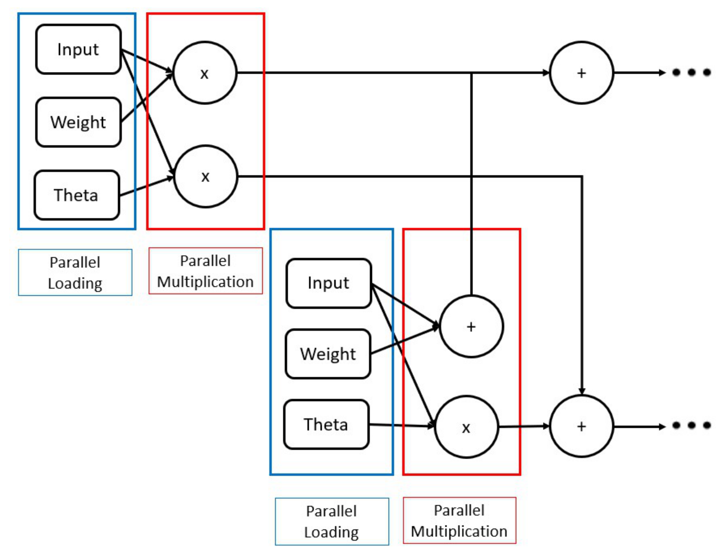
The benchmark dataset used from open-access traffic flow database of Caltrans Performance Measurement System (PeMS), U.S.A [56]. It consists of 51,406 samples that were divided into 60% training, 20% validation, and 20% testing. The PEMS data were collected every five minutes daily from 4 April to 27 November 2016 by a detector located on Route 22, Garden Grove. The model used six features: the day, the time in hours and minutes, the total miles that are driven by the vehicles, the total time spent by the vehicles, the speed detected by the detector, and the number of trucks for prediction.

6.2. Implementation

The training phase was implemented using python. In addition, the validation dataset was used to optimize all hyperparameters to obtain the smallest MAE. The best hyperparameters obtained β = 0.99, s = 0.2, and η = 0.00001 . They were chosen to provide the highest accuracy. The model was trained iteratively for seven epochs. Each epoch had two phases, which were training and testing. After reaching the seventh epoch, the Mean Absolute Error (MAE) was 0.001 and no more training was conducted for the model. The weights θ , w, and α were extracted to be used for hardware implementation. For efficient hardware implementation; the paper presents three different storage elements (BRAM, DDR, and distributed memory) to store and retrieve the weights. Each IP was implemented differently to support its corresponding memory. Additionally, the ONN models were implemented twice using 24 bit fixed and 32 bit floating points. Each IP is composed of three main matrix multiplications and additions. The multiplication in the first layer is between the input vector ( X ) feature and the weight vector θ 1 followed by an addition of one bias. The output is then multiplied by its weight α 1 . In the second layer, there exists two phases. The first phase is a matrix multiplication between X and w followed by the vector bias addition. The resultant output is a six unit vector fed to the second phase for multiplication by θ 2 and then one bias addition. The resultant output is then multiplied by its weight α 2 . The final prediction is the summation of the two layer outputs. Each IP implemented used a set of pragmas to optimize the code. These pragmas are listed below:
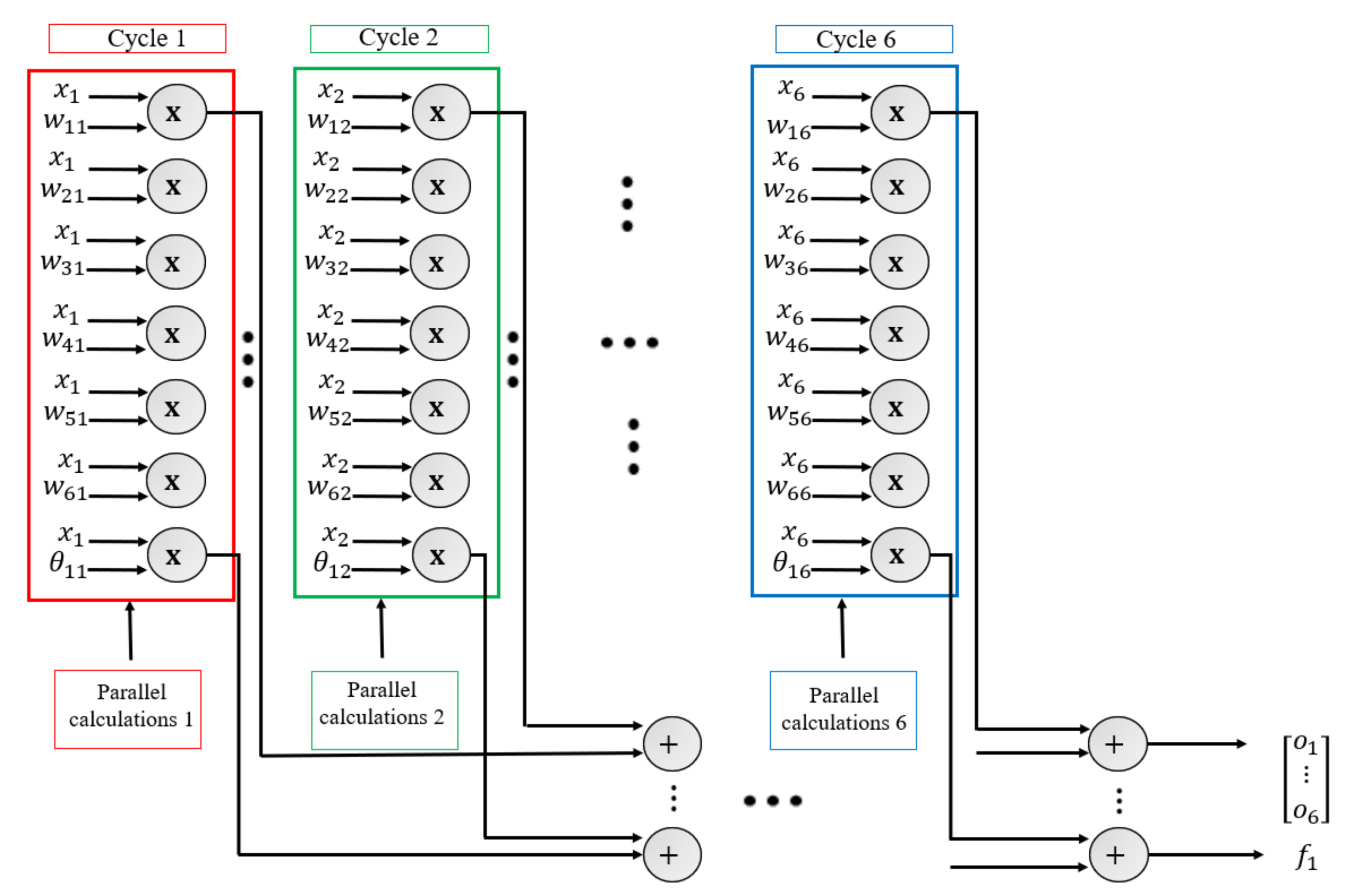
  • Pipelining: Pipelining pragma is used in high-level synthesis optimization techniques to improve the throughput of the system. This was conducted by allowing concurrent operations to take place inside the algorithm.
  • Allocation: This pragma is responsible for defining the limited number of resources inside a kernel. Consequently, it restricts the number of RTL examples and hardware resources such as (DSPs and BRAM) used for implementing particular loops, functions, operations, or cores.
  • Partitioning: Partitioning pragma is for arrays. It breaks up the large array into smaller arrays or individual elements (buffers). As a result, the accelerator can access the data, simultaneously resulting in high throughput but consumes high area resources.

6.2.1. Accelerator Design for the Distributed Memory Architecture

In this model, all weights are stored inside the IP core in distributed memory. Partitioning and allocation pragmas are added for design optimization. Partitioning weights are optimized in terms of latency. All weights were stored in registers to allow for multiple readings for computation at the same time. Consequently, the multiplications of w of layer 2 and θ of layer 1 are calculated simultaneously. By adding the allocation pragmas for addition and multiplications, the number of DSPs were reduced and reused for multiple calculations. As shown in Figure 3, the first block is executed; then, the next block makes use of the multipliers of the previous block. On the other hand, each time the weights need to be updated, the FPGA needs to be reprogrammed again. This includes updating the HLS code and regenerating the bitstream for the whole system in Vivado. It is considered an inefficient method for online neural network because weights need to be updated continuously.

6.2.2. Accelerator Design for the BRAM Architecture

The IP algorithm is implemented for storing weights inside a true dual port BRAM. The IP has five BRAM interfaces for the features, w, θ , b, and the result. For a fixed point, two pragmas are added (allocation and pipeline) for better resource allocation and latency. On the other hand, all of the other pragmas were tested and the pipeline pragma had the only effect inside the floating point architecture. A parallel performance occurs in loading weights and a feature and then multiplying for w in layer 2 and θ 1 for layer 1, as shown in Figure 4. Additionally, the implemented algorithm for the matrix multiplication between w and x was optimized such that the IP iterates through the elements of the input vector only once. Therefore, before moving to the next element in the input vector, each feature should finish its multiplications with all neurons weights. Each of theses multiplication results are stored in a vector. The size of this vector is equal to the number of neurons of this layer. Each element in the vector acts as an accumulator because its value is added to the multiplication of the next feature. In that way, the number of readings are reduced for the input reducing latency. Finally, the last matrix multiplication is executed between θ 2 and the output of (x and w 1 ).

6.2.3. Accelerator Design for the DDR Architecture

The IP architecture for DDR is very similar to the BRAM design in Figure 4. However, there is an extra logic added to support the AXI4 stream interface for w, θ 1 , θ 2 , and X. Those stream interfaces can only send integer numbers so there is a need to convert those integer numbers to either be floating or fixed inside the IP before starting the matrix multiplication. The output result is sent via the axi-lite interface. Pipeline, allocation, and partitioning pragmas are added for fixed point IP. On the contrary, only the pipeline pragma is added in the floating point IP because it is the only pragma that has an effect on the IP.

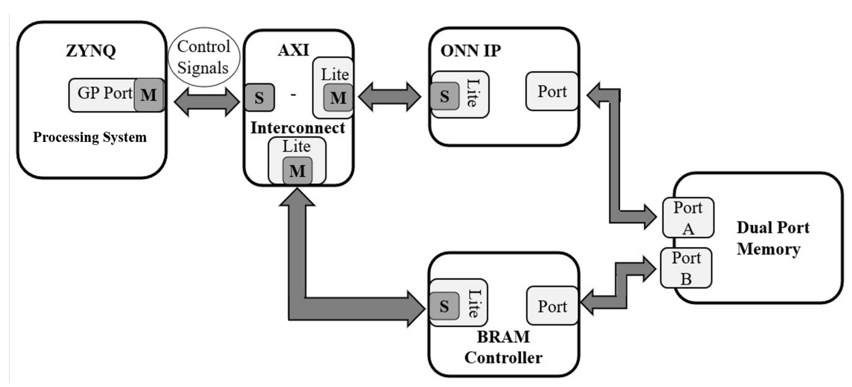
6.2.4. Whole System for the BRAM Design

This design is used when the size of the weights needed to be stored in the zedboard zynq-700 is less than or equal to 560 Kbits. This is the maximum size of the Block RAM (BRAM) inside the board. The size of the floating point weights is 2688 bits, while fixed point weights is 2016 bits, allowing the BRAM to store them. The BRAM system architecture consists of the Zynq processing system (ARM Processor), the ONN IP, AXI-Interconnect, five BRAM controllers, and five true dual port memories for accessing and storing (X, w, θ , b, and F). For simplicity, only one BRAM controller and one true dual port BRAM are shown in Figure 5. The Zynq processing system (ARM Processor) is connected to the ONN IP and BRAM controller using AXI-interconnect through the AXI3-(GP) General purpose Port. The AXI-interconnect converts the AXI3 to AXI4 lite interfaces for both the ONN IP and BRAM controller.
First, the Zynq processing system (ARM processor) sends the control signals for the ONN IP and BRAM controller. These control signals are responsible to initialize the IPs to check that they are free from errors and configured correctly. After initialization, the Zynq processing system sends the weights and features to be stored inside the BRAM. This is performed with the help of the BRAM controller, which has two ports, one connected to the Zynq processing system while the other connected to the AXI4 (memory mapped) slave interface. A true dual port memory is used so that the Zynq processing system and the IP access the memory simultaneously for faster prediction. Afterwards, the IP retrieves the weights and features for computation. Finally, the predicted output is stored back inside the BRAM and the results are shown on the Xilinx SDK tool.

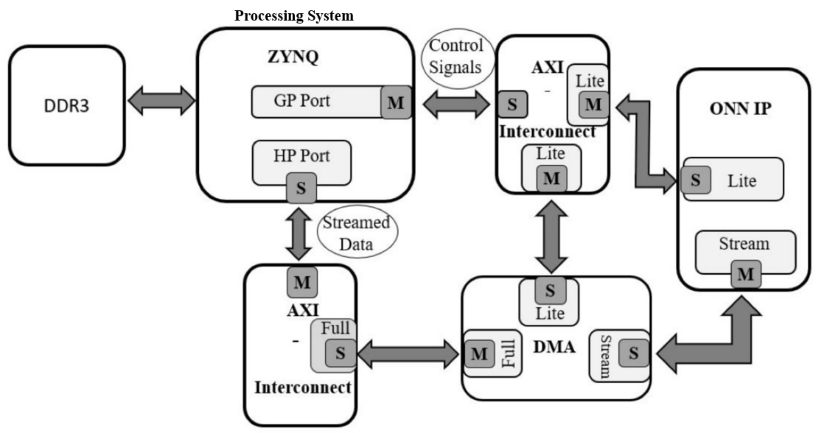
6.2.5. Whole System for DDR Design

This design is used when the weights are large in size and cannot be stored inside the BRAM. Although the weights used for traffic flow prediction were small in size, the DDR architecture was implemented to be analyzed and compared with the BRAM architecture. This system is composed of the Zynq processing system, Direct Memory Access (DMA), DDR3, an ONN IP accelerator, and AXI-Interconnect, as shown in Figure 6, similar to the BRAM design in which the the GP port using the AXI-Interconnect is used to send the control signals to both the ONN IP accelerator and the DMA for initialization.
In the beginning, the weights are stored inside the DDR3, which is inside the zedboard. The Zynq processing system has a high-performance port (HP), which is connected to the DMA AXI-Full port using AXI-Interconnect. It is responsible for streaming the data stored inside the DDR. Then, the weights are received at the IP accelerator by the master stream port, which is connected to the DMA. Finally, the IP executes the algorithm and sends the results back to the Zynq processing system using the AXI-Lite interface through the GP port.

6.2.6. Whole System for the Distributed Memory Design

The system for the distributed memory architecture is very similar to the BRAM system. However, it is a simpler design as it is composed of two BRAMs and two BRAM controllers for (X and F). As in Figure 5, the system is composed of the Zynq processing system to send features through the BRAM controller in a true dual port memory. Then, after the IP executes the algorithm, the output is stored back in another BRAM and the ARM processor is able to retrieve it.

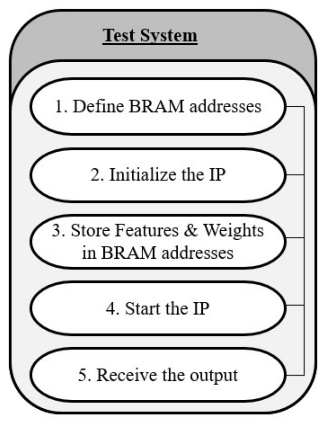
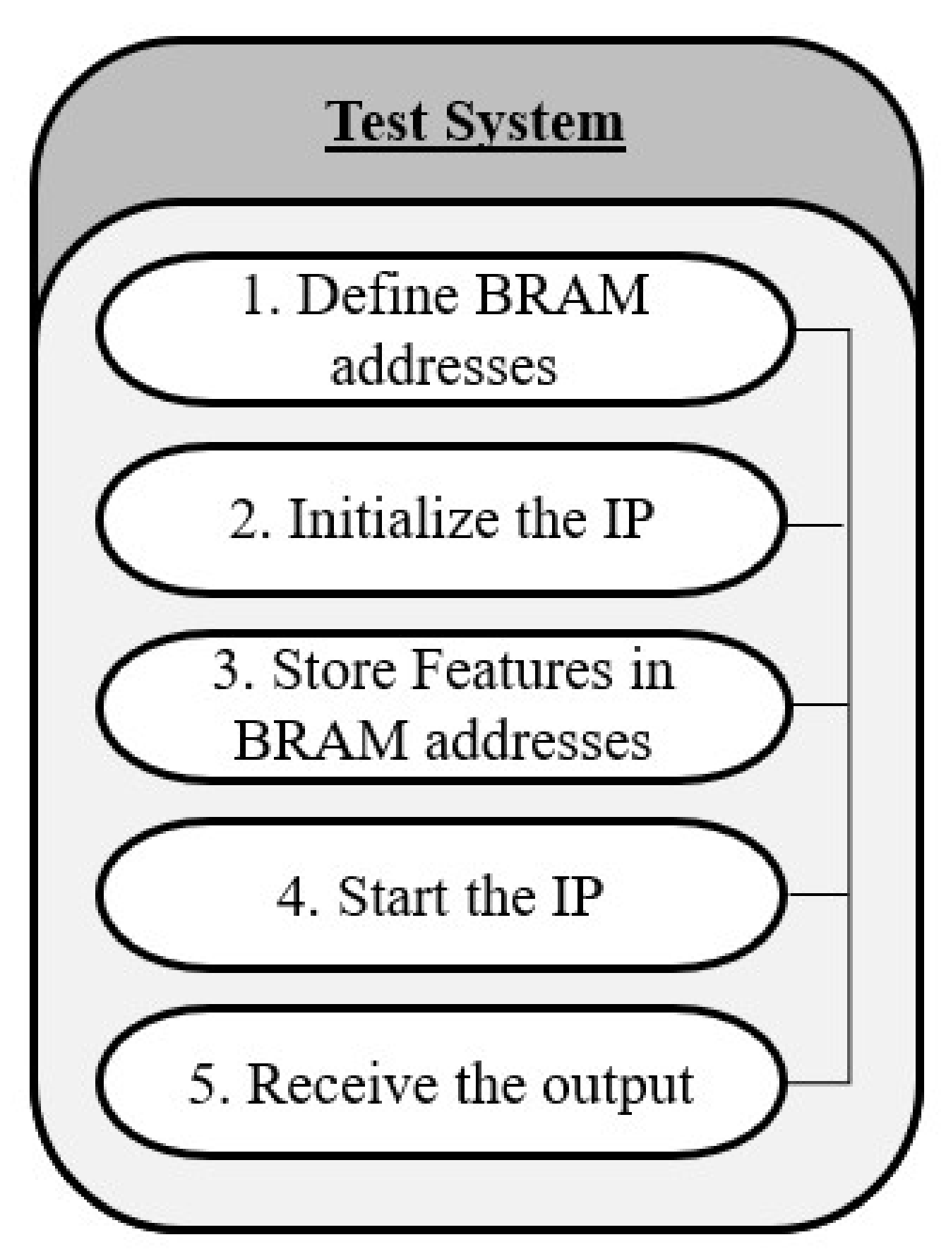
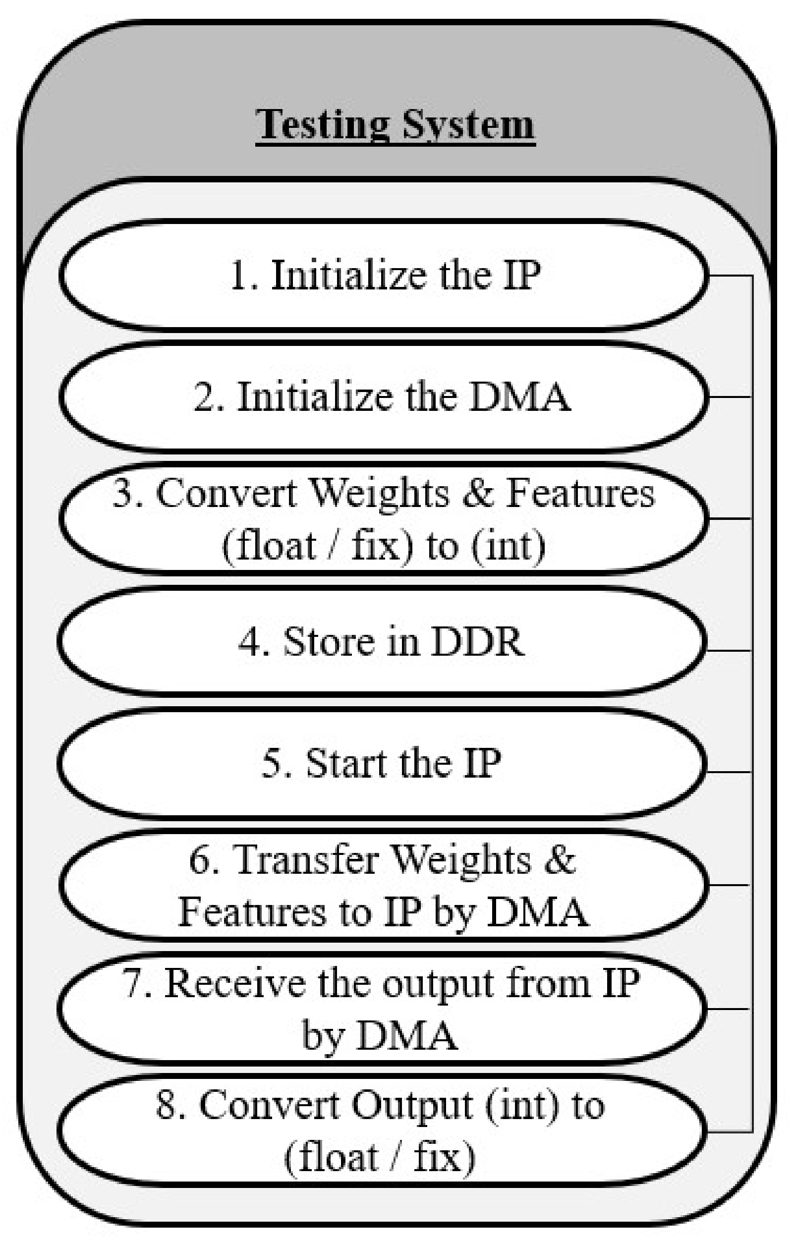
6.2.7. SDK Testing Environment

1. BRAM and Distributed Memory: Figure 7 shows how the system is tested on an FPGA using SDK tool for the BRAM system, while Figure 8 shows that for the distributed memory system. The two tests are very similar. For BRAM systems, the C++ code starts with defining the five BRAM addresses, while for distributed memory, only two BRAM addresses are defined. Second, the IPs are configured to be able to work. After that, inside the BRAM architecture, the weights and features are stored inside their corresponding BRAMs. On the contrary, only the features are stored inside the BRAM for distributed memory architecture. Then, the IPs access the BRAMs for calculations. When the predicted result is calculated, the IPs store it inside its BRAM. Finally, the processor retrieves the predicted output and shows the value in the console of Xilinx SDK.
2. DDR Figure 9 shows how the the system is tested on FPGA using Xillinx SDK. The IP and the four DMAs are configured and initialized. Then, all of the features and weights are converted to int to be stored in the DDR3. Furthermore, the IP starts; waiting for weights and features from the DMA. Then, the DMA sends the inputs, w, θ , and b to the IP for computation. When the IP finishes calculations, the result from the AXI-lite interface is then converted from int to either fixed/floating depending on the IP used.

7. Results and Discussion

The MLP consists of four layers: the input layer, two hidden layers, and the output layer. The input layer has six neurons, where each neuron connects directly to the six features. The 2 hidden layers have 100 neurons each, and the output layer has 1 neuron to calculate the traffic flow. A Relu function is used for all three layers except the output layer with no activation function. The model is optimized using the Adam technique. For the training phase, the MLP is trained for 50 epochs. This model was trained with varying batch size (1, 5, 10, and 15) to investigate its effect on MLP. From Table 1, it is clear that HBP provided the best result with MAE 0.001. Additionally, it should be noted that the batch size truly affects the error on MLP. The best two batch sizes are 1 and 15 with MAE 0.077 and 0.074, respectively.

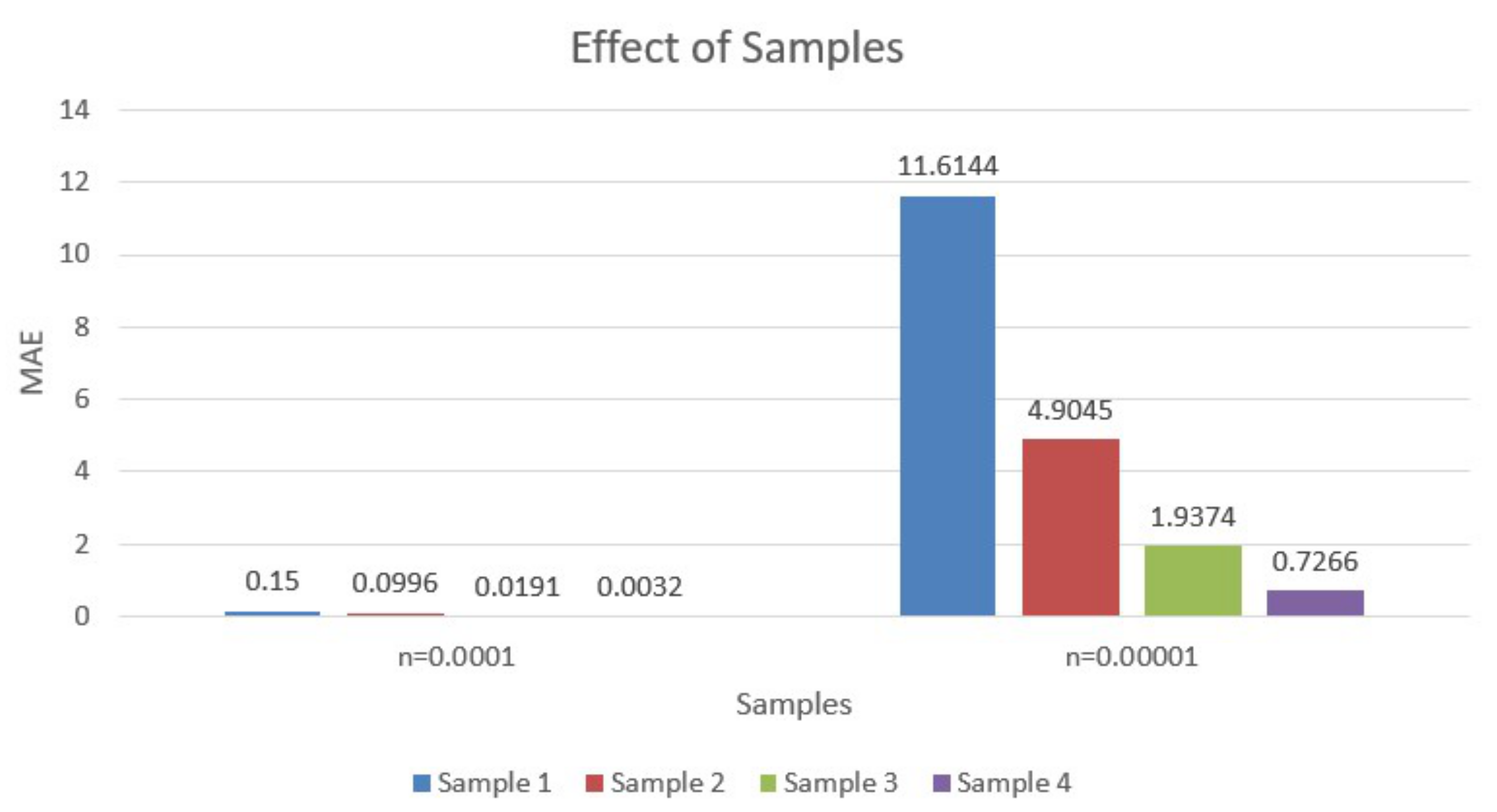
7.1. Performance Evaluation for Each Sample Set

The effect of varying data-set sizes is evaluated for the ONN model. The training data set is divided into four sample sets; each is 20% of the training set. The samples were used by the models for training with a batch size equal to 1 and for updating the weights and then testing the model on the testing set, which was 20% of the dataset. Therefore, whenever a new sample set is available, the set is taken to the model to train and update the weights and then to test it on the test set. This experiment is repeated five times, and the average values are taken. The following Figure 10 shows how ONN using the HBP model performs during the process of sampling. It is clear that the learning rate highly affects the performance of the model and that the learning rate with 0.0001 is better than that with 0.000001. Additionally, the figure shows that the model improves its performance when the whole dataset is passed to the model.

7.2. Hardware Timing Analysis

In this section, a timing analysis is conducted. It compares the execution time between the online hardware NN IP and the whole system configuration with the ARM processor as well as between the software execution time. As mentioned in Section 5, there are six different IP cores to support six system architectures. The execution time of the hardware ONN IPs is calculated by extracting the number of clock cycles required for traffic flow prediction multiplied by the clock of the PL. On the other hand, the processing time of the complete system is measured by counting the number of ARM processor’s clock cycles spent obtaining the prediction from SDK. The PL is clocked at 100 Mhz, while the ARM processor runs at 650 MHz. As shown in Table 2, all ONN IP latencies are smaller than the whole system latency.
The reason behind that is the communication overhead between the ARM processor and the IP core from AXI-interconnect and routing. Additionally, Table 2 shows that the latency for the distributed memory is the smallest. The weights are stored inside the IP as registers. They can be accessed multiple of times at the same time, allowing for parallel calculations. Unlike BRAM, which needs to be accessed once from the IP each clock cycle, the BRAM latencies produced from IP and system are less than the DDR latencies. The reasons are listed below:
  • IP model: The code that converts int to float for the DDR architecture consumes some time inside the IP block, unlike the BRAM architecture, which stores the weight inside it in float or fixed without converting them to the integer format. Hence, BRAM IP block is faster than DDR block.
  • System: Routing and placement inside any FPGA affects the timing of the system. The DDR is placed as an external memory on the PS side of the zedboard, while the BRAM is located inside the PL. This means that the BRAM is located closer to the IP than DDR. Therefore, the communication time between the IP and the BRAM is faster and that the latency is lower than DDR.
Additionally, it is shown that the latency of the fixed point format is faster than the floating point format. This is because the calculations for a fixed point is simpler and requires a smaller number of operations compared with floating point operations. Finally, the software execution time was extracted from python and was 100,000 ns, which is 200X slower than the hardware. Consequently, it is concluded that all of the hardware models proposed perform better than the software model.

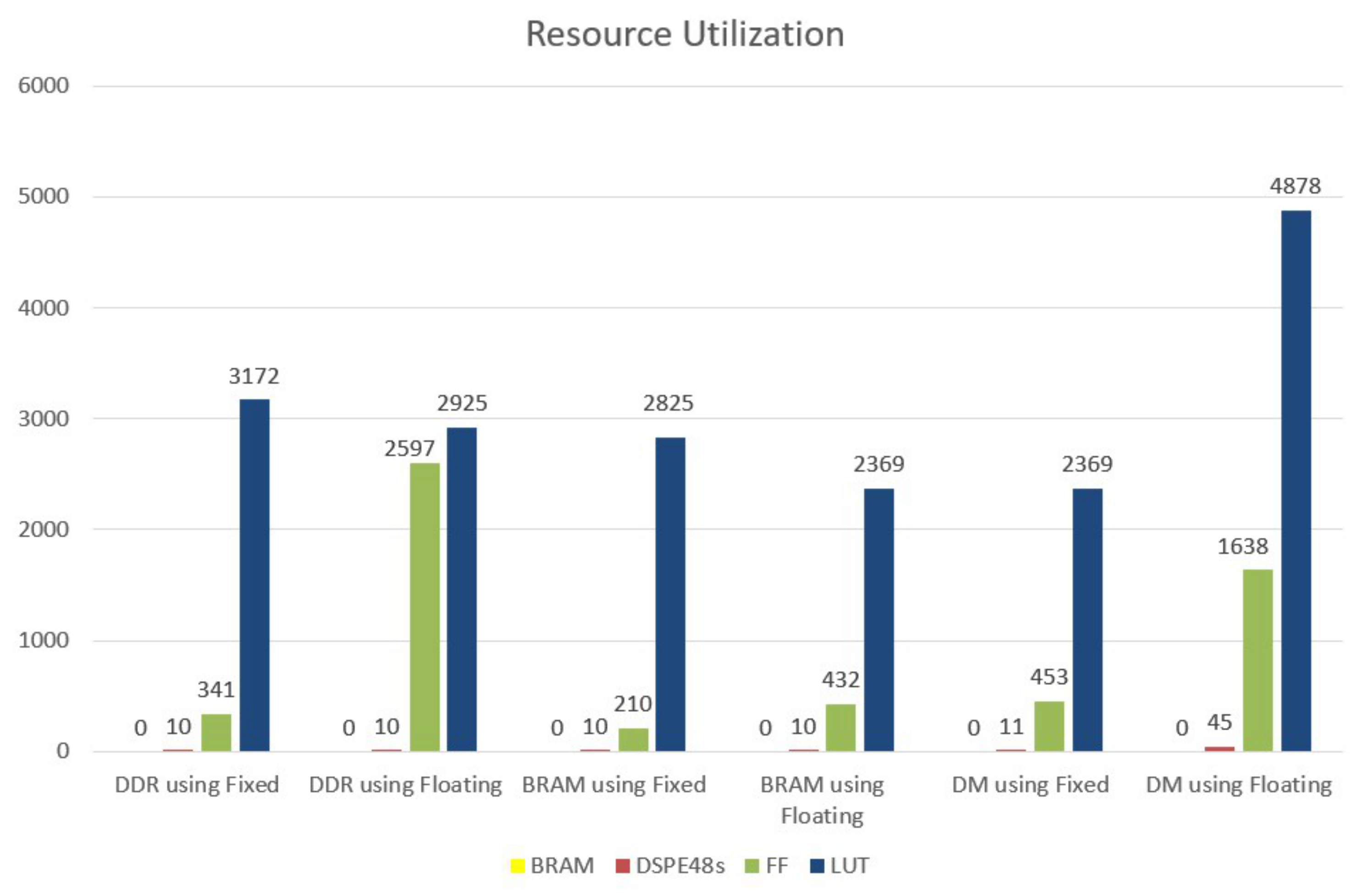
7.3. Hardware Resource Utilization Analysis

In this section, the six different IP ONN models are analyzed in terms of resource utilization. They have been synthesized and implemented on zedboard to obtain the utilization of the six different versions. Vivado 2017.4 is used to report them. Figure 11 conveys that the BRAM architecture with fixed points has the least number of flipflops. In addition, DDR using fixed and BRAM with fixed and floating points have only 10 DSPs, which represents a small number in comparison with the others.

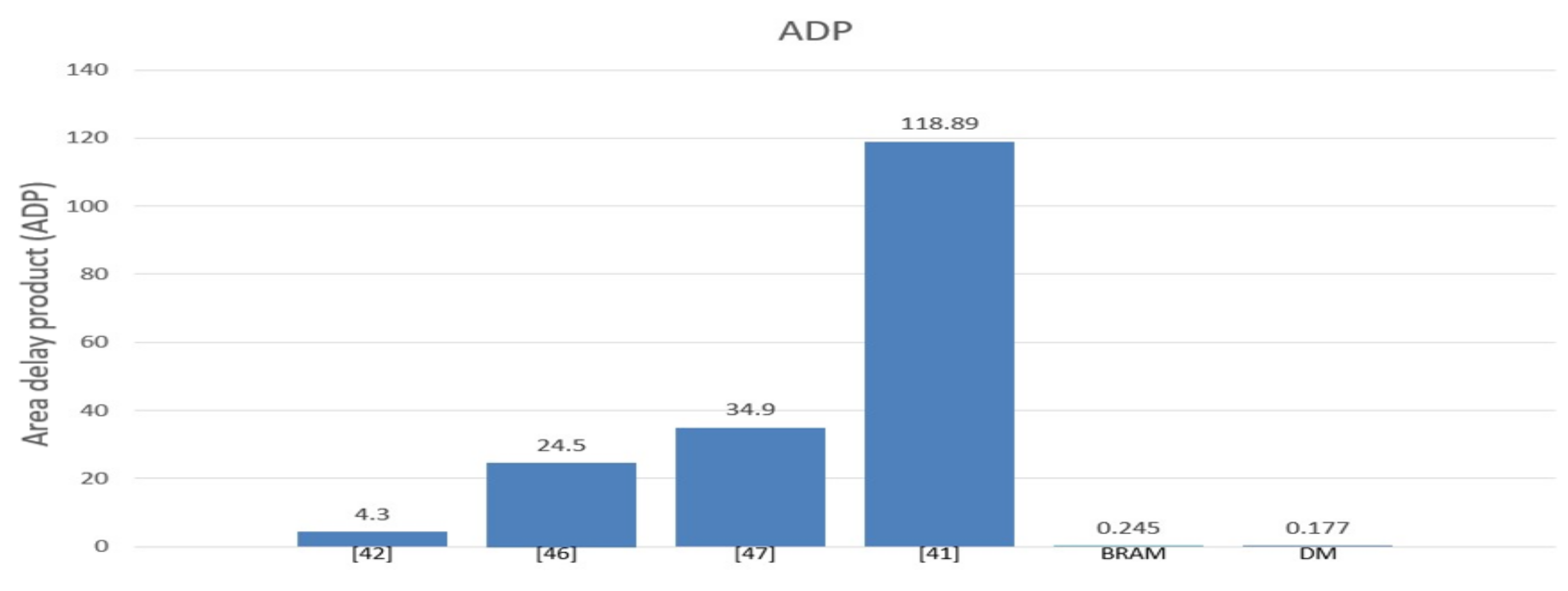
7.4. Area-Delay Product (ADP)

Area-Delay Product (ADP) is a metric used in this paper to evaluate the overall performance with respect to both utilization and execution time among all previous work. Since some models are good in terms of utilization but have high latency and vice versa, a metric is needed that can measure both utilization and latency together. It was very hard to find a suitable metric in papers that can be taken as a reference to measure both latency and utilization together. Therefore, this metric was designed to fulfil this aim. This proposed metric behaves similar to the concept of a power delay product metric but replaces the power with utilization. It is defined in Equation (22). There are some differences between the ADP and the power delay product. The first thing is that in case the model does not have a specific parameter in the equation, it is excluded. In addition, the number in the denominator reduces the value of the ADP to a small number for easier representation. The smaller the Area Delay product number, the better the design in terms of latency and utilization. The same formula was applied to previous work for consistency and compared with our design.
As shown in Figure 12, the ADP of the MLP with HBP using distributed memory has the smallest value followed by the ONN using BRAM. Therefore, it is clear that the hardware ONN outperforms all previous work by factors of 24X and 17X, respectively.
A D P = L U T * F F * B R A M * D S P * L a t e n c y 10 10

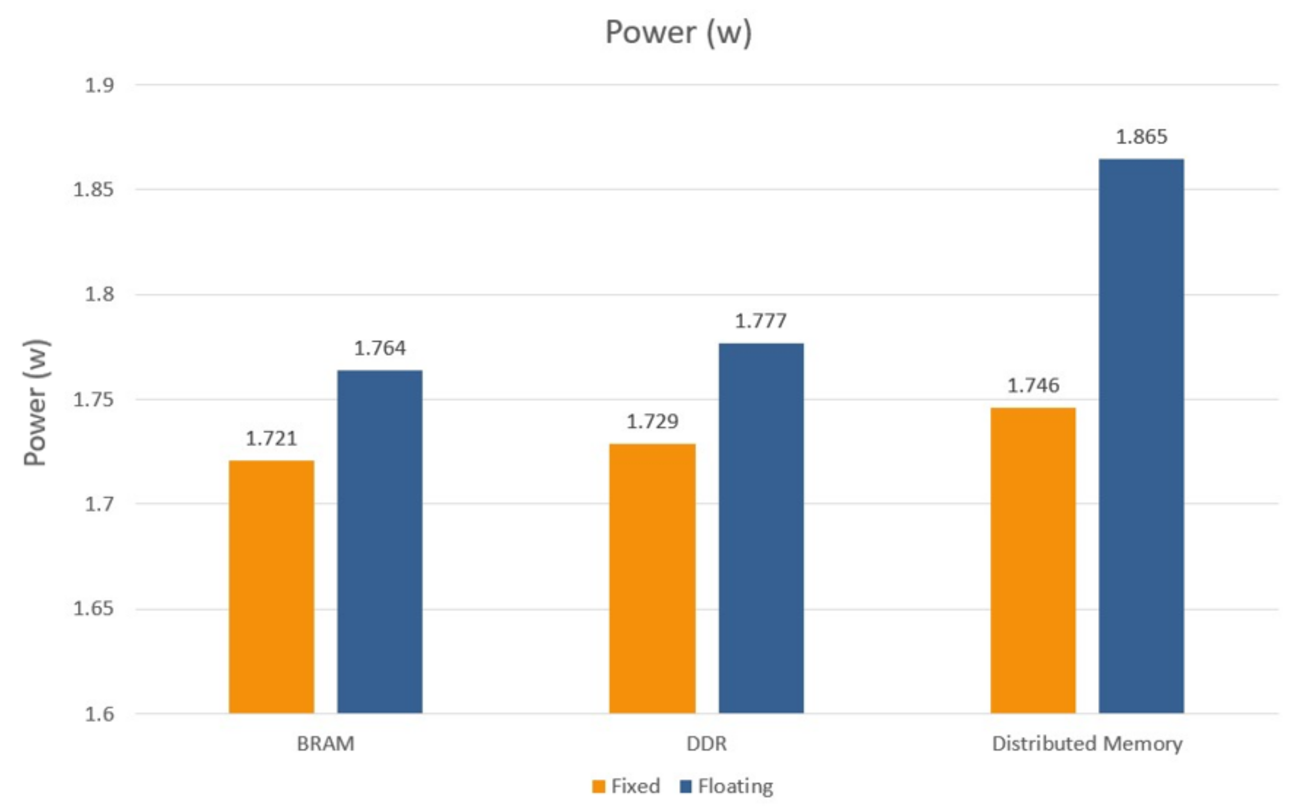
7.5. Power Consumption Analysis

The total on-chip power consumption that combines both static and dynamic power is shown in Figure 13. The static power is consumed in signals, logic, DSP, BRAM, and Ps7 and is affected by the clocked frequency. Since the ARM processor is clocked at a high frequency 650 MHz, it consumes the highest power in the system. The data was extracted from the power report produced from the Vivado tool. The diagram shows that the IP with a fixed point and BRAM architecture has the smallest power, equal to 1.721W. This result is expected since the BRAM architecture using a fixed point has the least resources.

7.6. Online Compatibility

Previous work implemented offline models and always assumed that the weights are completely fixed, i.e., does not change with time. As a result, designers store their weights in distributed memory (LUT) since it is the fastest memory type compared with BRAM and DDR. However, this paper aims to design an online neural network (ONN) known for learning the model from sequential data instances one at a time. This means that the weights are updated continuously. As a result, the parameters used for inference need to be stored in a memory that can be updated in real time. The data inside the DDR and BRAM memory can be updated without modifying the HLS code using the Xilinx SDK tool. Therefore, they are suitable for online machine learning algorithms. However, it should be noted that fixed point models have lower latency, utilization, and power than floating point models. Additionally, there is no degradation in the accuracy using either fixed or floating point. This is because the output from the model is rounded up to a whole number. The ONN model does not need to produce an accurate decimal number. In consequence, fixed point is preferable to floating point in traffic flow prediction. The ONN using distributed memory (LUT) was only implemented for comparison with existing works.

7.7. Comparison with Existing Works

Based on the state-of-the-art, the MLP using HBP has never been implemented on hardware before. Consequently, it was impossible to compare our design with an identical one (same number of layers, topology, and application). As explained before, MLP using HBP is a modified version of MLP so it was compared with other MLP topologies. The previously proposed architectures found in the literature are the closest possible architectures to our design.
Table 3 shows a comparison of the hardware ONN model using HBP with some previous hardware MLP models. As shown in Table 3, the online neural network typologies for both distributed memory and BRAM storage have the smallest latencies, 150 ns and 420 ns, respectively. Finally, the LUT in a distributed memory system is reduced by 20.6% and the DSPs in the BRAM system is reduced by 16%.

8. Conclusions

This research proposes a highly accurate traffic flow prediction system using an online neural network. The model with a (6-1)/(6-1) topology has a higher accuracy in comparison with the normal MLP with varying batch size (1, 5, 10, and 15) and MLR. The HBP model provides the best result, with MAE 0.001. In addition, this paper implements different hardware architectures for the proposed system to achieve the most suitable design in terms of latency, utilization, and power. The BRAM architecture and distributed memory architecture provide the most adequate solution for the abovementioned aspects. The BRAM requires only 420 nanoseconds for prediction while distributed memory requires 150 nanoseconds. However, an important metric that should be taken into account is the online compatibility. It allows hardware designers to choose the most suitable system for online learning. DDR and BRAM are compatible, while the distributed memory is not suitable for online learning. This is because the weights in the distributed memory are hard coded (fixed) inside the HLS code. However, in online learning, the weights continuously update. The DDR architecture is used when the weights of the model are larger than 4.9 Mb, while the BRAM architecture is very suitable for applications in which the weights size is smaller than 4.9 Mb. This value is obtained from the zedboard datasheet. It is preferable for online machine learning designers to use the BRAM architecture for ONN because it has less latency than the DDR architecture given that latency is the most important parameter in online applications. Consequently, for larger designs, it is recommended for designers to use larger FPGA boards that have larger BRAM capacity. Moreover, it is recommended to use fixed point instead of floating point because fixed point models have lower latency, utilization, and power than floating point models. The fixed point models did not have any degradation in accuracy because the number of cars are rounded up and an exact decimal number is not needed. Additionally, the ADP of the ONN using BRAM is 17X better than the newest MLP model. Moreover, the execution time of the hardware implementation using BRAM on the zedboard zynq-700 improved by a factor of 200X compared with the software implementation on a dual-core Intel i7-7500U CPU at 2.9 GHz. Finally, these results recommend that the BRAM architecture using fixed point is the most suitable one for online machine learning algorithms.

9. Future Work

In this study, the training phase was performed using python software and the weights were extracted to be used in the hardware ONN model. This can be altered by implementing the training part inside the ARM processor of the ZYNQ board. The weights are directly transferred from the PS to the PL without the intermediate part of python. Additionally, the training phase can be implemented using both fixed point and floating point. In addition, the inference as well as the training parts of the ONN model can be implemented using any HDL language. Hence, the HLS tool does not synthesize the C/C++ code to HDL. This implementation can be compared with the HLS ONN model in terms of latency, utilization, and power. Finally, the HBP algorithm, which is used for updating ( α ) the weights assigned for each expert, can be altered with new algorithms and can compare these new algorithms with HBP.

Author Contributions

Conceptualization, software, validation, investigation, and writing—original draft preparation, Y.A.H.; writing—review and editing, Y.A.H., M.M. and M.A.A.E.G.; supervision, M.M. and M.A.A.E.G. All authors have read and agreed to the published version of the manuscript.

Funding

This research received no external funding.

Conflicts of Interest

The authors declare no conflict of interest.

Abbreviations

The following abbreviations are used in this manuscript:
ADAM(Adaptive Momentum)
ADP(Area-Delay Product)
AI(Artificial Intelligence)
ANN(Artificial Neural Network)
AXI(Advance eXtensible Interface)
BRAM(Block RAM)
CalTrans(California Transportation Agencies)
CNN(Convolution Neural Network)
DBN(Deep Belief Network)
DCRNN(Diffusion Convolutional Recurrent Neural Network)
DSP(Digital Signal Processing)
FF(Flip Flop)
FPGA(Field-Programmable Gate Array)
GBRT(Gradient Boosting Regression Trees)
GDGradient Descent
HDL(Hardware Design Language)
HLS(High Level Synthesis)
ITS(Intelligent Transport System)
LR(Linear Regression)
LUT(Look-Up Table)
LSTM(Long Short Term Memory)
MAE(Mean Absolute Error)
ML(Machine Learning)
MLR(Multiple Linear Regression)
MLP(Multi-Layer Perceptron)
MTL(Multi-Task regression Layer)
NN(Neural Networks)
PeMs(Performance Measurement System)
PL(Programmable Logic)
PS(Processing System)
Relu(Rectifier Linear Unit)
RF(Random Forest)
RMSE(Root Mean Square Error)
RMSprop(Root Mean Square Propagation)
SAE(Stacked Auto Encoder)
SDK(Software Development Kit)
SGD(Stochastic Gradient Descent)
SVR(Support Vector)
XGB(Extreme Gradient Boosting Regression Trees)

References

  1. Petrosino, A.; Maddalena, L. Neural networks in video surveillance: A perspective view. In Handbook on Soft Computing for Video Surveillance; Chapman and Hall/CRC: Boca Raton, FL, USA, 2012. [Google Scholar]
  2. Nassif, A.B.; Shahin, I.; Attili, I.; Azzeh, M.; Shaalan, K. Speech Recognition Using Deep Neural Networks: A Systematic Review. IEEE Access 2019, 7, 19143–19165. [Google Scholar] [CrossRef]
  3. Havaei, M.; Davy, A.; Warde-Farley, D.; Biard, A.; Courville, A.; Bengio, Y.; Pal, C.; Jodoin, P.; Larochelle, H. Brain Tumor Segmentation with Deep Neural Networks. Med. Image Anal. 2017, 35, 18–31. [Google Scholar] [CrossRef] [PubMed] [Green Version]
  4. Dong, Y.; Hu, Z.; Uchimura, K.; Murayama, N. Driver Inattention Monitoring System for Intelligent Vehicles: A Review. IEEE Trans. Intell. Transp. Syst. 2011, 12, 596–614. [Google Scholar] [CrossRef]
  5. Goswami, S.; Chakraborty, S.; Ghosh, S.; Chakrabarti, A.; Chakraborty, B. A review on application of data mining techniques to combat natural disasters. Ain Shams Eng. J. 2016, 9, 365–378. [Google Scholar] [CrossRef] [Green Version]
  6. Ngai, E.W.; Xiu, L.; Chau, D.C. Application of data mining techniques in customer relationship management: A literature review and classification. Expert Syst. Appl. 2009, 36, 2592–2602. [Google Scholar] [CrossRef]
  7. Yang, Y.; Wu, Y.; Zhan, D.; Liu, Z.; Jiang, Y. Complex Object Classification: A Multi-Modal Multi- Instance Multi-Label Deep Network with Optimal Transport. In Proceedings of the 24th ACM SIGKDD International Conference on Knowledge Discovery & Data Mining, London, UK, 19–23 August 2018; pp. 2594–2603. [Google Scholar]
  8. Ghazwan, J. Application of neural network to optimize oil field production. Asian Trans. Eng. 2012, 2, 10–23. [Google Scholar]
  9. Srivastava, R.K.; Greff, K.; Schmidhuber, J. Training very deep networks. arXiv 2015, arXiv:1507.06228. [Google Scholar]
  10. Tan, H.H.; Lim, K.H. Vanishing Gradient Mitigation with Deep Learning Neural Network Optimization. In Proceedings of the 2019 7th International Conference on Smart Computing & Communications (ICSCC), Sarawak, Malaysia, 28–30 June 2019; pp. 1–4. [Google Scholar]
  11. Ioffe, S.; Szegedy, C. Batch normalization: Accelerating deep network training by reducing internal covariate shift. In Proceedings of the 32nd International Conference on International Conference on Machine Learning (ICML’15), Lille, France, 6–11 July 2015; Volume 37, pp. 448–456. [Google Scholar]
  12. Choromanska, A.; Henaff, M.; Mathieu, M.; Arous, G.; LeCun, Y. The loss surfaces of multilayer networks. J. Mach. Learn. Res. 2015, 38, 192–204. [Google Scholar]
  13. Zhang, C.; Liu, L.; Lei, D.; Yuan, Q.; Zhuang, H.; Hanratty, T.; Han, J. TrioVecEvent: Embedding-Based Online Local Event Detection in Geo-Tagged Tweet Streams. In Proceedings of the 23rd ACM SIGKDD International Conference, Halifax, NS, Canada, 13–17 August 2017; pp. 595–604. [Google Scholar]
  14. Sahoo, D.; Pham, Q.; Lu, J.; Hoi, S.C.H. Online Deep Learning: Learning Deep Neural Networks on the Fly. arXiv 2017, arXiv:1711.03705. [Google Scholar]
  15. Yang, Y.; Zhou, D.; Zhan, D.; Xiong, H.; Jiang, Y. Adaptive Deep Models for Incremental Learning: Considering Capacity Scalability and Sustainability. In Proceedings of the 25th ACM SIGKDD International Conference on Knowledge Discovery & Data Mining (KDD’19), Anchorage, AK, USA, 4–8 August 2019; Association for Computing Machinery: New York, NY, USA, 2019; pp. 74–82. [Google Scholar]
  16. Pratama, M.; Za’in, C.; Ashfahani, A.; Soon, O.; Ding, W. Automatic Construction of Multi-layer Perceptron Network from Streaming Examples. In Proceedings of the 28th ACM International Conference on Information and Knowledge Management (CIKM 2019), Beijing, China, 3–7 November 2019. [Google Scholar]
  17. Zinkevich, M. Online convex programming and generalized infinitesimal gradient ascent. In Proceedings of the Twentieth International Conference on Machine Learning (ICML’03), Washington, DC, USA, 21–24 August 2003; pp. 928–935. [Google Scholar]
  18. Hanafy, Y.A.; Gazya, M.; Mashaly, M.; Abd El Ghany, M.A. A Comparison between Adaptive Neural Networks Algorithms for Estimating Vehicle Travel Time. In Proceedings of the 15th International Conference on Computer Engineering and Systems (ICCES 2020), Cairo, Egypt, 15–16 December 2020. [Google Scholar]
  19. Kumar, K.; Parida, M.; Katiyar, V.K. Short term traffic flow prediction in heterogeneous condition using artificial neural network. Transport 2013, 30, 1–9. [Google Scholar] [CrossRef]
  20. Ma, X.; Dai, Z.; He, Z.; Ma, J.; Wang, Y.; Wang, Y. Learning Traffic as Images: A Deep Convolutional Neural Network for Large-Scale Transportation Network Speed Prediction. Sensors 2017, 17, 818. [Google Scholar] [CrossRef] [Green Version]
  21. Jin, Y.L.; Xu, W.R.; Wang, P.; Yan, J.Q. SAE network: A deep learning method for traffic flow prediction. In Proceedings of the 5th International Conference on Information, Cybernetics, and Computational Social Systems (ICCSS), Hangzhou, China, 16–19 August 2018; pp. 241–246. [Google Scholar]
  22. Zhao, X.; Gu, Y.; Chen, L.; Shao, Z. Urban Short-Term Traffic Flow Prediction Based on Stacked Autoencoder. In 19th COTA International Conference of Transportation Professionals; American Society of Civil Engineers: Nanjing, China, 2019; pp. 5178–5188. [Google Scholar]
  23. Zhao, P.; Cai, D.; Zhang, S.; Chen, F.; Zhang, Z.; Wang, C.; Li, J. Layerwise Recurrent Autoencoder for General Real-world Traffic Flow Forecasting. In Proceedings of the International Conference on Learning Representations (ICLR), New Orleans, LA, USA, 6–9 May 2019. [Google Scholar]
  24. Voulodimos, A.; Doulamis, N.; Doulamis, A.; Protopapadakis, E. Deep Learning for Computer Vision: A Brief Review. Comput. Intell. Neurosci. 2018. [Google Scholar] [CrossRef]
  25. Alajali, W.; Zhou, W.; Wen, S. Traffic Flow Prediction for Road Intersection Safety. In Proceedings of the 2018 IEEE SmartWorld, Ubiquitous Intelligence & Computing, Advanced & Trusted Computing, Scalable Computing & Communications, Cloud & Big Data Computing, Internet of People and Smart City Innovation (SmartWorld/SCALCOM/UIC/ATC/CBDCom/IOP/SCI), Guangzhou, China, 8–12 October 2018; pp. 812–820. [Google Scholar]
  26. Sharma, B.; Agnihotri, S.; Tiwari, P.; Yadav, P.; Nezhurina, M. Ann based short-term traffic flow forecasting in undivided two lane highway. J. Big Data 2018, 5, 1–16. [Google Scholar] [CrossRef]
  27. Romeiko, X.X.; Guo, Z.; Pang, Y.; Lee, E.K.; Zhang, X. Comparing Machine Learning Approaches for Predicting Spatially Explicit Life Cycle Global Warming and Eutrophication Impacts from Corn Production. Sustainability 2020, 12, 1481. [Google Scholar] [CrossRef] [Green Version]
  28. Pun, L.; Zhao, P.; Liu, X. A multiple regression approach for traffic flow estimation. IEEE Access 2019, 7, 35998–36009. [Google Scholar] [CrossRef]
  29. Huang, W.; Song, G.; Hong, H.; Xie, K. Deep architecture for traffic flow prediction: Deep belief networks with multitask learning. IEEE Trans. Intell. Transp. Syst. 2014, 15, 2191–2201. [Google Scholar] [CrossRef]
  30. Zhang, J.; Zheng, Y.; Qi, D. Deep spatio-temporal residual networks for citywide crowd flows prediction. In Proceedings of the Thirty-First AAAI Conference on Artificial Intelligence (AAAI’17), San Francisco, CA, USA, 4–9 February 2017; pp. 1655–1661. [Google Scholar]
  31. Yu, R.; Li, Y.; Shahabi, C.; Demiryurek, U.; Liu, Y. Deep Learning: A Generic Approach for Extreme Condition Traffic Forecasting. In Proceedings of the SIAM International Conference on Data Mining, Houston, TX, USA, 30 July 2017; pp. 777–785. [Google Scholar]
  32. Li, Y.; Yu, R.; Shahabi, C.; Liu, Y. Diffusion convolutional recurrent neural network: Data-driven traffic forecasting. arXiv 2017, arXiv:1707.01926. [Google Scholar]
  33. Zhou, J.; Chang, H.; Cheng, X.; Zhao, X. A Multiscale and High-Precision LSTM-GASVR Short-Term Traffic Flow Prediction Model. Complexity 2020. [Google Scholar] [CrossRef]
  34. Rusu, A.A.; Rabinowitz, N.C.; Desjardins, G.; Soyer, H.; Kirkpatrick, J.; Kavukcuoglu, K.; Pascanu, R.; Hadsell, R. Progressive Neural Networks. arXiv 2016, arXiv:1606.04671. [Google Scholar]
  35. Jin, R.; Hoi, S.; Yang, T. Online multiple kernel learning: Algorithms and mistake bounds. In International Conference on Algorithmic Learning Theory; Springer: Berlin/Heidelberg, Germany, 2010; Volume 6331, pp. 390–404. [Google Scholar]
  36. Sahoo, D.; Hoi, S.; Zhao, P. Cost Sensitive Online Multiple Kernel Classification. In Proceedings of the Eighth Asian Conference on Machine Learning, Hamilton, New Zealand, 16–18 November 2016; Volume 63, pp. 65–80. [Google Scholar]
  37. Lee, S.-W.; Lee, C.-Y.; Kwak, D.-H.; Kim, J.; Kim, J.; Zhang, B.-T. Dual-memory deep learning architectures for lifelong learning of everyday human behaviors. In Proceedings of the Twenty-Fifth International Joint Conference on Artificial Intelligence (IJCAI), New York, NY, USA, 9–15 July 2016; pp. 1669–1675. [Google Scholar]
  38. Yoon, J.; Yang, E.; Lee, J.; Hwang, S.J. Lifelong learning with dynamically expandable networks. arXiv 2017, arXiv:1708.01547. [Google Scholar]
  39. Misra, J.; Saha, I. Artifcial neural networks in hardware: A survey of two decades of progress. Neurocomputing 2010, 74, 239–255. [Google Scholar] [CrossRef]
  40. Subadra, M.; Lakshmi, K.P.; Sundar, J.; MathiVathani, K. Design and implementation of multilayer perceptron with on-chip learning in virtex-e. AASRI Procedia 2014, 6, 82–88. [Google Scholar]
  41. Gaikwad, N.B.; Tiwari, V.; Keskar, A.; Shivaprakash, N.C. Efficient fpga implementation of multilayer perceptron for real-time human activity classification. IEEE Access 2019, 7, 26696–26706. [Google Scholar] [CrossRef]
  42. Ortigosa, E.M.; Ortigosa, P.M.; Cañas, A.; Ros, E.; Agís, R.; Ortega, J. Fpga implementation of multi-layer perceptrons for speech recognition. In Field Programmable Logic and Application; Springer: Berlin/Heidelberg, Germany, 2003; pp. 1048–1052. [Google Scholar]
  43. Basterretxea, K.; Echanobe, J.; del Campo, I. A wearable human activity recognition system on a chip. In Proceedings of the 2014 Conference on Design and Architectures for Signal and Image Processing, Madrid, Spain, 8–10 October 2014; pp. 1–8. [Google Scholar]
  44. Chalhoub, N.; Muller, F.; Auguin, M. Fpga-based generic neural network architecture. In Proceedings of the 2006 International Symposium on Industrial Embedded Systems, Antibes Juan-Les-Pins, France, 18–20 October 2006; pp. 1–4. [Google Scholar]
  45. Alilat, F.; Yahiaoui, R. Mlp on fpga: Optimal coding of data and activation Function. In Proceedings of the 10th IEEE International Conference on Intelligent Data Acqui-sition and Advanced Computing Systems: Technology and Applications (IDAACS), Metz, France, 18–21 September 2019; Volume 1, pp. 525–529. [Google Scholar]
  46. Zhai, X.; Ali, A.A.S.; Amira, A.; Bensaali, F. MLP Neural Network Based Gas Classification System on Zynq SoC. IEEE Access 2016, 4, 8138–8146. [Google Scholar] [CrossRef]
  47. Pano-Azucena, A.; Tlelo-Cuautle, E.; Tan, S.; Ovilla-Martinez, B.; de la Fraga, L. Fpga-based implementation of a multilayer perceptron suitable for chaotic time series prediction. Technologies 2018, 6, 90. [Google Scholar] [CrossRef] [Green Version]
  48. Jia, T.; Guo, T.; Wang, X.; Zhao, D.; Wang, C.; Zhang, Z.; Lei, S.; Liu, W.; Liu, H.; Li, X. Mixed natural gas online recognition device based on a neural network algorithm implemented by an fpga. Sensors 2019, 19, 2090. [Google Scholar] [CrossRef] [Green Version]
  49. Singh, S.; Sanjeevi, S.; Suma, V.; Talashi, A. Fpga implementation of a trained neural network. IOSR J. Electron. Commun. Eng. IOSR JECE 2015, 10, 45–54. [Google Scholar]
  50. Zhang, L. Artificial neural network model-based design and fixed-point FPGA implementation of hénon map chaotic system for brain research. In Proceedings of the 2017 IEEE XXIV International Conference on Electronics, Electrical Engineering and Computing (INTERCON), Cusco, Peru, 15–18 August 2017; pp. 1–4. [Google Scholar]
  51. Bahoura, M. FPGA Implementation of Blue Whale Calls Classifier Using High-Level Programming Tool. Electronics 2016, 5, 8. [Google Scholar] [CrossRef] [Green Version]
  52. Bratsas, C.; Koupidis, K.; Salanova, J.-M.; Giannakopoulos, K.; Kaloudis, A.; Aifadopoulou, G. A Comparison of Machine Learning Methods for the Prediction of Traffic Speed in Urban Places. Sustainability 2020, 12, 142. [Google Scholar] [CrossRef] [Green Version]
  53. Kingma, D.P.; Ba, J. Adam: A method for stochastic optimization. arXiv 2014, arXiv:1412.6980. [Google Scholar]
  54. Hoi, S.C.H.; Sahoo, D.; Lu, J.; Zhao, P. Online Learning: A Comprehensive Survey. arXiv 2018, arXiv:1802.02871. [Google Scholar]
  55. Freund, Y.; Schapire, R.E. A decision-theoretic generalization of online learning and an application to boosting. J. Comput. Syst. Sci. 1997, 55, 119–139. [Google Scholar] [CrossRef] [Green Version]
  56. Caltrans, Performance Measurement System (PeMS). Available online: http://pems.dot.ca.gov/ (accessed on 17 May 2020).
Figure 1. A 2 layer MLP model.
Electronics 10 01875 g001
Figure 2. A 2 layer HBP model.
Electronics 10 01875 g002
Figure 3. IP design for distributed memory.
Electronics 10 01875 g003
Figure 4. IP design for BRAM and DDR.
Electronics 10 01875 g004
Figure 5. The proposed system design using BRAM.
Electronics 10 01875 g005
Figure 6. The proposed system design using DDR.
Electronics 10 01875 g006
Figure 7. SDK test for the BRAM architecture.
Electronics 10 01875 g007
Figure 8. SDK test for the DM architecture.
Electronics 10 01875 g008
Figure 9. SDK test for DDR architecture.
Electronics 10 01875 g009
Figure 10. Performance evaluated on the test set for each sample set.
Electronics 10 01875 g010
Figure 11. IP utilization for different memory architectures.
Electronics 10 01875 g011
Figure 12. Area-Delay Product.
Electronics 10 01875 g012
Figure 13. Total system power.
Electronics 10 01875 g013
Table 1. Performance comparison between software models.
ModelBatch SizeMAE
MLP10.077
MLP50.107
MLP100.126
MLP150.074
MLR41,1260.0519
HBP10.001
Table 2. Timing Analysis between the ONN models and system architectures.
MemoryOperationSystem Time (ns)IP Time (ns)
DDRFixed8440450
Floating9640940
BRAMFixed560420
Floating1560850
DMFixed340150
Floating1540840
Table 3. ONN with HBP comparison with MLP.
WorkTopologyMemoryData PrecisionLUTFFBRAMDSPLatency nsADP
 [41]7-6-5Distributed MemoryFixed 16 bits34665690812704.3
 [45]32-3-4Distributed MemoryFixed 8 bit2798153871268024.5
 [46]12-3-1Distributed MemoryFixed 24 bit4032286322854034.9
 [51]12-7-3Distributed MemoryFixed 24 bit21,64813,330221919,968252,380
 [43]14-19-19-7Distributed MemoryFixed 16 bits5432217565198001167
 [40]2-2-1Distributed MemoryFloating61,38632,01500605118.89
This Work6-1/6-1BRAMFixed 24 bit28252100104200.245
This Work6-1/6-1Distributed MemoryFixed 24 bit22226040111500.177
Publisher’s Note: MDPI stays neutral with regard to jurisdictional claims in published maps and institutional affiliations.

