1. Introduction
There is no doubt that autonomous driving is one of the main research topics within the area of transport. This area is clearly multidisciplinary and involves methods such as artificial intelligence, perception, decision making, mechanics, communications, electronics or simulation. Currently, many experimental trials and pilots intend to introduce this technology onto the market, which still has many years of development left to achieve the complete replacement of the human drivers. At the beginning of 2015, the United Kingdom gave free access so that cars without drivers could drive on certain roads with controlled traffic and is the first country in the European Union that has considered the possibility of autonomous vehicles circulating in shared traffic. France and Germany have followed in their footsteps and the DGT launched in Spain at the end of 2015 instruction 15/V-113 for the authorization of tests or research trials carried out with automated driving vehicles on roads open to general traffic.
In the literature, it is possible to find projects related to a similar environment, rules and problems encountered in this work. For instance, the first DARPA Grand Challenge [
1] demonstrated the importance of a good localization based on geo-referenced positioning, which allowed the improvement of longitudinal and lateral control in a heavy arid environments. In this challenge, the winner was the Stanley vehicle [
2]. In Reference [
3], the authors study the effect of transmission delays on a networked control system, which has a similar architecture to the one in ARES and is the target platform of this work. Thus, all efforts of the research groups and companies since that particular decade went to urban areas with mixed traffic and solved really important challenges in autonomous navigation for future smart cities. However, although the immediate and most used applications for autonomous driving nowadays are focused on structured and urban environments, in recent times a new research area appeared in trying to cope with all these problems derived from self-driving vehicles in non-standard environments such as tourism areas, airports and places with restricted traffic [
4].
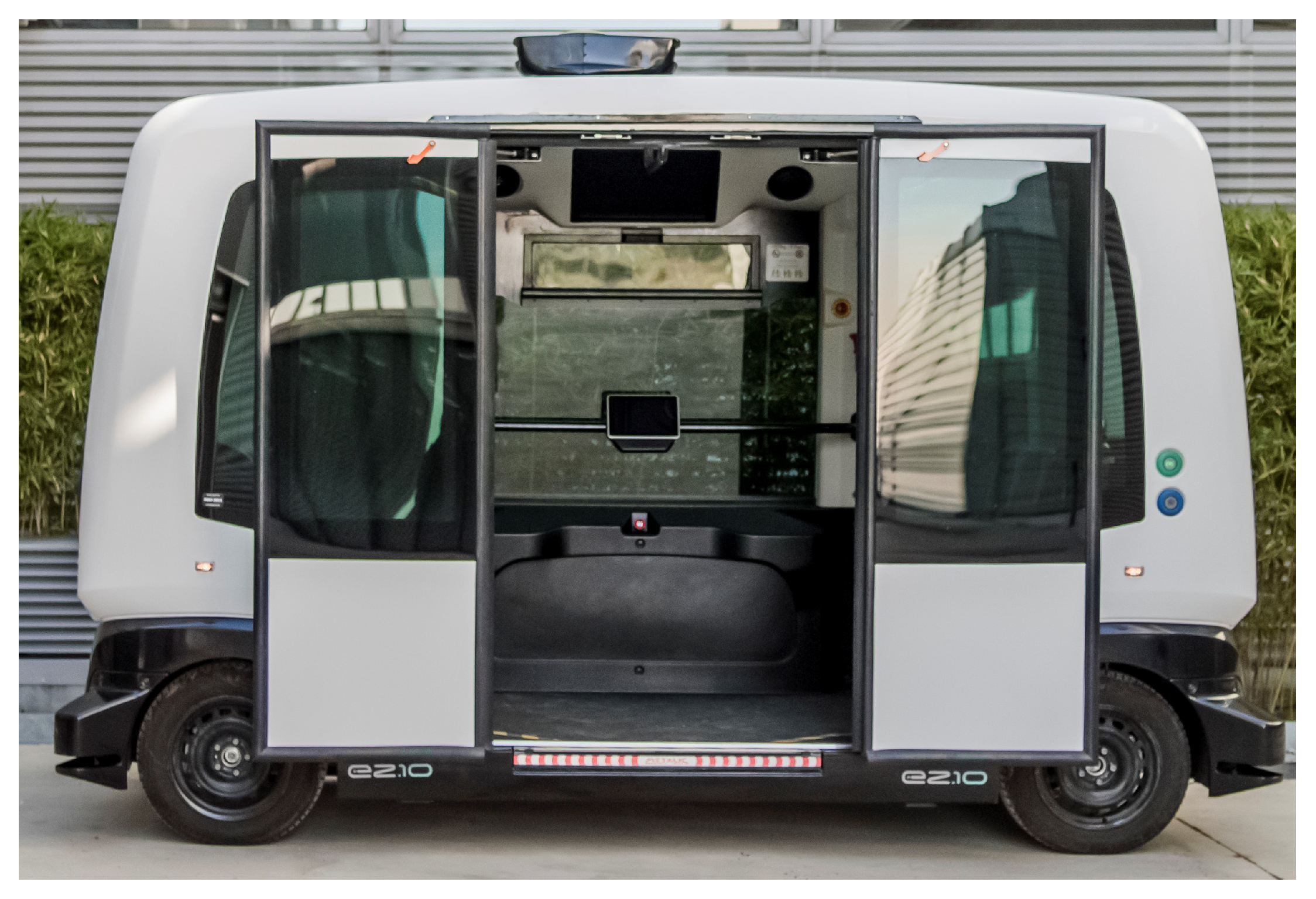
The goal of this paper is to place into context those problems and approaches proposed to solve some of the challenges that are derived from Intelligent Transportation Systems outside of the normal traffic flow and restricted traffic locations, such as protected places, airports, business centres, etc. Hence, this work is the culmination and full revision of the state of the art paradigms, approaches and algorithms that are taken into account and implemented to demonstrate the validity of such methods in non-standard environments where sensor errors readings, poor localization, hard terrain navigation, wildlife detection or unpredictable weather changes have to be overcome. For this reason, among other mechanical and electrical challenges, this paper is focused on solving problems related to localization, perception, mapping, planning, human-machine interaction, software architecture and cybersecurity. All of these problems are solved but not fully optimized because it is not the final goal of this work. Moreover, all the systems have been tested in different track tests with narrow corridors and sinusoidal roads with heavy slopes in both simulated and real environments. The immediate application is based on a technological demonstration which consist of a prototype as a rough example of what can be achieved in these kinds of environments where the fundamental task of the vehicle is to transport people from the starting point to the endpoint without human intervention. In order to demonstrate the methods proposed and the integration between all of them, the research platform selected is a LIGIER vehicle similar to WEpod used in [
5] EZ-10 from 2014.
On the one hand, the software architecture deployed in this vehicle is based on the iCab [
6], where all the nodes involved are in charge of solving specific problems with the aid of a set of managers that analyze the vehicle information and select the most suitable outputs for the best performance based on several metrics. These managers are in charge, for instance, of allowing the vehicle movement or selecting which control method is better to use for specific situations. These items are the key to the integration and functionality of the platform, allowing redundant problem solving with different algorithms and the integration of the solutions computed within the whole system. On the other hand and, out of the scope of this work, there is a remarkable point related to the scalability of this manager paradigm that can be discussed: Since this approach is based on a collaborative set of modules, it is always conceivable, through the implementation of several basic changes, to adapt and improve the system for different applications or new features in the near future with little effort. However, as stated, this is something that is considered outside of the scope of this paper.
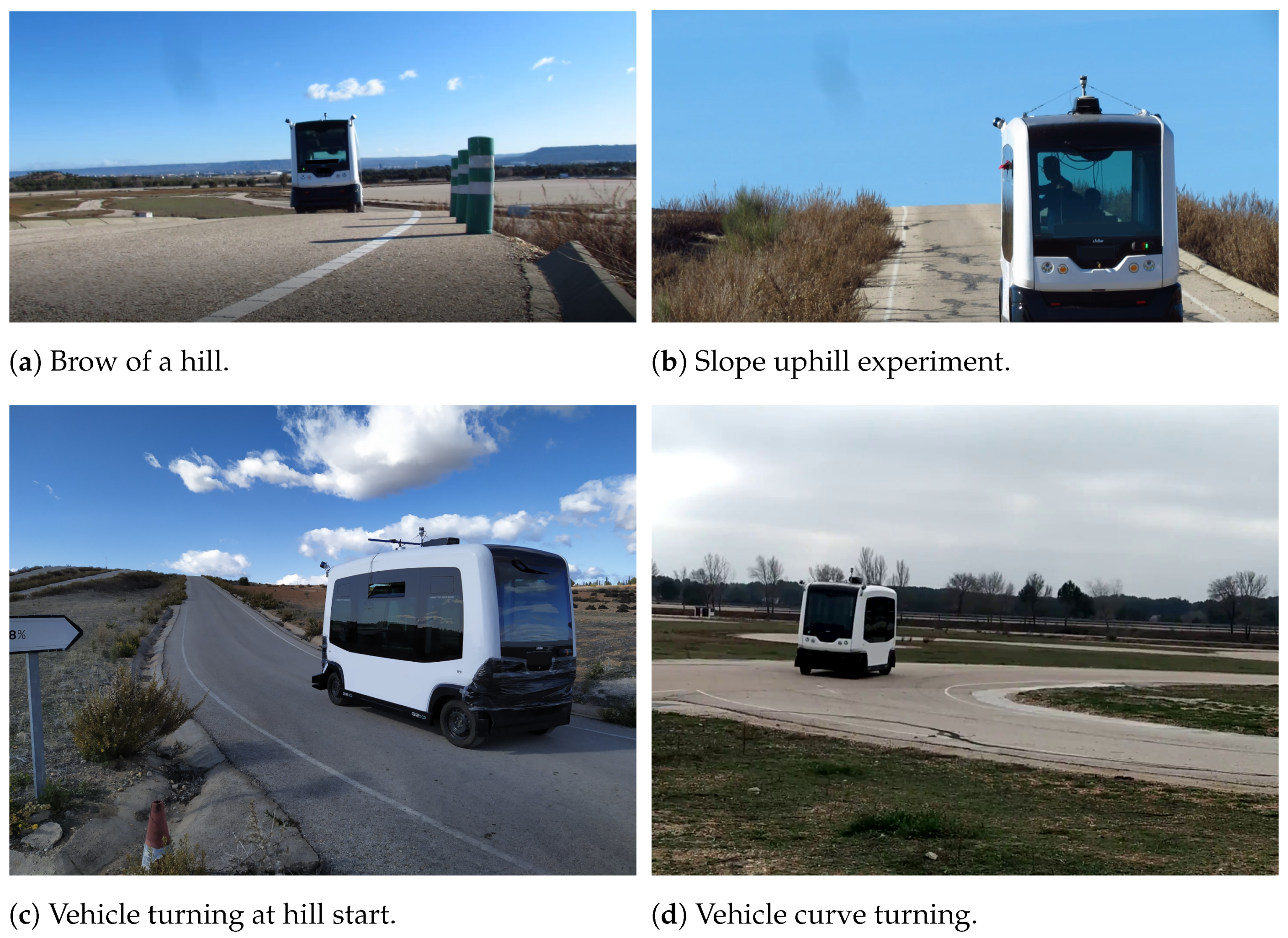
Furthermore, the environment where the vehicle tests its performance is a road well-formed in an unstructured environment with hard slopes, narrow spaces to navigate and sharp curves. The start and end points are always the same and the vehicle performs the same path repeatedly. The road has no marks and there are no steps between the road and the ground; sometimes the path leads to a walled mountain and sometimes there is a ravine with no protection at all; hence, the vehicle needs to deal with a rough environment full of potential dangerous zones. Therefore, taking all of this into consideration, the main idea is that the vehicle should perform a complete tour with passengers while always keeping in mind their comfort and security, adjusting the speed and performing some tourist stops known as Points of Interest (POI), in which some audiovisual material to improve the experience will be shown. All of this is to occur while the system is tracking possible obstacles en route, adjusting its speed to avoid collision or enabling cruise control and controlling the platform’s low-level mechanisms to traverse the stipulated path.
Hence, to summarize, the contribution of this paper is the integration and validation of accepted solutions for localization, lateral and longitudinal control, perception, mapping, self-awareness and cybersecurity. All of them are able to work concurrently in a robust software architecture able to recover from errors, with the integration of the novel idea of managers in charge of adapting each decision on the road to cope with real-time events.
2. Vehicle
The selected vehicle for this work is a 2014 EZ-10 model from LIGIER. The vehicle, which can be seen in
Figure 1, is an electrical shuttle that carries up to 12 passengers. The platform integrates its own low-level control based on a double Ackermann geometry that improves maneuverability in narrow spaces. Nevertheless, it must be clarified that this low-level control only generates the proper signals to produce the speed, acceleration and steering angle commands sent by the high-level control interface implemented in this work to govern the vehicle.
On the other hand, these kinds of shuttles have been used in other research but only tested in the face of urban and structured environments. For this reason, important questions that this work proposed include the following: if the vehicle software deployed is able to fulfill all the use case requirements established to properly work; if the vehicle itself, mechanically and electronically, is able to cope with rough and hard environments; if there exists a problem between hardware and software design limitations; and, if so, how will the problem affect the overall performance of the system behaviour. Thus, from the project and work perspective, this low-level control was verified and tested properly before adding any software and it was decided to maintain the vehicle basic capabilities separate from the high-level architecture.
2.1. Devices
To fulfill the requirements of the proposed application, the devices added to the initial platform were selected after an intense study case in a simulation environment and, unfortunately, this goes out of the scope of this work and, in order to be as succinct as possible, it will not be discussed in this paper. From the set of sensors proposed and accepted for system, there are a total of three LiDAR sensors: one of 64 layers on the top of the vehicle and two of 16 layers, each one in the frontal corners with a specific angle position to cover the frontal environment and the surroundings. For the localisation module, the device used is Novatel-GPS-702-gg and the Novatel Flexpak6 is used for differential corrections DGPS. Finally, the IMU used is a Pixhawk module PX4 version 2 capable of providing orientation and angular velocity readings. In this manner, all these sensors in conjunction provide a proper solution for the vehicle localization capabilities and the road/obstacle detection processing.
However, there is a topic related with these sensors that has to be taken into account with respect to the kind of environment the platform is working in. Since the platform copse with rough terrains, strong winds, dust clouds and wet or cloudy weather can damage the sensors and will introduce errors in their readings or several malfunction problems. For this reason, the sensors that work outside the vehicle must be protected with strong supports and periodic maintenance to test its integrity and proper behaviour, which is something this work tries to accomplished at both hardware (adding new supports and structures) and software levels (see
Section 3.7 for more details).
Along with the sensors, the main CPU power load is provided by a computer with an internal GPU and i7-8th gen core for LiDAR Point Cloud processing, while the control and mission modules run in a NUC computer along with the CAN bus interface. In addition, both computers are in the same network segment as the LiDAR and GPS sensors. Finally, the electric supply for the computers and sensors has been obtained from 12 V and 24 V batteries with its corresponding power support devices to maintain the specific demand in the case of voltage fluctuations.
3. Software Architecture
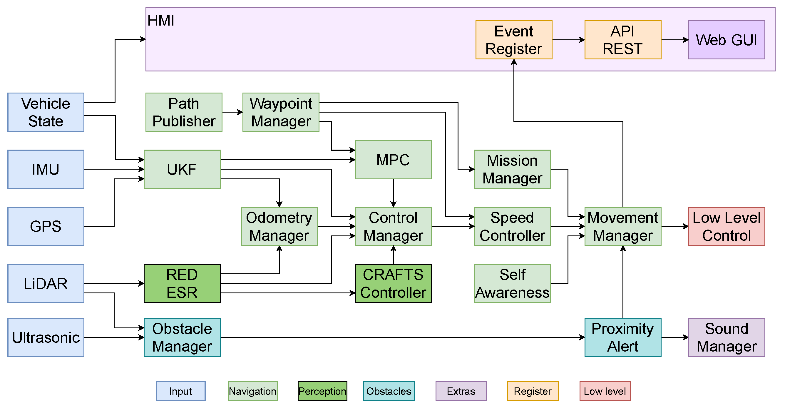
Figure 2 shows the workflow of the system. The information acquired from the sensors is transformed and fed into the processing nodes, then the filtered and sensor data is used to generate proper solutions dependent on the environment and the vehicle situation on the road. After these processes are completed, all the information is sent to the managers and, as a final step, the control commands for the low-level controller are generated to move the platform. It is necessary to remark the importance of the managers in the system to allow or select which traffic/sensor information will be used. Although some nodes are always generating the control information, the managers allows the forwarding of the control commands to the lower level only if several conditions are fulfilled; these conditions depend on the solutions established, computed and confirmed by each system node assigned to a specific task. For example, the Odometry manager decides which control is in charge of vehicle movement, which is either the MPC (Model Predictive Controller) or the Reactive Road Controller, and their actuation will depend on the degree of trust (Score) the system computes from sensor data. This paradigm of workflow is used for decision making within the system for the vehicle to decide the methods for controlling the platform depending on the situation.
The following sections will describe the solution proposed for each problem that has arisen during the project lifetime and each manager node used to generate a proper traffic/information flow downstream to the final control command in real-time.
3.1. Localization
The nature of the environment where the driverless vehicle has been tested includes the absence of building surround it as it is not urban and a clear and visible sky is present almost all along the route. Those characteristics meet perfectly with the use of a GNSS based localization since high obstacles do not cover satellite signals. Other absolute localization methods based on LiDAR, such as Adaptive Monte Carlo Localization (AMCL) [
7] or both, LiDAR and GNNS as in [
8], are not suitable for this project. A map full of features that can be matched with LiDAR sensors necessary for those kinds of algorithms cannot be generated due to the absence of obstacles and most of the features that can be found are due to vegetation, which changes through time.
The above mentioned motivates the use of a high precision GNSS receiver as the main global localization source described in
Section 2.1.
To improve the localization accuracy, many GNNS receivers include the possibility of receiving satellite signal corrections called real-time Kinematic (RTK) corrections from Networked Transport of RTCM via Internet Protocol (NTRIP). The receiver is configured to connect the nearest NTRIP caster and sends periodically the GNNS status via NMEA protocol and the caster returns corrections in RTCM3 format. When corrections are received, the receiver recalculates the position, improving it significantly from a covariance of around 0.5 m in X/Y axis to a covariance of m.
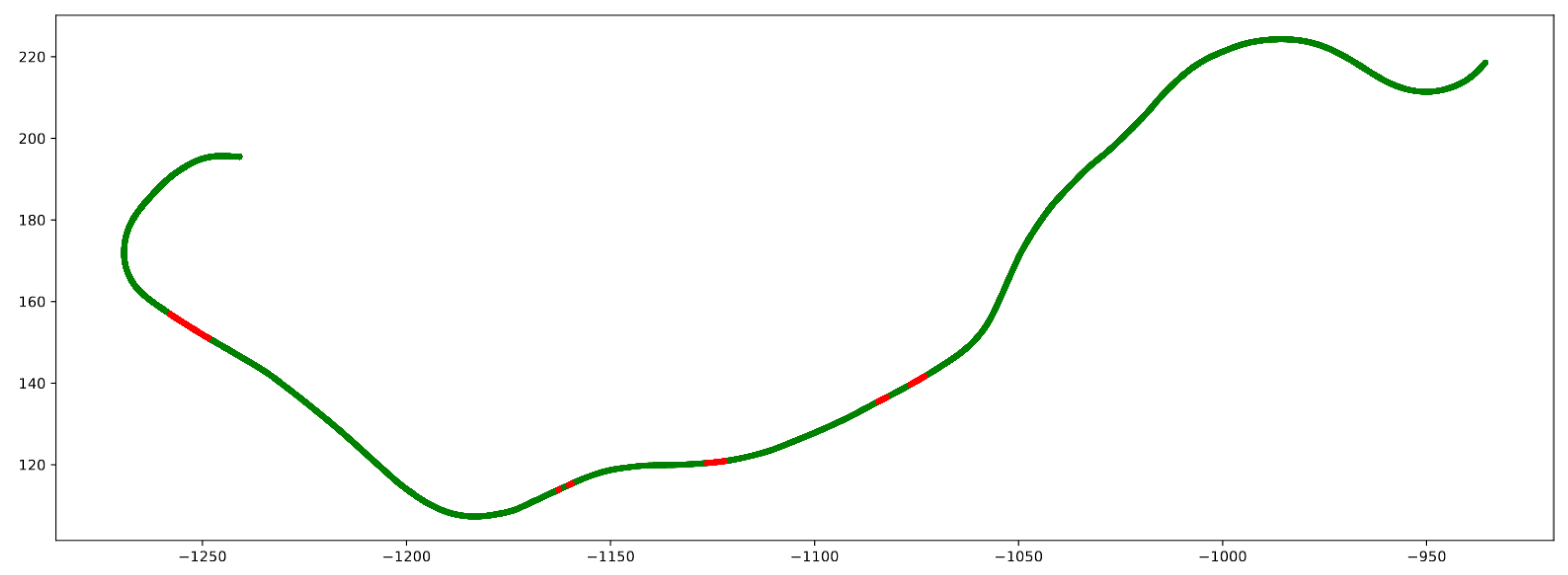
The drawback of this localization resides in the dependence of network connection at every position, which is evaluated at every point of the route in this project. In order to produce that, all the route positions are recorded along with the internet status determined by the ability to ping a specific caster IP address. The results show an almost full internet connection during the route (95%), with exception of some small areas where the connection is lost, as shown in
Figure 3.
However, those small areas are not a big issue as when the internet connection is lost since it can be detected where the covariance increases, which is the moment when the reactive road controller starts to work.
3.1.1. Unscented Kalman Filter (UKF)
The Kalman filter is commonly used in mobile robots localization as it can fuse different odometries and, as a result, provides a more accurate one. Different variations of the original Kalman filter can be found in the literature; however, for this project, the Unscented Kalman filter (UKF) is used as it can handle non-linearities of the system in the filtering process [
9]. The software used in this project is a ROS implementation of the UKF [
10], which can filter an arbitrary number of odometry sources.
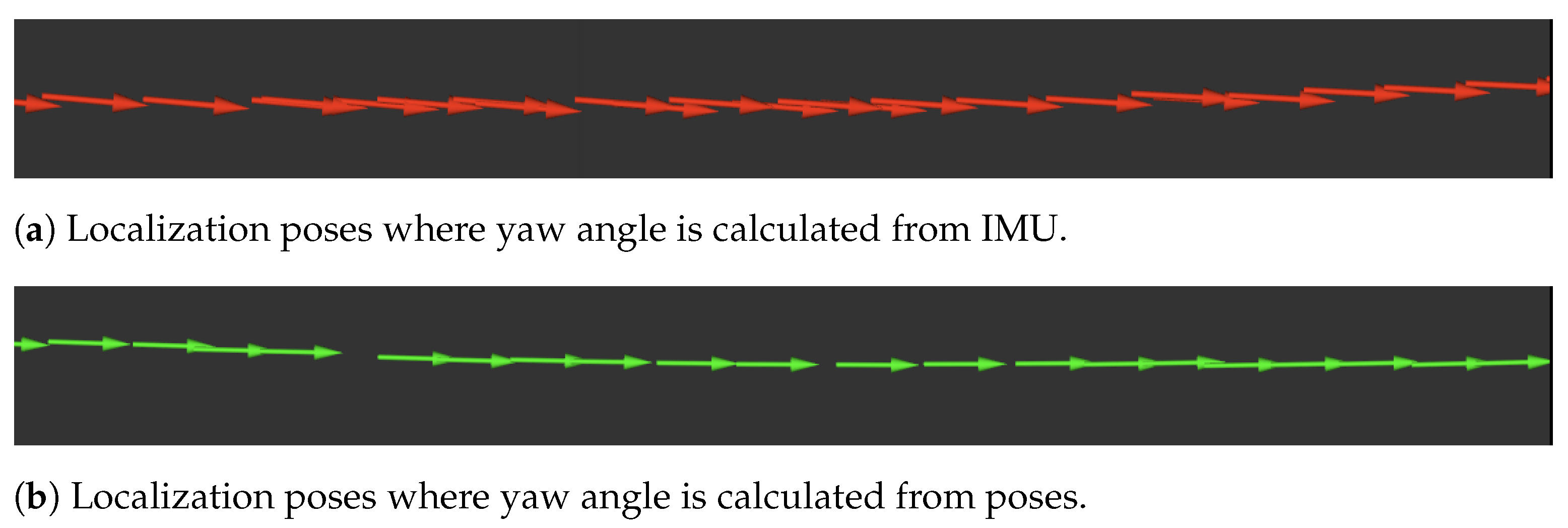
Together with position, a reliable orientation is essential for good control of the vehicle. The use of an Inertial Measurement Unit (IMU) can improve the UKF fusion by including rotation speeds and linear accelerations. High-performance IMU usually includes a magnetometer sensor that can provide orientation information by measuring the Earth’s magnetic field. However, magnetometers need a good calibration that is usually performed by turning the sensor attached to the vehicle in different directions. The impossibility of performing that with the project’s vehicle due to its high weight results in poor calibration of the sensor and, consequently, a low accuracy of the yaw angle measure that adds a random offset to the angles as shown in
Figure 4a. On the other hand pitch and roll angles are stable as they do not depend on magnetometer and those angles are used in the UKF.
Due to the inaccurate yaw angle provided by the IMU sensor and the high accuracy of the GNSS position, the orientation is calculated using the current and last received position that is at a distance of
d meters. The yaaw angle
is calculated as:
where
and
are the
X and
Y coordinates increments of two consecutive positions separated
d meters,
is the current speed,
and
are the current and last position yaw angles and
is the taw rate. Its covariance
, needed by the UKF is given by:
where
and
are the current
X/
Y position covariance and
and
are the the last position covariances.
The proposed orientation calculation provides good results and outperforms the angle provided by the IMU sensor as shown in
Figure 4, where the yaw angle from the IMU sensor has an offset compared to the one calculated from poses which is more coherent for the vehicle used in the project. As with position, this angle accuracy highly relies on the NTRIP corrections but, similar with position, if covariance increases then the secondary navigation algorithm overrides the control.
The last source of odometry included on the Kalman Filter is the wheel odometry. This odometry is based on the wheels velocity and steering angle provided by the vehicle’s CAN-BUS. The data are used to estimate the vehicle displacement using a kinematic bicycle model where the increments of
X and
Y coordinates (
and
) and yaw (
) are provided by:
where
is the steering angle,
determines the position of the vehicle centre of gravity (0 in the front and 1 in the back wheels) and
is the wheelbase of the vehicle. The calculated wheel odometry accumulates are derived over time and thus only position, orientation increments and speed are considered. The addition of this information to the filter provides a stable odometry source that improves its performance.
3.1.2. Odometry Manager
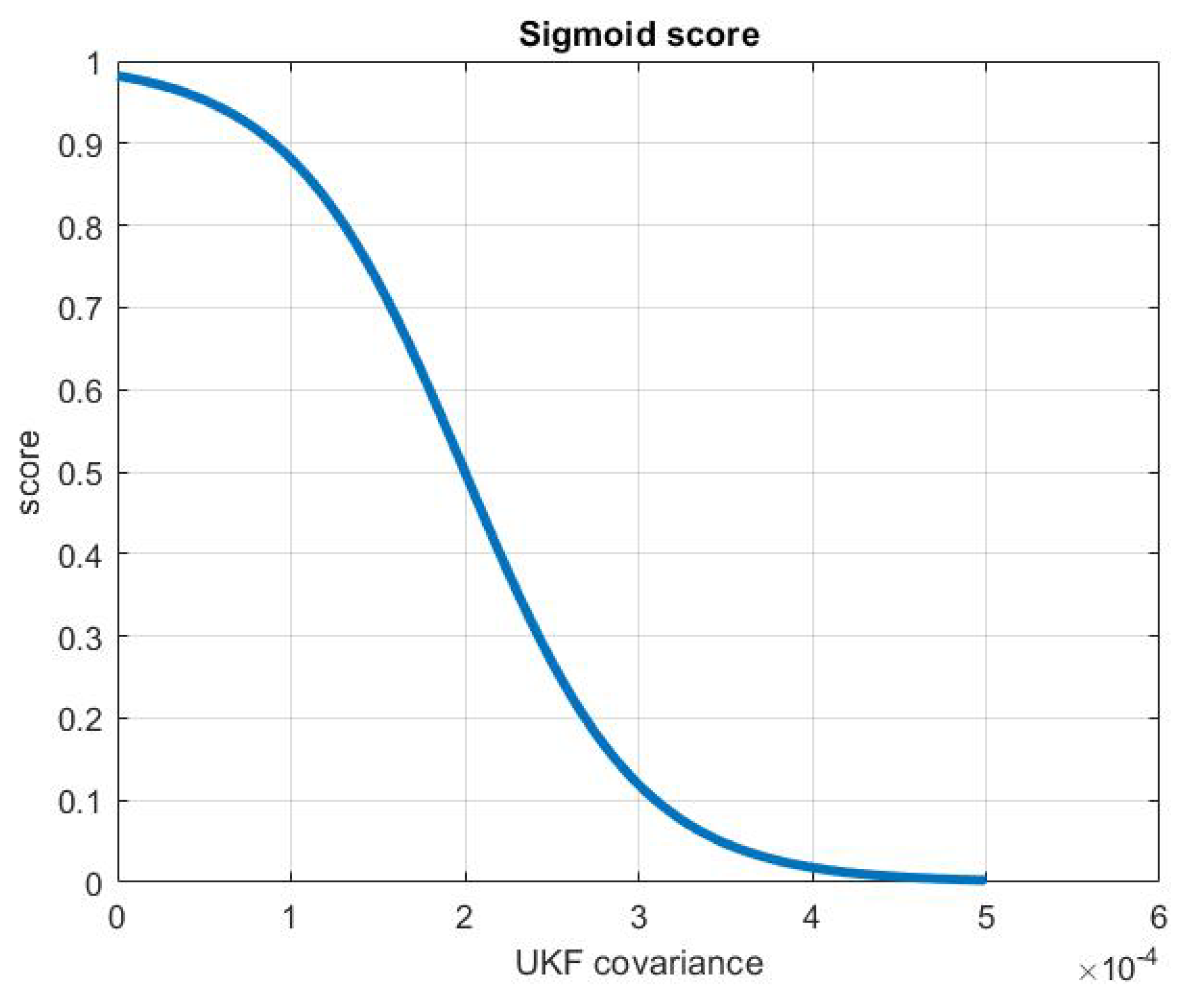
This module is in charge to analyze the odometry provided by the localization package. The input is taking into consideration the covariance of the UKF output and providing a simple score showed in
Figure 5. The score is generated with the sigmoid formula (
6) where the values
a,
b and
c are the result of experimental analysis where the covariance and uncertainty start rising due to different factors such as DGPS lost signal, 4G lost signal, IMU interference and noises. The score value generated is used later to select which type of control will be used and is based on localization or the reactive one based on road detection.
3.2. Path Manager
The operational design for this specific application is the repetition of the same travel repeatedly. Due to these constraints, the global path is always static and the problem is solved by using a smooth path the vehicle should follow. After working with big distances and, consequently, with a big set of waypoints, it was required to change the search method to find the nearest waypoint accessible for the vehicle. Since the conventional stochastic search methods decrease the performance and increases the CPU load exponentially with a big number of samples, alternative kind of search methods and structures are necessary to be applied in this type of situation for improving performance and scalability. As a consequence, the method used for this task is a KDTree search structure [
11].
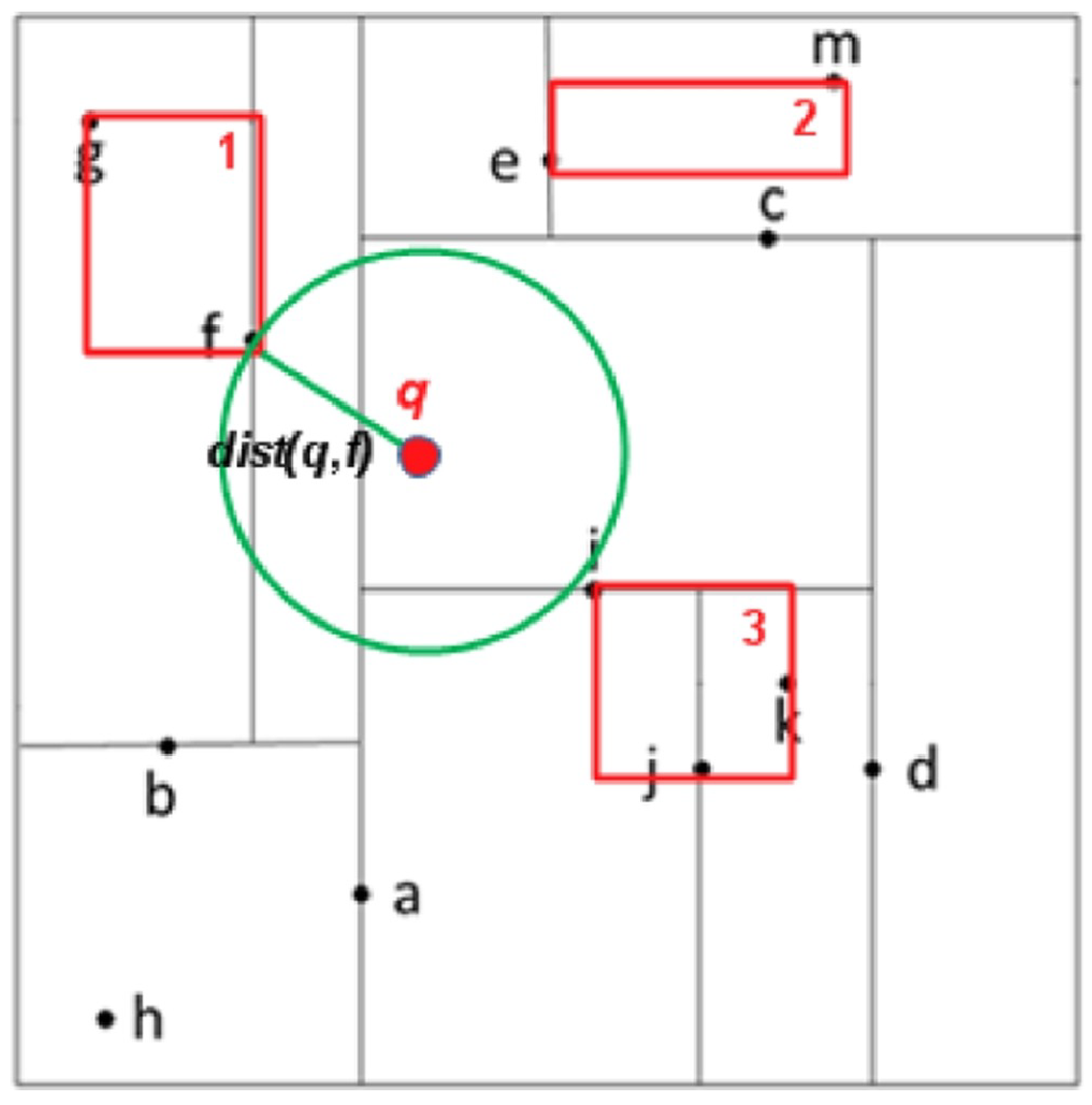
The search space is the feasible region of the space in which the set of all possible solutions is defined. The search space of this work is based on the space partitioning made by a KDtree structure (
Figure 6 for which its nodes take the form
(represented as
a,
b,
c, etc.) The square shapes in red represents the distance between the nodes and the circular green shape is the search radius from the starting node. As previously stated, the node information is extracted from a pre-computed path that tracks every position traversed by the real vehicle. Hence, each node represents the configuration of a rigid body in 3D by four degrees of freedom: Three translational
and one rotational
, extracted from the quaternion representation of the pose orientation [
12] and computed from the vector between two adjacent path poses. Taking into account the real usage of this approach, the space dimensions are reduced from six to four degrees of freedom since the system is only interested in the position and orientation of the vehicle on the Z axis; therefore, there is no sense of measuring the roll
magnitude on a vector and the pitch
has no impact in the search process within this environment.
As a brief explanation of its functionalities, it must be said that the Path Manager module provides support for any other architecture node that needs path information. Its core task can be seen in
Figure 6. Each odometry reading (red point (q)) is processed to compute the nearest path pose by extracting all potential pose neighbours that lies within the radius of a circular search area (green circle). The computed result(s), the one(s) nearer to the current vehicle pose to the path (black point f in this case), are fed into the MPC controller (see
Section 3.6.1 for more information) that will then be in charge of following the pre-computed path.
3.3. Mission Manager
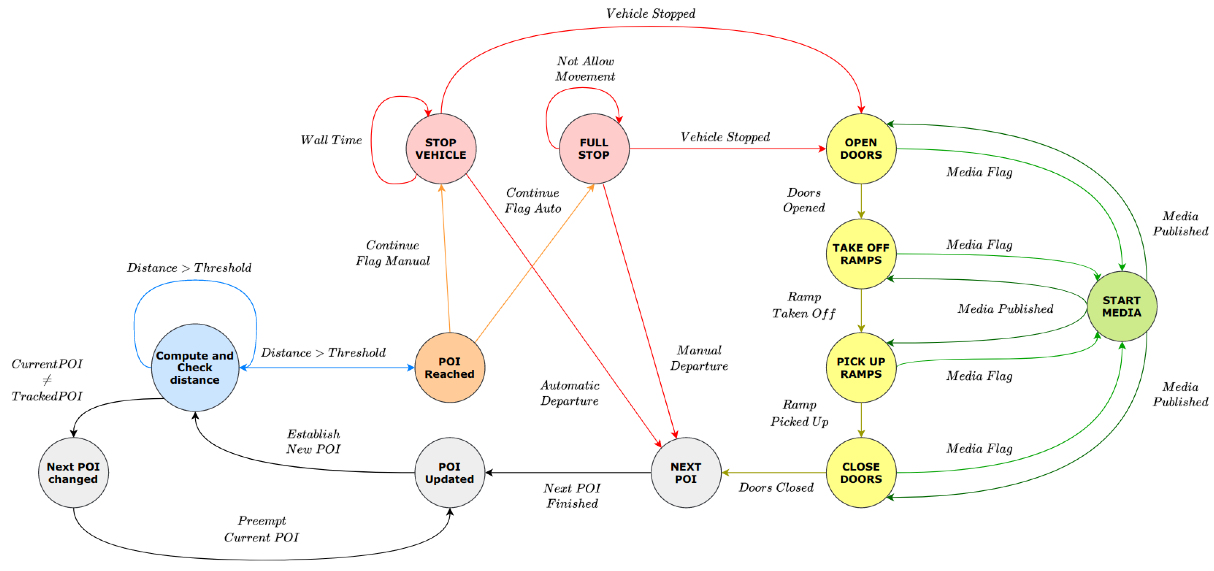
There are certain moments in which the high-level control of the platform must decide which course of action to take in order to complete several tasks in route. These points in which the vehicle is going to decide what to perform are called POIs (Points of Interest) and they are distributed along the global path on the platform that the vehicle will traverse. The module in charge of this task is the Mission Manager module and it is implemented with the framework of action-lib, which is a stack that provides a standardized interface for interfacing with pre-emptable tasks. This stack is based on a Client-Server architecture in which the client defines a goal, the server processes a set of actions to perform during the goal processing and feedback is reported to the client to supervise at every moment in terms of what the inner state of goal processing is. In this manner, a high-level task manager is implemented allowing the platform to decide at specific moments which tasks must be performed when the vehicle is on the route.
The goal in this particular case is defined in two steps: The first step is reaching a POI, that is, the distance between the platform and the POI must be near an arbitrary threshold and the second step starts once the platform reaches the specific POI position, in which a state machine is launched to perform the set of actions the vehicle must perform for this POI.
Figure 7 shows a naive implementation of a possible state machine for the vehicle used in this research.
What the states mean:
STOP: Stops the vehicle and pass control to the speed controller to stop on POI;
FULL_STOP: Stops vehicle and pass control to movement manager to stop on intersections;
OPENNING_DOORS: Open vehicle doors when the vehicle is stopped;
TAKEOFF_RAMP: Take off the vehicle ramp when doors are opened;
PICKUP_RAMP: Pick up the ramp when the ramp is extended;
CLOSING_DOORS: Close the door when the entrance is clear;
NEXT_POI: Proceed to the next POI once the current POI finishes its processing;
START_MEDIA: Send confirmation to high-level control to start a multimedia file in the passenger GUI.
3.4. Perception
The understanding/interpretation of the traffic scene, in which a moving vehicle is located, is a complex objective and inevitably requires an advanced inference process. It must begin with a reliable perception of the various agents that are part of the scene (vehicles, pedestrians, etc.) as well as the characteristics of the infrastructure in which the vehicle moves (road limits, the geometry of the intersections, etc.). For these reasons, the problem has been dealt with using Computer Vision and LiDAR Technology approaches resulting in proposals of various kinds.
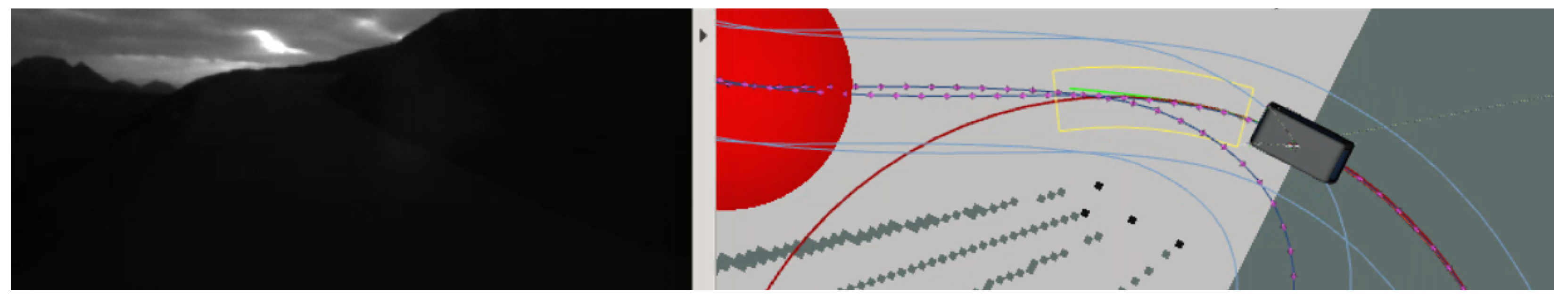
There is a concern about the lack of use of cameras in the platform. The decision to use the only LiDAR for perception resides in the possibility to work in dark environments (
Figure 8) where the mounted camera is not optimal.
3.4.1. Calibration
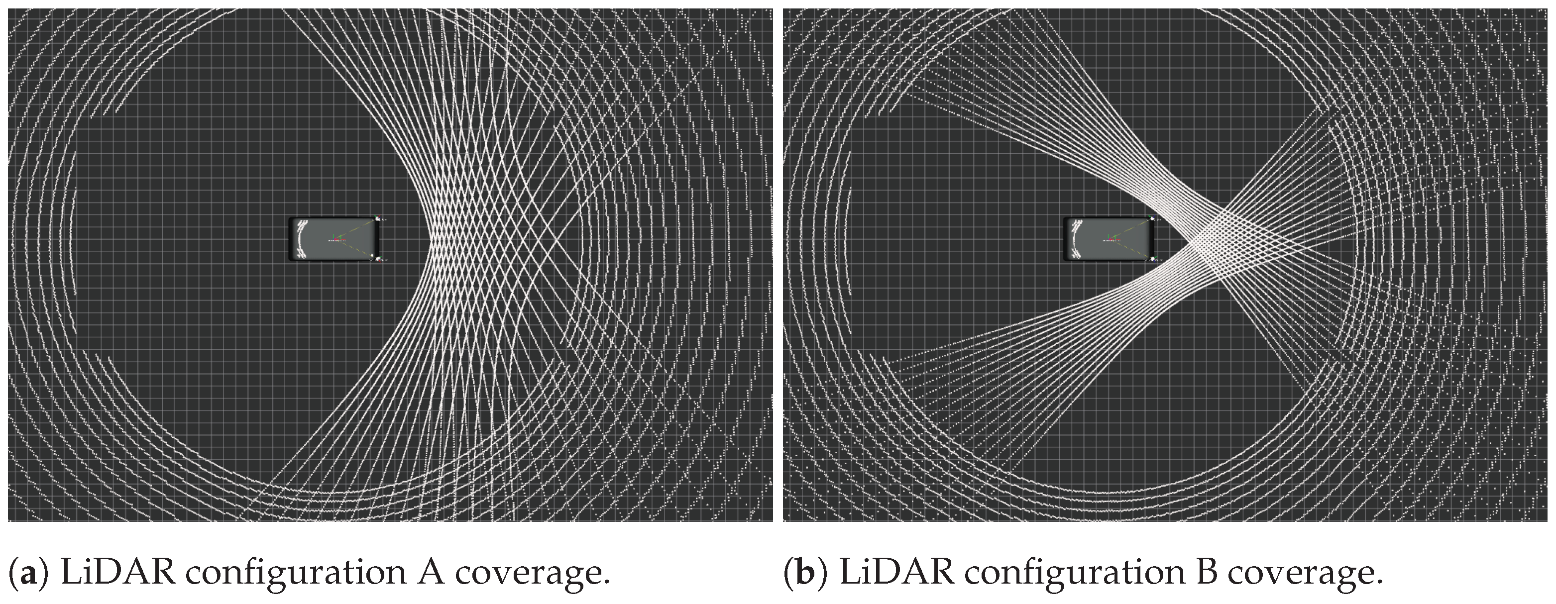
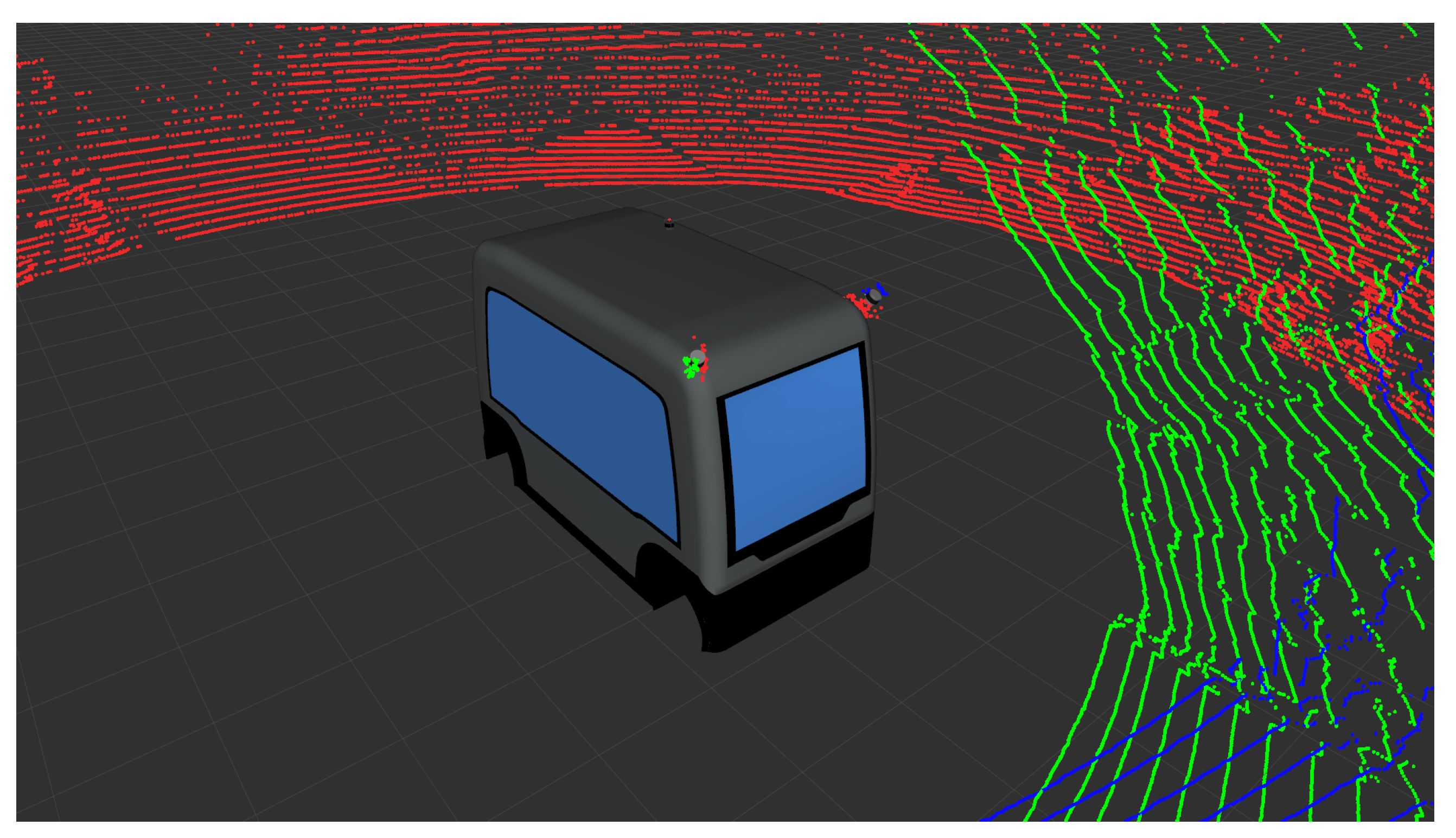
To detect the environment, a LiDAR sensor of 64 layers with a complete vision of 360 degrees was mounted on the roof of the vehicle. The device was lifted 34 cm to optimiee the maximum ring layer hitting the ground and avoiding as much as possible any point that will lay inside the roof of the platform. Additionally, two LiDAR of 16 layers were mounted in front of the vehicle with specific angles to cover the blind spots and to detect the road and the critical obstacles near the platform.
Figure 9a shows the final distribution of the LiDAR 16 and 64 with the coverage in front of the vehicle.
Figure 9b shows the initial alternative discarded for poor environment coverage and lack of road boundaries detection with bigger blind spots.
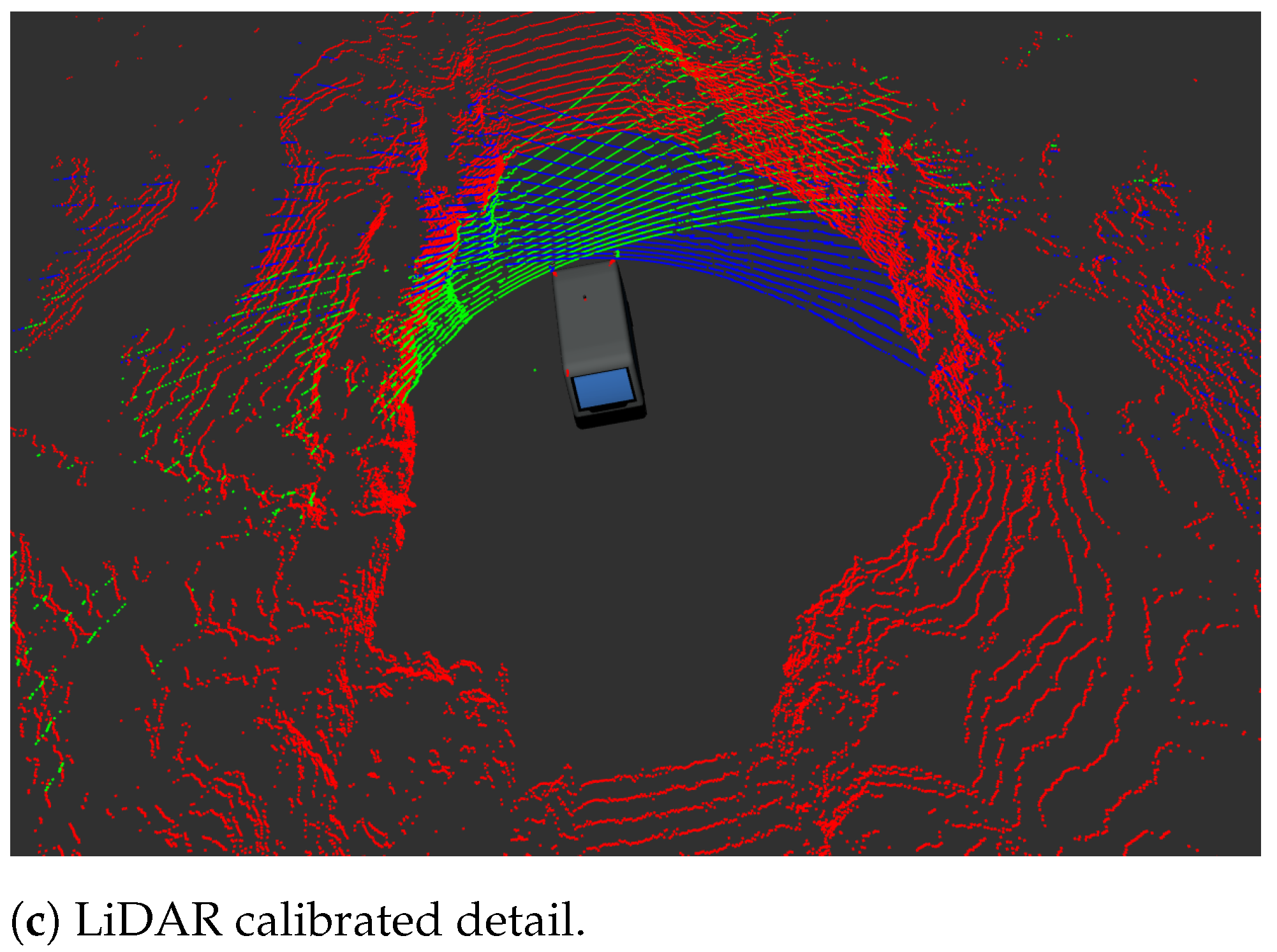
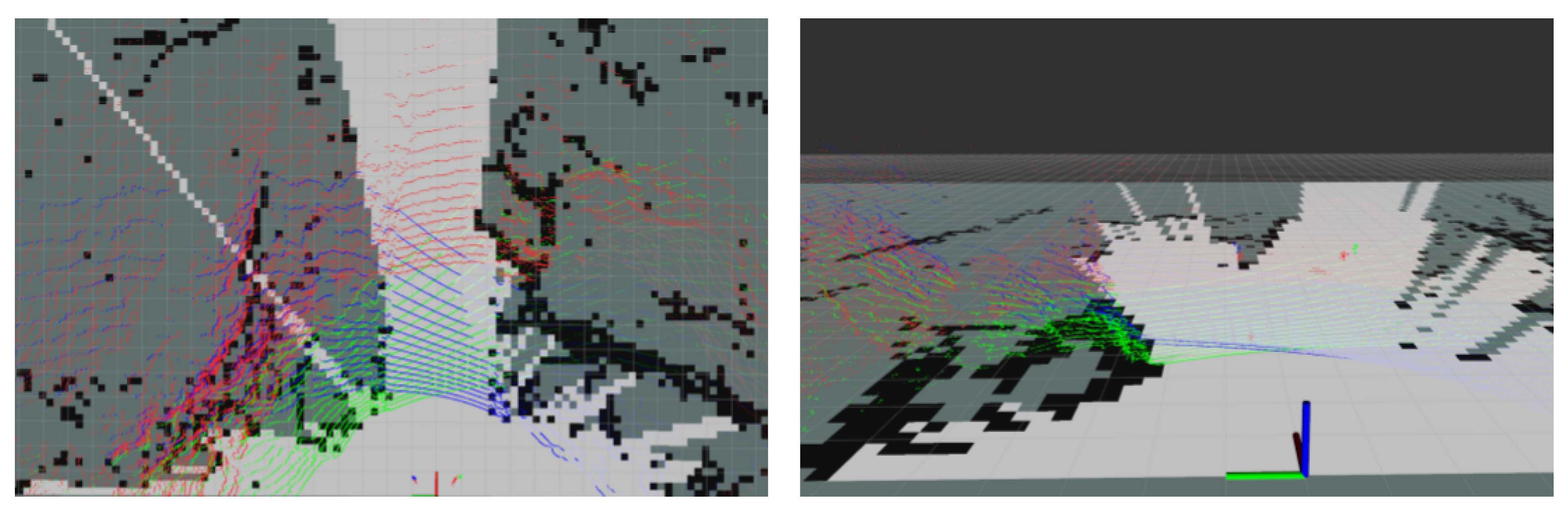
One of the main problems using three LiDAR sensors is the extrinsic calibration stage. All the LiDAR must detect, measure and show the same distance to the same set of obstacles. In the literature, some automatic method was developed for this task such as the work of pairing stereo camera and LiDAR or directly pairing LiDARs. For the initial stage of extrinsic calibration, the method of Guindel [
13] has been used in the LiDAR variant. The result has been tested in an industrial warehouse with three walls and the floor. With a little tuning, the final output of the whole process has been proven to be optimal enough as observed in
Figure 9c. Furthermore, it is possible to appreciate the shared space of the LiDAR sensors on the floor or by pairs in the sides.
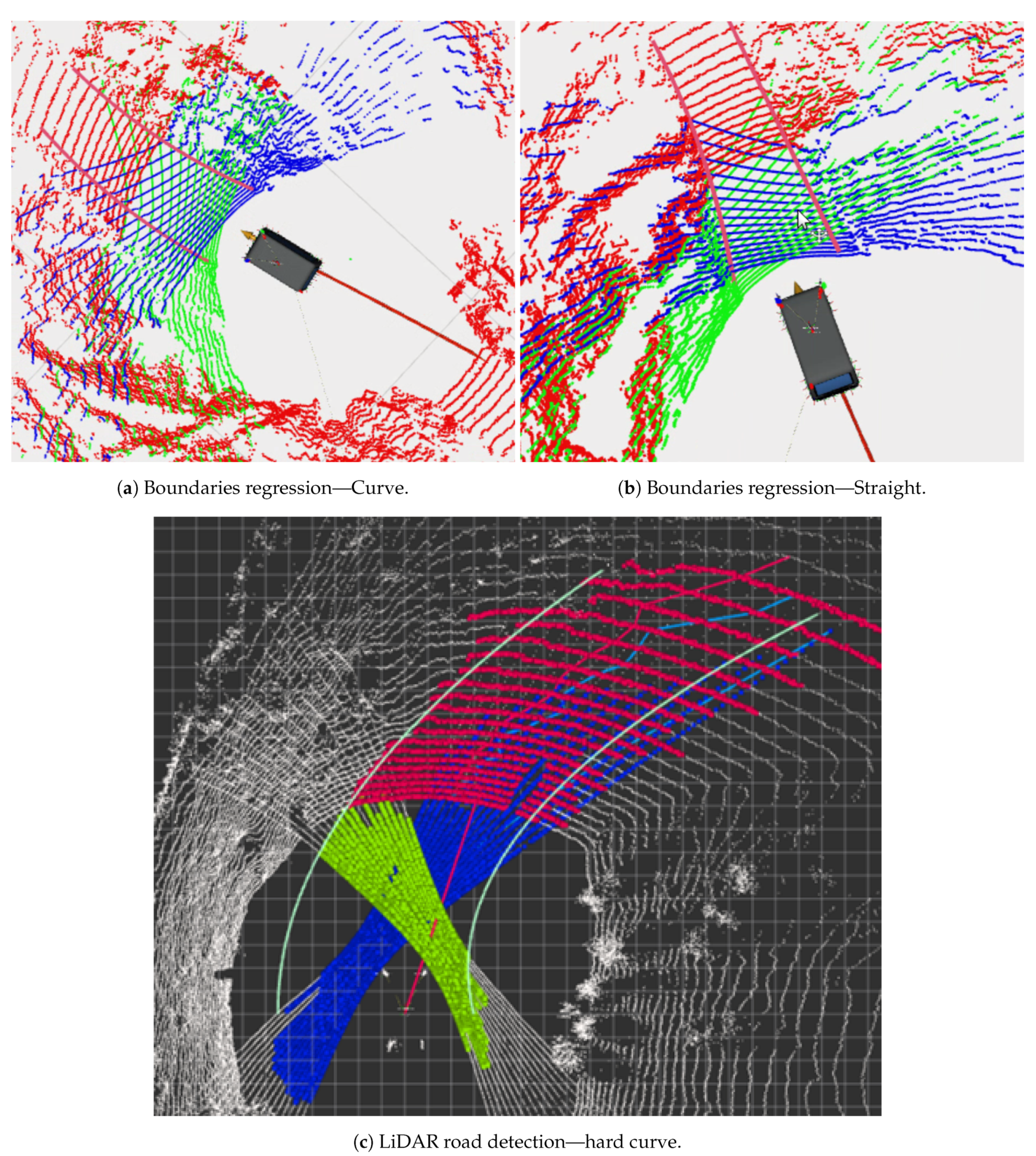
3.4.2. Road Detection
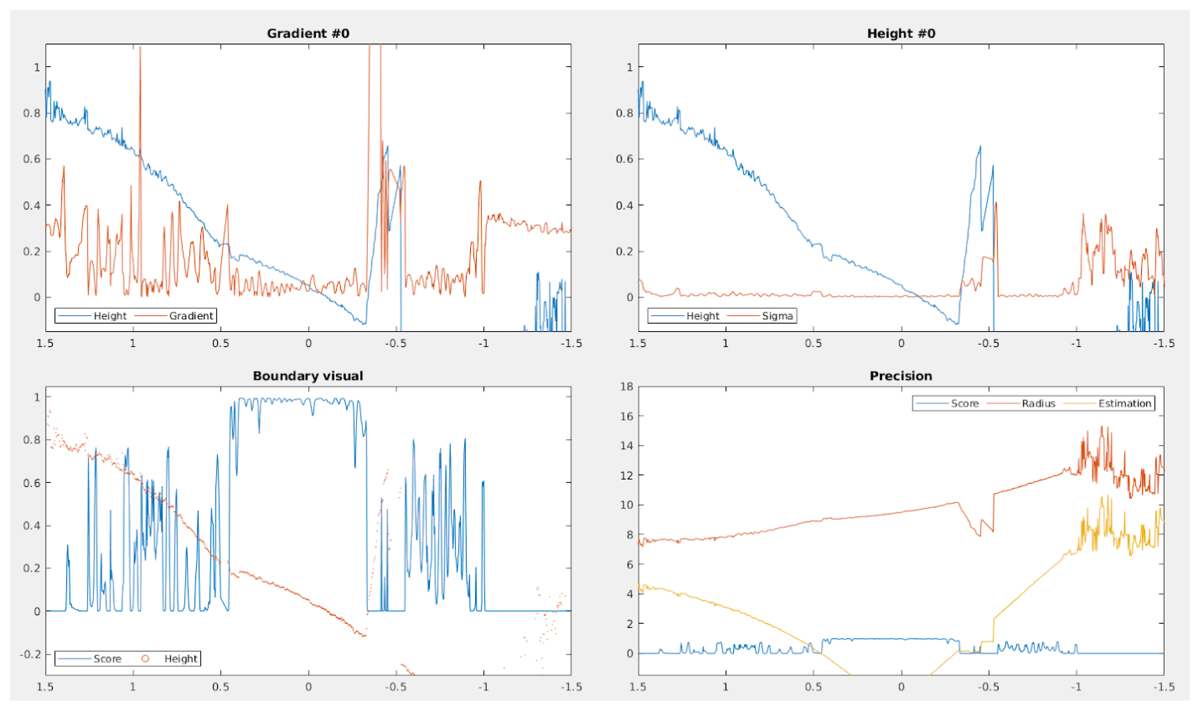
Due to the lack of 4G and GPS signal in some areas of the route, it is mandatory to count on a backup system that switches between the localization and odometry control process to a reactive control strategy to maintain the vehicle inside the road. Therefore, apart from the standard odometry control, the system also relies on the road detection node. This node implements a probabilistic model to detect the road boundaries left and right. Thus, in this environment, the most important challenge is to detect and extract the exact points of the road boundaries when there are no marks, signals or boundary steps that are usually found in urban areas. The method processes separate nodes and PointCloud readings of each LiDAR and then each PointCloud is integrated and transformed into rings used to search sequentially the road limits, Finally, with the boundaries computed, the road is modeled with a mean-square fit. This method aims to identify the navigable space based on the analysis of first and second derivatives of the road height in two iterations. In the first iteration, a window operator is used over the rings extracted and this takes the geometric characteristics of each road point computed and assigns a score that represents the likelihood of being part of the road. With this set of points and scores, the search gives a new score to each LiDAR ring selected that will be used later to extract the left and right road boundaries.
This score
(
7) is a sigmoid function based on the gradient ∇ (
8) of the height, the sigma
(
9) value, which is the relative height based on the medium deviation, and, finally, the estimation of euclidean distance
(
10) to the limit of the road based on the last PointCloud. To obtain those values, the neighbour operator is used. This operator is the group of adjacent points to the analyzed point. Each
is calculated individually based on slopes, curves and smooth paths to obtain the best results.
The neighbours
j are selected based on the left or right side of the reference point inside of the road. The reference point is calculated using the normalised azimuth subtraction
Algorithm 1 and solves the problem where the neighbours belong to different sectors (i.e., inside or outside of the road).
| Algorithm 1 Normalized azimuth subtraction. |
Input:,
Output:
Initialisation: - 1:
ifthen - 2:
return - 3:
else ifthen - 4:
return - 5:
else ifthen - 6:
return - 7:
else - 8:
return - 9:
end if
|
The top left of
Figure 10 shows the gradient in height of the data information for only one ring. In the top right, the sigma value is the relative height based on the medium deviation of the previous data for the same ring and by taking into account the displacement. The bottom left indicates the score. Finally, the bottom right shows the precision of the score based on the estimation of the regression with neighbours.
In the second iteration, with the boundaries already computed, this method generates a 2D model of the road with a mean-square fit that uses the selected scored points for each ring (taking into account a threshold) as a regression method to extract the road limits. This regression is performed in two steps to provide more accuracy: the first step computes a rough draft of the road limits and then, the second step applies a filter to smooth the curve and extract the outliers. In this manner, the road boundaries extracted can determine the position of the vehicle in the road and, therefore, it is possible to generate the lateral control commands to drive the vehicle inside the road bearing in mind the solutions provided by the detection algorithm. The method proposed for road detection works with straight and curved roads (
Figure 11a,b) determining the navigable space for the vehicle (
Figure 11).
Thus, with this process, the vehicle is able to generate each road boundary, which are used in the next steps to compute the line that describes the middle of the road. This last solution is the trajectory that will be followed by the vehicle reactive control when sensor data are not good enough for the system to be controlled purely with odometry information.
3.5. Mapping
In order to navigate in a safe manner, the vehicle generates a local occupancy grid map, which represents the free (drivable) area and the obstacles present around the vehicle. This map is obtained by combining the point cloud data from the LiDAR sensors, which is previously filtered to avoid false detections and to make it more robust overall. Afterwards, the local map is analyzed to determine which obstacles might pose a threat to the vehicle and by considering its current trajectory. Finally, the extracted information is used to send the corresponding control signals to slow down or stop the vehicle in order to avoid any possible threat.
3.5.1. PCL Filtering
One small problem using LiDAR in the platform is to optimize the position to balance the rings hitting the vehicle versus the height position in the roof and blind spots in the surroundings. Consequently, there are some auto-hits of the lower rings in the corners of the vehicle and some laser collisions in other LiDAR devices, as can be observed in
Figure 12. The solution proposed results in the use of a filter with the shape of the platform to erase undesired points in the final point cloud. Moreover, sometimes the LiDAR sensors may have false positives and present random points in front of the sensor due to systematic errors, interference or fog. For this reason, an additional filter is applied to the point cloud in the critical area near the vehicle in order to avoid processing those ghost points and detecting them as obstacles in front of the bus.
After removing the non-desired points from the point cloud, a ground removal filter is applied to detect and to remove the points of the ground, leaving the points of the objects that might be obstacles. The results of this last filter are shown in
Figure 13.
3.5.2. Local Map
The obstacle detection and the adaptative cruise control use a local occupancy grid map generated with the fusion of the LiDAR information after the point cloud filtering. In this phase, the floor is removed and an occupancy grid map, which is local to the vehicle, is generated using the Hypergrid method (
Figure 13) from [
14]. The data from the PointCloud is
C,
includes the width and height of the local occupancy grid map,
is the resolution of the local map and
is the threshold of the probability of the cell be occupied or empty. For each point after the floor is removed, there is a ray from the vehicle frame of reference to the obstacle and empty space between the point and the vehicle is filled into the cells. For each point behind the occupied cells, there are unknown space cells because of the initialisation of the occupancy grid map.
Algorithm 2 shows the final output where it is possible to appreciate the details such as the floor removed from the PCL in each colour green, blue and red for each LiDAR sensor. Even when the platform hits the road, there is no occupancy cell in the occupancy grid map. Cells occupied are displayed in black, empty space cells are display as white and unknown space cells are displayed in grey. For all the tests, the size of each cell is determined by 20 cm and the size of the local occupancy grid map is 20 × 20 m. This size is based on the maximum detection range for adaptive cruise control, which is 10 m.
| Algorithm 2 Heightmap Algorithm for Ground Segmentation. |
Input:- 1:
- 2:
- 3:
- 4:
- 5:
Initialisation: to - 6:
Initialisation: to - 7:
for C do - 8:
- 9:
- 10:
- 11:
if&&&then - 12:
- 13:
- 14:
end if - 15:
end for - 16:
for C do - 17:
- 18:
- 19:
- 20:
ifthen - 21:
Remove P from C - 22:
end if - 23:
end for
|
3.5.3. Obstacle Manager
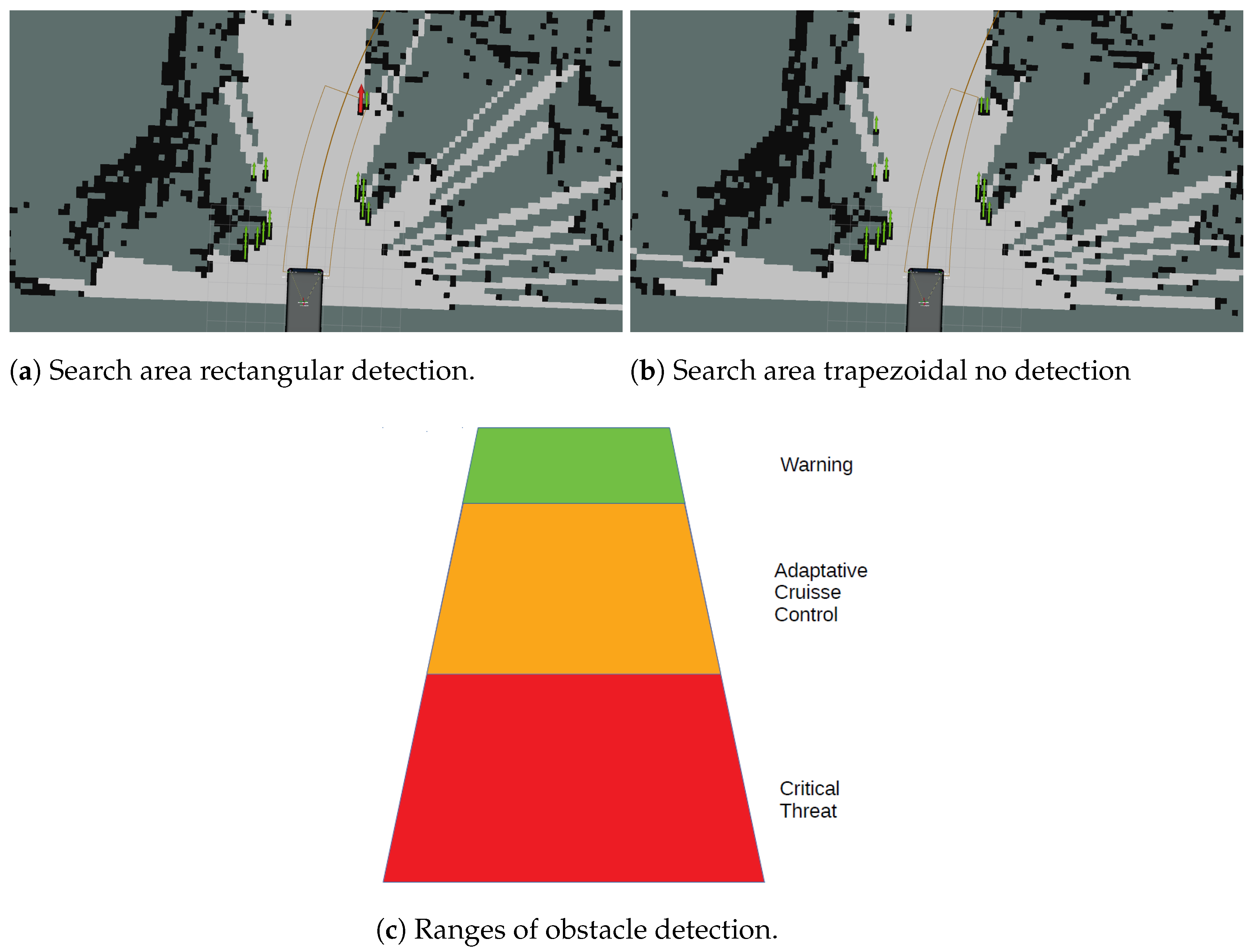
One of the requirements for the research platform as a possible application in tourism areas, airports or similar places is the possibility to work with people around it or with dynamic obstacles. For this reason, the system must implement a methodology that needs to be able to detect and manage obstacles and to decide in the future which set of actions must be performed: avoid the obstacle, regulate the speed, stop the platform in a critical situation, etc. In addition, when dealing with non-standard environments, the narrow path of the rough terrains during the experiments has proven the issue of using naive implementation for detecting obstacles such as using the straight distance to the nearest obstacle in the route.
Thus, the solution proposed in this work is to search within a boundary area based on the predicted trajectory the vehicle decided to follow; this trajectory is computed online with the speed and steering angle reported from the low level of the vehicle. Hence, the boundary area is computed from this predicted path and it is updated dynamically in longitude and aperture, changing its shape depending on the vehicle speed to detect further distances and to react in time for any possible obstacles that lie inside the trajectory. As a result, the area can be wider and/or higher depending on the predicted trajectory and/or be narrower the farther away it is from the platform. This setup allows the system to avoid false positives in narrow corridors and rough environments for the final shape is a trapezoidal area and can be tuned with more precision than a rectangular one.
Due to this, the area is divided into dynamic regions where the proportions are constant and the longitude is determined by the speed of the platform. For instance, the maximum speed established for the vehicle is 4 m/s and the maximum search trapezoidal area is 10 m. Since the area is divided into several sections, there are several decision-making processes to perform at each one. For the green zone in
Figure 14c that comprises between 100% to 90% of the area, any obstacle is detected but with no repercussion in the control and it only has to be ready for action; for the orange section that lies more or less in the middle of the area, the vehicle reduces the speed proportionally to the distance of the object detected and this means that, for the range between 90% and 50%, the vehicle regulates the speed based on obstacle distance; and, finally, for the last area below to 50%, which is the one in red, the vehicle stops since it is a critical section, which can be defined by a threshold distance of 3 or 4 m for instance.
3.6. Control
3.6.1. Model Predictive Controller (MPC)
For the control based on odometry for this platform, the approach of the MPC has been used to ensure a robust generation of control commands. The MPC is now widely accepted for the lateral control such as [
15,
16] and has been used in several platforms for autonomous vehicles, one of them seen in [
17]. Due to the stability and convergence of control commands, this method has been selected over the Stanley method [
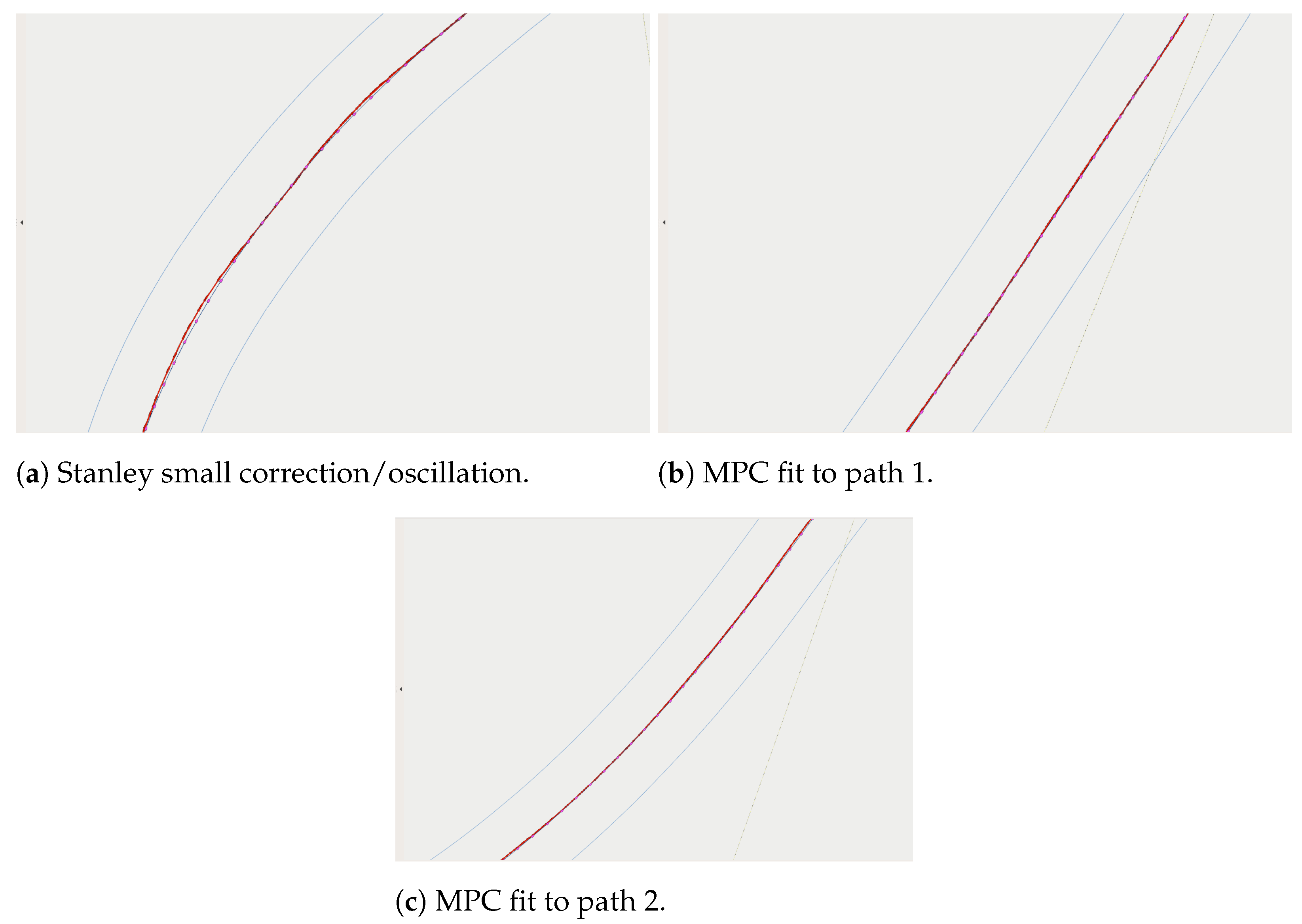
18] proposed in the DARPA Grand Challenge. Both solutions were proved valid for low speed as a control method for the vehicle selected, however, the MPC provides better results for this vehicle in sharp curves and a closer path following as shown in
Figure 15. It is possible to observe the performance of a little corrections in the Stanley method but no oscillations in the MPC method.
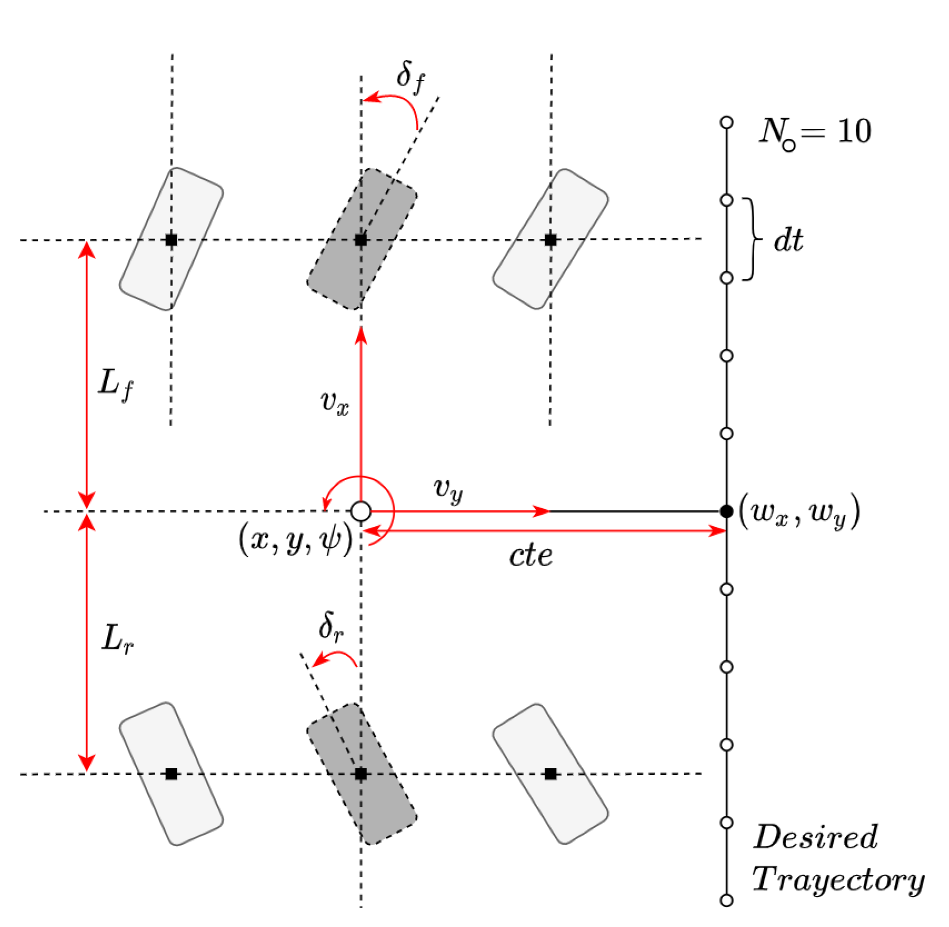
As a brief introduction to the MPC, it must be said that is a method of control usually used to govern a system while satisfying a set of arbitrary constraints defined. In this particular case, the system that is to be controlled is the lateral and longitudinal behaviour of the platform. The task is to follow a trajectory and this is defined in the MPC as an optimisation problem to generate the most suitable trajectory to follow by simulating different actuators inputs in several time steps. In Equation (
11) the plant model is depicted in which it is defined how the vehicle is modeled within the controller. Moreover, in
Figure 16 it is shown how the vehicle state is defined geometrically. In this model
is the vehicle local position,
the orientation,
v the speed,
the cross-track error and
the orientation error with respect to the path. The MPC uses
N steps in the future divided in
times fractions to simulate a set of trajectories, taking into account Equation (
12) constraints and extracting the most suitable one from a cost function defined in Equation (
13). This function penalizes the vehicle state depending on the configuration provided with the weights (
w) that allows the adjustment of the controller to fit new vehicle models or give more importance to certain variables.
Hence, with this approach the vehicle is able to follow the pre-computed path with almost no deviation.
3.6.2. Road Reactive Control
The second and backup method for control is the Road Reactive Control (RRC) that uses the information provided by the road detection module in conjunction with a PID controller Equation (
14) checking the distance from both boundaries (
and
) where the error
e Equation (
15) is the distance difference from the centre of the road. However, it must be said that the road in the whole trajectory is mostly constant with some exceptions such as intersections or road openings. The Road Reactive Control takes as input the yaw estimation with respect to the road boundary limits computed with the 2D road model within the Road detection module. This provides a representation on how the vehicle drifted away from the middle of the road. In the case that the platform is deviating from the middle, the PID controller produces the necessary steering commands that will likely make the platform stay in the middle of the road. This corrections perform cyclically each time and the Road detection module produces new road/vehicle state information.
Moreover, to avoid the problem of the road openings and intersections, the odometry and path manager modules are in charge of detecting several points in the route to activate the mode of path decision in intersections, switching the controller from the RRC to the odometry control based on DGPS and UKF for this section and changing it back when necessary.
3.6.3. Speed Manager
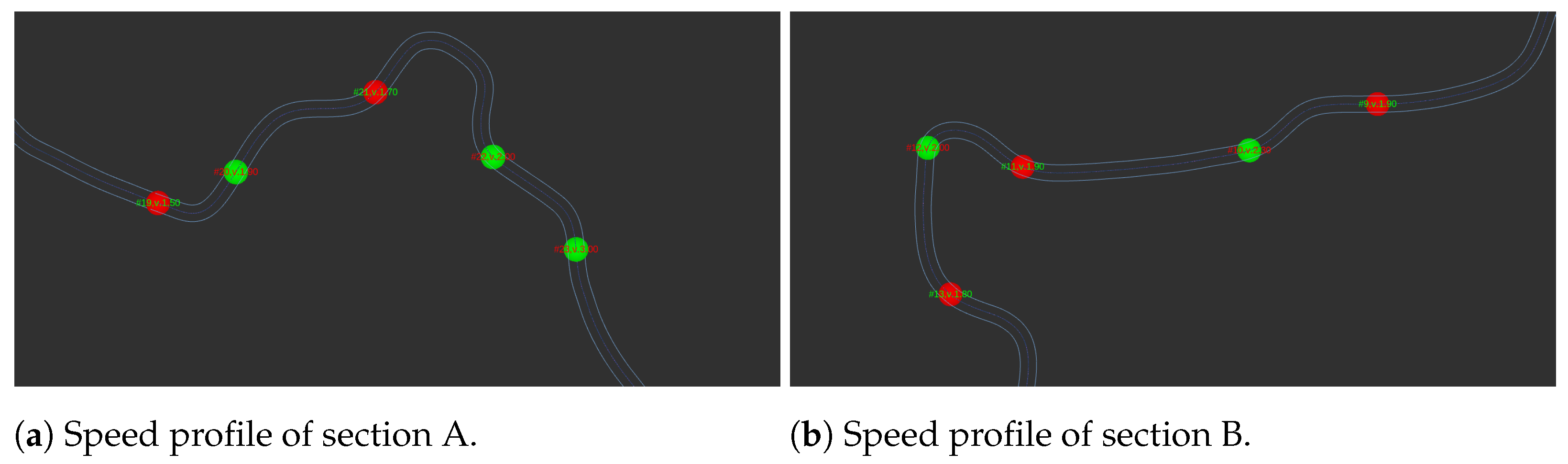
Since the pre-computed path is composed of a huge set of waypoints and since it is necessary to decide which speed limits must be given to the platform in each path section, there must be a process in which a speed profile is computed for the whole path. Thus, the generation of this speed profile is performed automatically based on the geometry of the road and the maximum desired speed of the vehicle in turns. Furthermore, the calculation aims to enhance road holding and passengers comfort. In this manner, the road curvature is analyzed, which can be obtained easily once knowing the path, and by using the normal curvature radius formula.
By analyzing the curvature profile, straight sections on the road are identified as those with curvature radius that approach infinity, whereas the curvature radius in turns can present very different values that can be close to 0 in extreme cases. The first approach is to define the speed in straight sections as the maximum desirable speed and to define a variable speed in turns depending on their curvature radius. After this and for safety reasons, the speed is reduced in the proximity of turns. To reduce the size of the speed profile to only the relevant indexes of the path where the speed must change, filtering is performed so that the path is reduced to single-speed sections.
Figure 17 shows a two-path section processed to generate the speed profile. Each section the path is presented as a finite set of poses and the speed assigned to each sector as green circles (if it is an acceleration sector) or red circles (if it is a deceleration sector), the
# means the speed sector number used to track and test the profile.
3.6.4. Control Manager
The Control Manager is the module in charge of determining which method of control the platform is going to use for its high-level control interface. It takes all the control commands the control modules generates and some sensor information and decides which control method to trust.
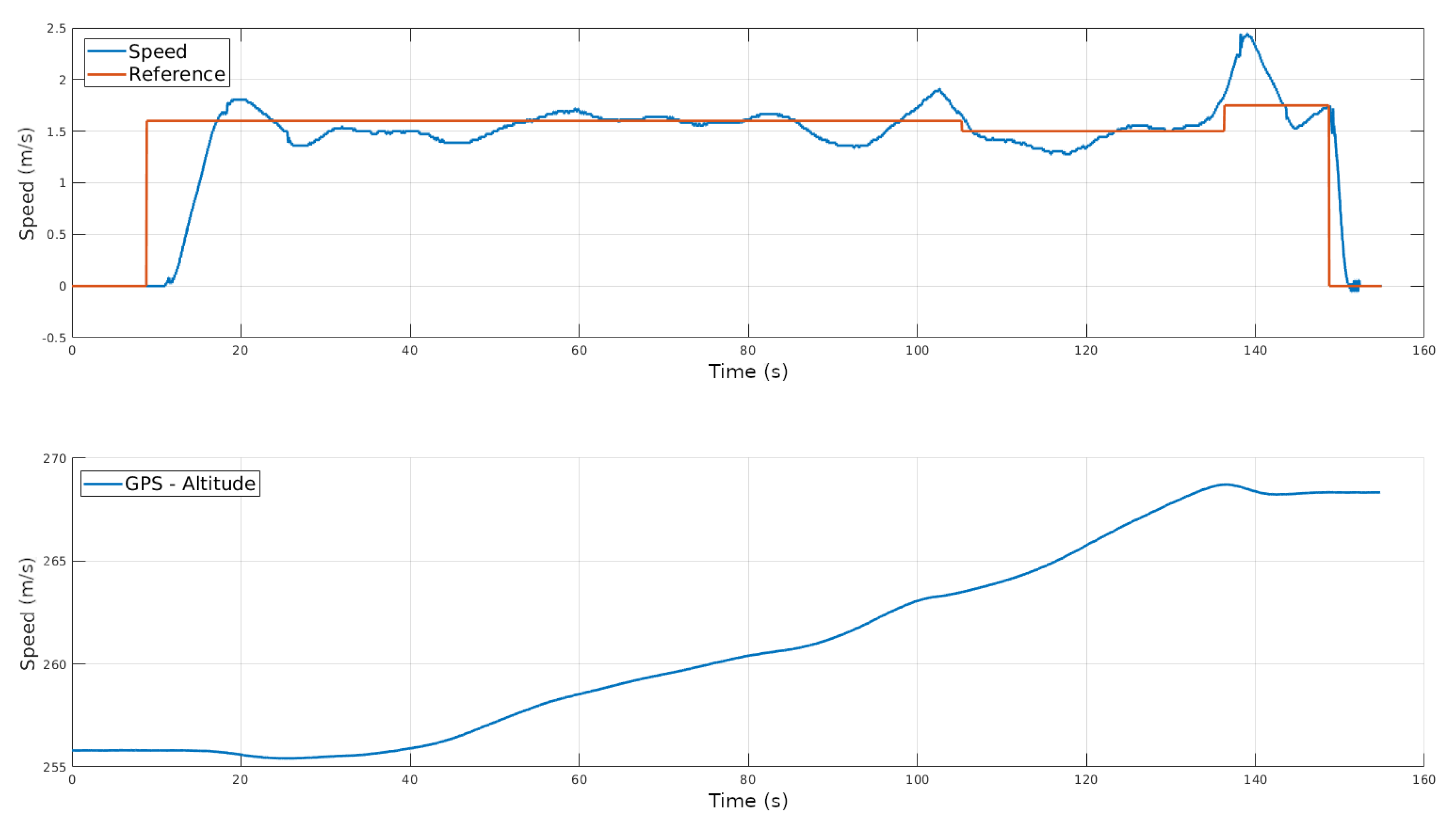
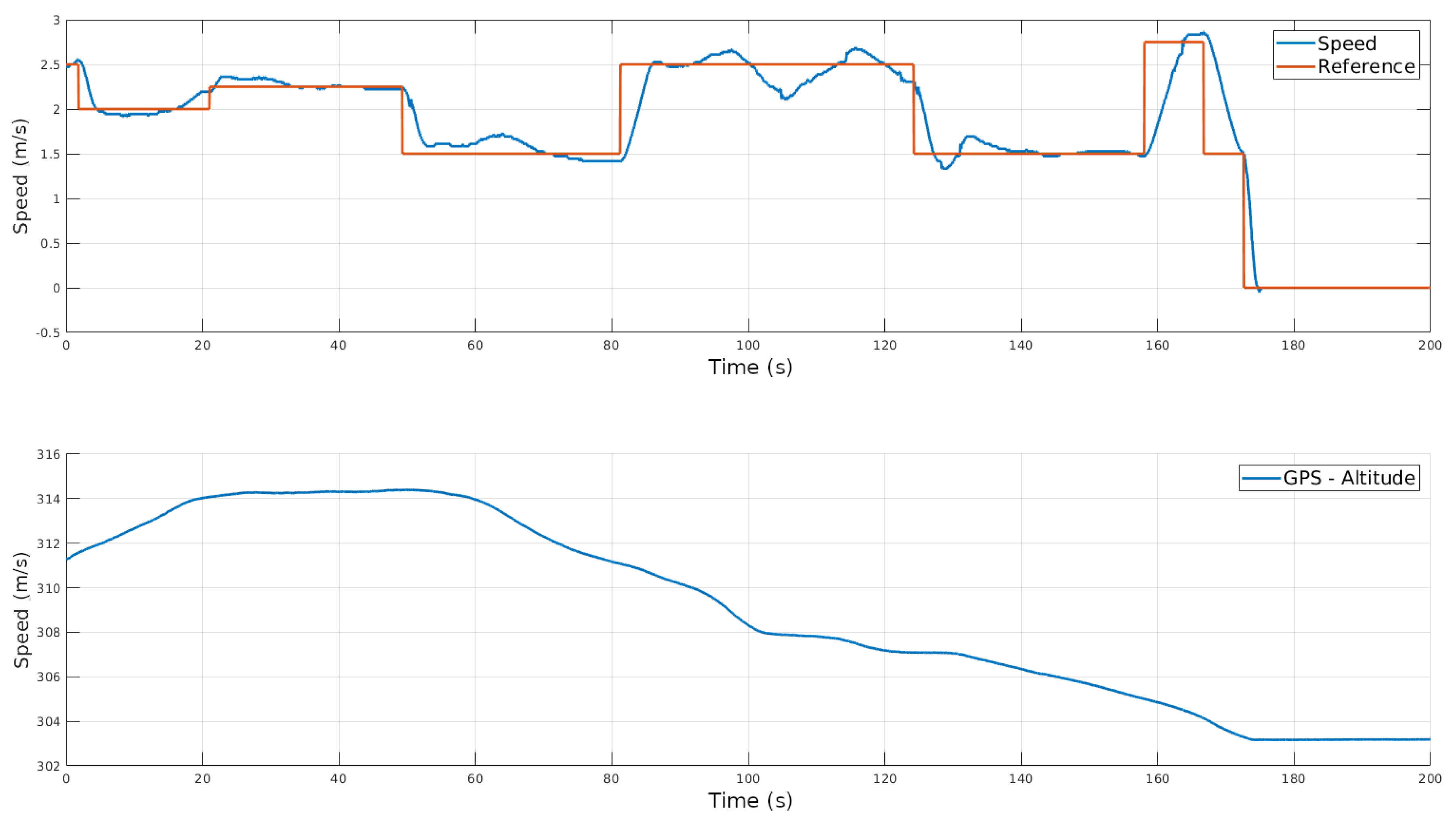
As previously specified, the low-level control of the vehicle is the original control from the EZ10 LIGIER model. On one hand, the speed reference, acceleration and steering angle are generated from high-level modules and the vehicle can follow the reference as
Figure 18 for uphill and
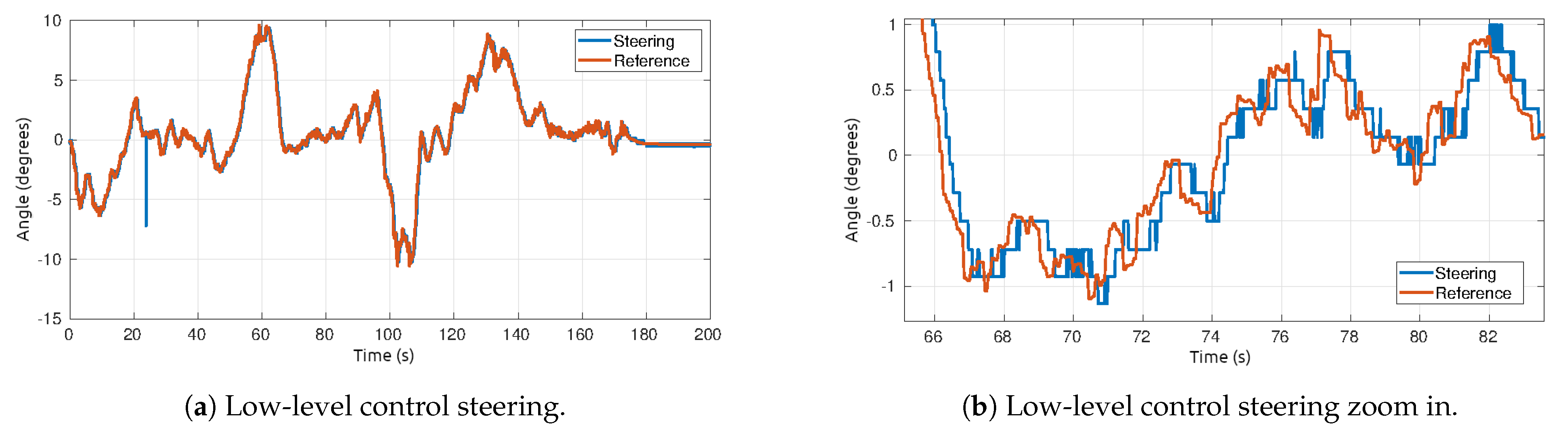
Figure 19 downhill where it shows the reference velocity generated from the high-level control and the current speed. Additionally,
Figure 20a shows the steering angle commands generated from the lateral control and the current steering angle where
Figure 20b is a zoom-in of the same figure. It is possible to appreciate the following action of the steering wheel. Depending on the slopes, accelerations and speed configuration, the vehicle is able to follow as commanded with no additional control steps performed by the team. On the other hand, the system implements two nodes generating control commands for the platform to follow the path. One is based on localization and path planning, which is the Model predictive controller (MPC), and the second one is based on road detection and both methods were described in the former sections. However, the important part here is how the vehicle decides which control method to trust and that is performed by considering the score computed in
Section 3.1.2 that is in charge of processing sensor data, allowing the platform to switch between the controllers used in this particular instance of the software architecture. The primary option, if the score is higher than a threshold, is the MPC method due to its robust performance. However, if the localization score computed from odometry is not high enough, the control manager will not trust any command sent by the MPC and the reactive road controller will provide the commands for the vehicle. This method was proved sufficient to computed in practice where the threshold limits must be placed in order to manage the control inputs. Furthermore, there is a more important fact here to bear in mind and it is related to how the covariance estimations of the Odometry and Road detection modules are computed, which that goes out of the scope of this work. While other solutions may want to complicate this problem unnecessarily, this particular approach turned out to be sufficient in order to ensure good navigation with unnoticeable recovery behaviours. Although it must be stated that once the system proposed is enhanced with new control and localization methods, it would be advisable to improve this selection method with more suitable approaches.
3.7. Self Awareness
Once the system can navigate and fulfill the project requirements, it is necessary to have the certainty of a healthy and working system. To do so and to provide a high degree of security and robust functioning, two modules have been developed to maintain the running of the whole system without any incompatibility or risk. In this manner, there are two levels of risk: in level one, which is a critical risk, it will be necessary to stop the vehicle immediately as in an emergency stop and will require human intervention to rearm the platform. In the second level, which is a low risk, the vehicle will reduce the speed slowly and stops until the anomaly is solved; once is solved it will be able to continue on the route automatically.
3.7.1. Sensor Awareness
To complete this task, the first module is the sensor awareness in which the data produced by the sensors is analyzed to know if the sensor is running and working properly. This module checks the frequency of the message for each sensor published and the content of its data. On one hand, for each LiDAR, the frequency is 10 Hz and the data gathered should be at least the minimum set of points that hits the road. To count the points, several experiments have been carried out in which each sensor is covered by an opaque blockage. Because the LiDAR Point Cloud in the nearby space is filtered as described in
Section 3.5.1, the data flow upstream in the architecture will receive zero points. The sensor awareness detects this anomaly and sends the proper flag to the movement manager to stop the vehicle immediately since a level one anomaly is happening. On the other hand, the IMU awareness checks the rate is over 30 Hz and its data are not the same in a time taking into account the sensitivity of the sensor is high. Furthermore, the DGPS awareness is based on the rate (bigger than 4 Hz) and the information provided of the covariance provided with its message that should be at least, with a certain time, accurate enough (that is lower than a threshold). Due to some DGPS coverage lost in some sections of the experimentation environment, the time threshold calculated in which no DGPS signal is received is no longer than 5 min. In the case that this is not fulfilled, the Sensor awareness will be sent the stop signal to mark a level two critical risk.
3.7.2. Software Awareness
The second module that checks how the system is performing and if all its modules are alive and working then it is a node that pings every half second and all ROS nodes that are included are on a specific white list. If for some reason, one of these modules is down, the software awareness sends a level two signal to stop the vehicle because of a low-level risk. Furthermore, for every ROS node, there is a respawn procedure that allows the platform to restore each module that is somehow killed or shut down. Moreover, as a final remark, the only nodes that can stop the vehicle with an emergency stop (level one awareness) is the movement manager and the low-level control bridge for security reasons.
3.8. Cybersecurity
This section lists the main potential cybersecurity risks that can occur during autonomous vehicle service. In addition, the technical measures used to establish solutions to these risks and minimize their impact will be established.
3.8.1. Communications Architecture
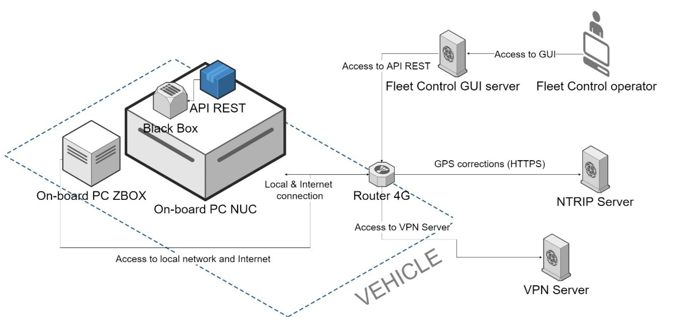
The different hardware and software components that make up the information system and communications architecture of the autonomous vehicle are listed in
Figure 21.
The components of the vehicle communication architecture can be grouped as follows:
On-board communications equipment and infrastructure. In this group, we have the following elements.
- –
NUC onboard PC, where most of the control software nodes, the black box and the REST API that serve information to other systems run;
- –
ZBOX on-board PC, where the heaviest computational-level sensor information processing nodes run;
- –
The 4G router. The equipment mentioned above is connected to a router by a local gigabit ethernet network and the Internet by 4G connectivity through this same device. Requests made to services that run on vehicle computers will arrive through this infrastructure.
Equipment and infrastructure outside the vehicle. These are all the information systems that obtain data from the vehicle but which physically reside outside of it and therefore its local network.
- –
NTRIP server. The vehicle’s control system makes requests to this server to obtain differential corrections that improve the precision of the vehicle’s location;
- –
Fleet control GUI server. Provides the fleet control GUI service that allows checking the correct performance of the vehicles in the fleet and geolocating them on the map. In addition, this service makes requests to the REST API of the vehicle to obtain its status information;
- –
VPN server. It provides the service that supports the virtual private network to which both the onboard equipment and the server where the fleet control GUI is hosted are connected.
3.8.2. Computers in Virtual Private Network
It is important to note that the equipment external to the vehicle, which needs to be connected to the equipment on board to obtain information, will do so through a Virtual Private Network (VPN). The VPN provides an encrypted communication channel between the equipment inside of this network and prevents a computer that is not authorized within the VPN from being able to access any computer that is inside and, consequently, if a computer external to the bus is not connected to the VPN, it will not be able to access the equipment on board. The virtual private network service is hosted on a server external to the vehicle and managed and guarded by the autonomous vehicle development team. The necessary credentials will be provided to those authorized servers external to the minibus that need to access the services running on the on-board computers
3.8.3. Security Mechanisms Implemented to Prevent Cyber Attacks on Information Systems
The technical measures carried out to deal with cybersecurity threats are listed below concerning the vehicle’s internal and external communication systems.
Threats to computers installed on board. A permission policy is established on the files and processes of the operating system of the onboard computers so that only the accredited user will be able to interact with the different software elements of the onboard computers. To limit access to the onboard computers from the internet, policies have been established for the router firewall and the operating system firewall of the onboard computers. In case of attempted physical access to the vehicle, access for users with administration permissions is protected by two-factor access credentials. Policies have been implemented to recover services in case of a shutdown. The hard drives installed in the onboard computers are encrypted so that the information and source code cannot be accessed in case of physical theft of the equipment. The only service accessible by computers from outside the vehicle is the REST API. This service is only accessible through the VPN, making use of the HTTPS protocol through port 443, which the only accessible port of the onboard computers and avoids the violation of other services such as the vehicle control system. To access the REST API service, the client must authenticate with valid credentials. Once accepted, They will be granted an access token for a limited time, which they will have to renew once it has expired. All the services that make up the black box system run in isolation from the native operating systemby using containers.
Threats to servers outside the vehicle. A permission policy is established on the files and processes of the operating system of the onboard computers so that only the accredited user will be able to interact with the different software elements of the onboard computers. To limit access to these servers from the Internet, a firewall policy is established that only allows access through the port exposed by the service used. The services run in isolation from the native operating system by using containers. Communication with the services is encrypted by using the HTTPS protocol. Physical access to external computers is not allowed. The services provided by external servers do not provide methods to control the vehicle remotely or allow the data stored in it to be altered. A policy is established to limit the consumption of resources on each of the containers that host the services. Policies have been implemented to recover external services in case of their stoppage.
Threats regarding the communication channels between vehicle and servers. Communications between vehicle and servers are encrypted using the HTTPS protocol. Moreover, additional encryption is established between the onboard and external computers through the VPN. The nature of the services displayed in the vehicle does not allow interaction with the vehicle’s control system in case of impersonation. The attributes of the messages received in the vehicle are verified and validated in the REST API Service. If the REST API service detects an abnormal flow of requests from a specific IP and it will ignore the requests received from that source, entering a blacklist of untrusted sources and notifying those responsible. WAF and IDS systems are used for the detection and prevention of denial of service attacks.
Threats to vehicles regarding their upgrade procedures. A user permission policy is established where updates can only be made with authorized credentials. A security policy is established on updates to control software and drivers, with which the version of these is verified and the vehicle is prevented from starting in case of detecting any anomaly.
Penetration tests. Penetration tests have been carried out to determine the degree of access that an attacker with malicious intentions would have, identify the vulnerabilities to which said assets are exposed and establish action plans to mitigate the potential effects caused by the threats detected.
3.9. User Interfaces
For this autonomous vehicle, several software components have been established that allow human interaction with the vehicle through Graphical User Interfaces (GUI). The following have been implemented:
Operator interface. It allows the person in charge of managing the vehicle on the road to view the vehicle’s status parameters and interact with it by performing some basic actions such as starting a route, pausing and opening doors or ramps among others;
Black box interface. Allows auditors to query and export vehicle health records stored in the black box system in the last 7 days;
Fleet interface. It allows the person in charge of controlling the autonomous vehicle fleet to be informed in real-time of their location and any relevant event that may arise on the route. It will also inform if a vehicle is delayed in completing the itinerary from one point of interest to another.
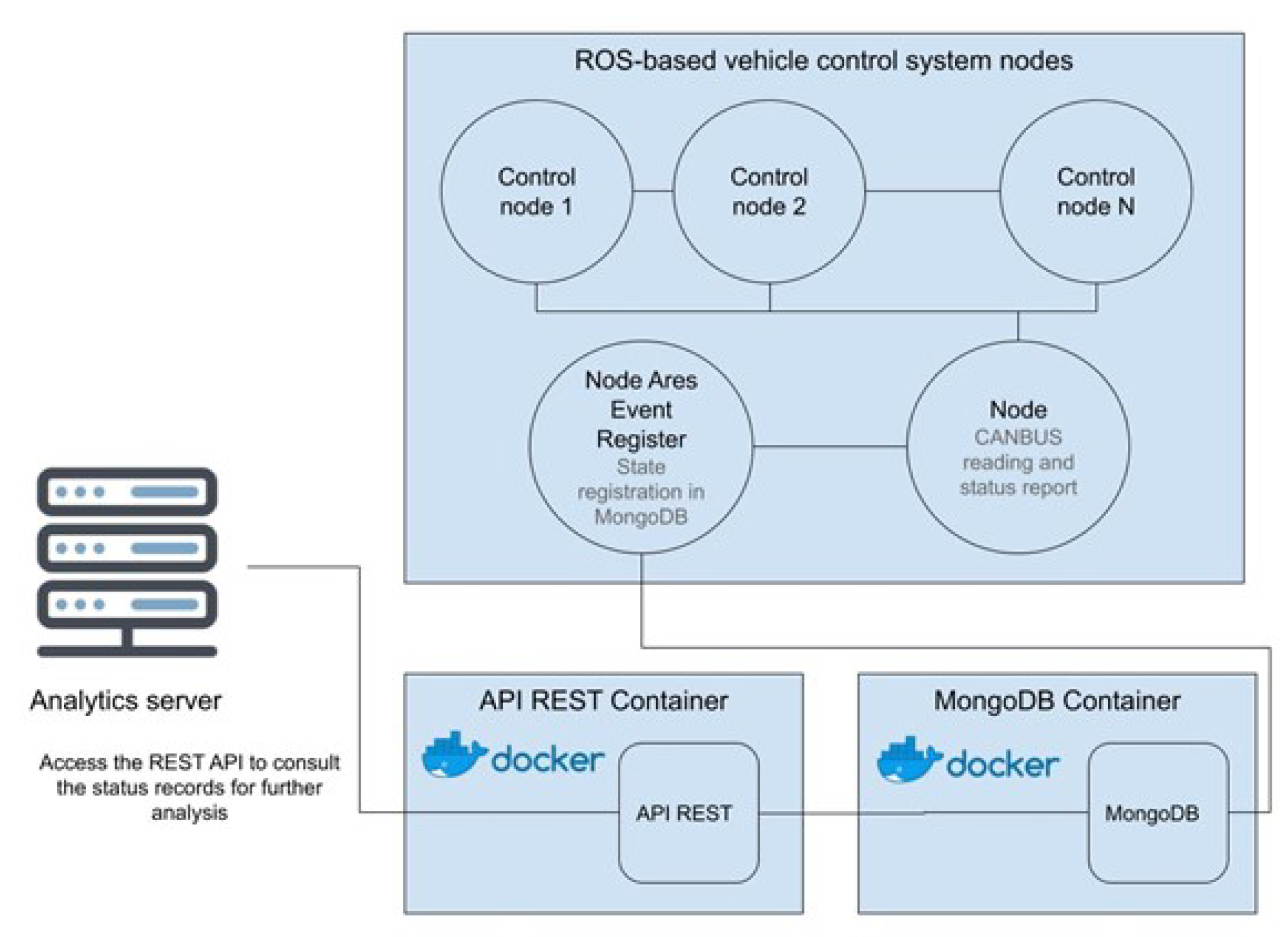
3.10. Black Box System
In addition, a black box system has been implemented that allows the recording of relevant information on the vehicle’s status such as its location, speed, steering or sensor status. This black box system consists of three components:
Permanent Storage System. Stores a complete record of the vehicle’s status every second. This record is in JSON format and is stored in the MongoDB database management system;
Ares Event Register. ROS node that receives the relevant information from the vehicle control system through ROS and stores it in the Permanent Storage System;
Ares API REST. Allows queries about the records stored in the Permanent Storage System.
In the diagram in
Figure 22, you can understand how these three subsystems communicate with the vehicle’s control system. The REST API and MongoDB components have been packaged in containers using Docker technology. This allows them to be run in isolated environments, with the consequent improvement in their handling and safety.


 ,
, 


