
Optimization-Based Antenna Miniaturization Using Adaptively Adjusted Penalty Factors


Abstract
:1. Introduction
2. Optimization-Based Antenna Miniaturization
2.1. Problem Formulation
2.2. Trust-Region Gradient-Based Algorithm
3. Size Reduction with Adaptive Penalty Coefficients
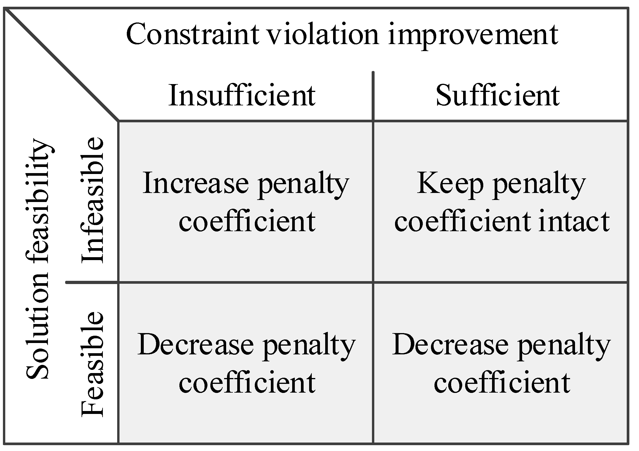
3.1. Adaptively Adjusted Penalty Factors. The Concept
- If the parameter vector x(i+1) produced at the iteration i is feasible from the point of view of the jth constraint, the corresponding penalty coefficient βj may be reduced;
- If x(i+1) is infeasible but the violation of the jth constraint was reduced to a sufficient extent w.r.t. the (i–1)th iteration, the coefficient βj remains intact;
- If x(i+1) is infeasible and there was no improvement of the jth constraint violation or the improvement was insufficient, the coefficient βj should be increased.
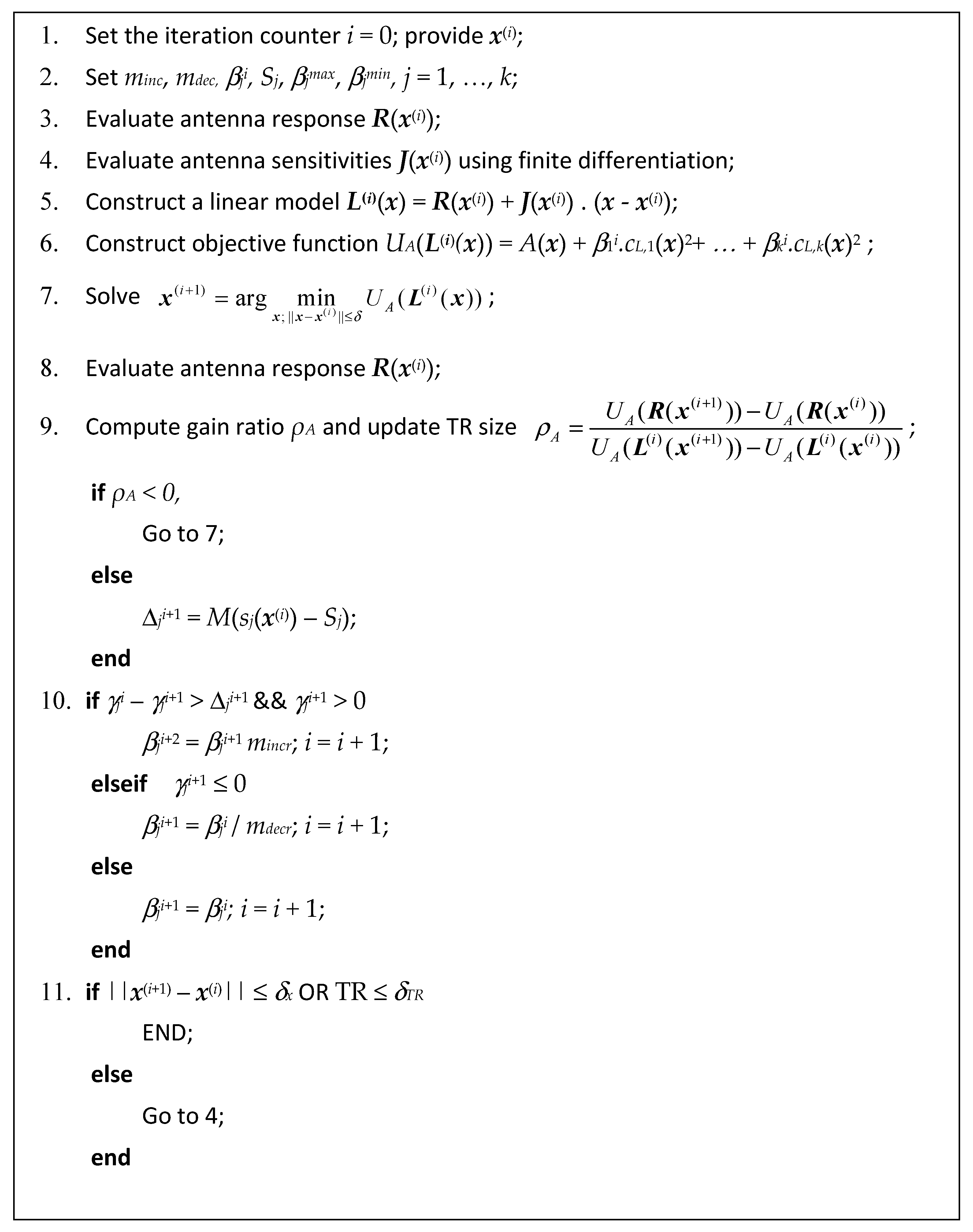
3.2. Adaptively Adjusted Penalty Factors. The Procedure
| if γji+1 ≤ 0 |
| βji+1 = βji/mdecr; |
| else |
| if γji − γji+1 > Δji+1 |
| βji+1 = βji; |
| else |
| βji+1 = βjimincr; |
| end |
| end |
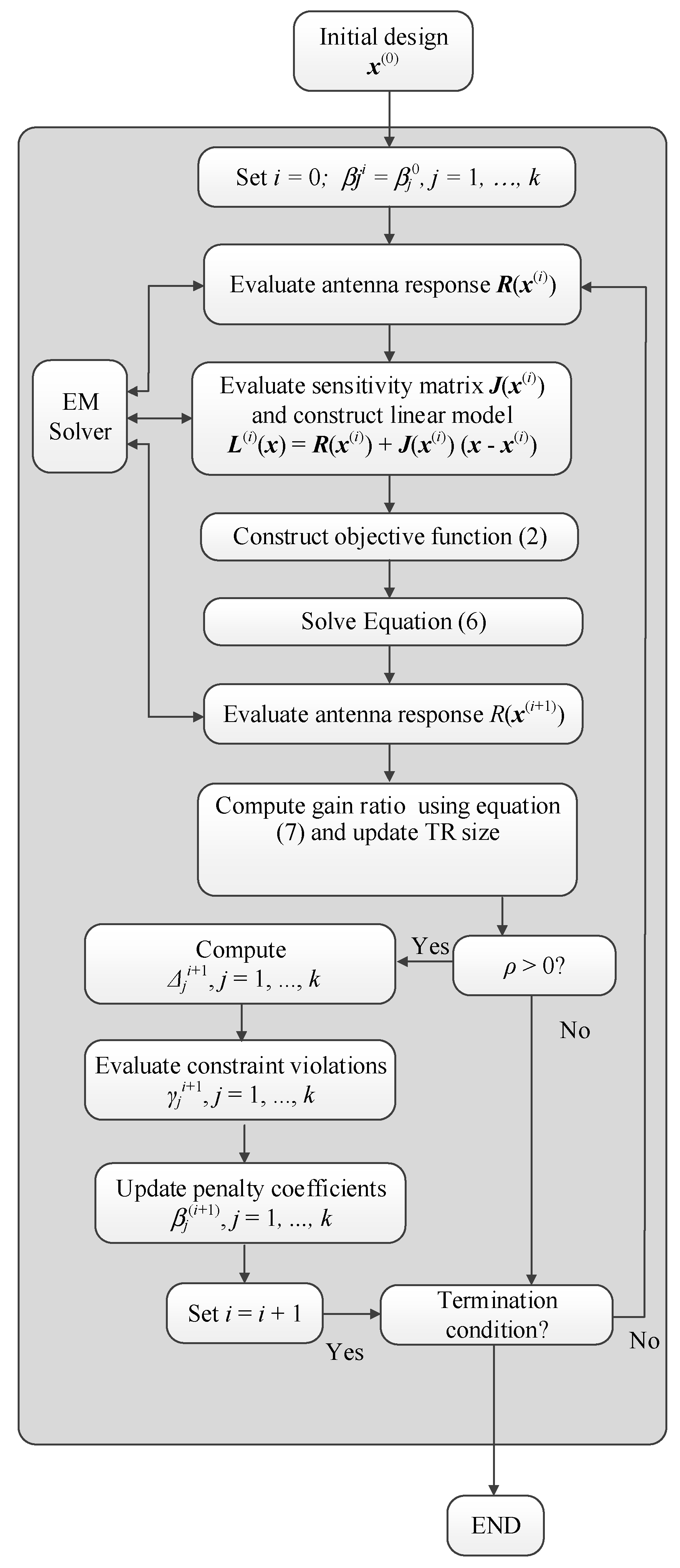
3.3. Optimization Framework
- minc, mdec—increase and decrease factors for the automated adjustment of penalty coefficients (cf. Section 3.2);
- M—a factor used to determine sufficient constraint violation improvement (cf. Section 3.2);
- βjmax, βjmin—maximum and minimum values of penalty coefficients; j = 1, …, k;
- βj0—initial values of the penalty coefficients; j = 1, …, k;
4. Verification Case Studies
4.1. Experimental Setup
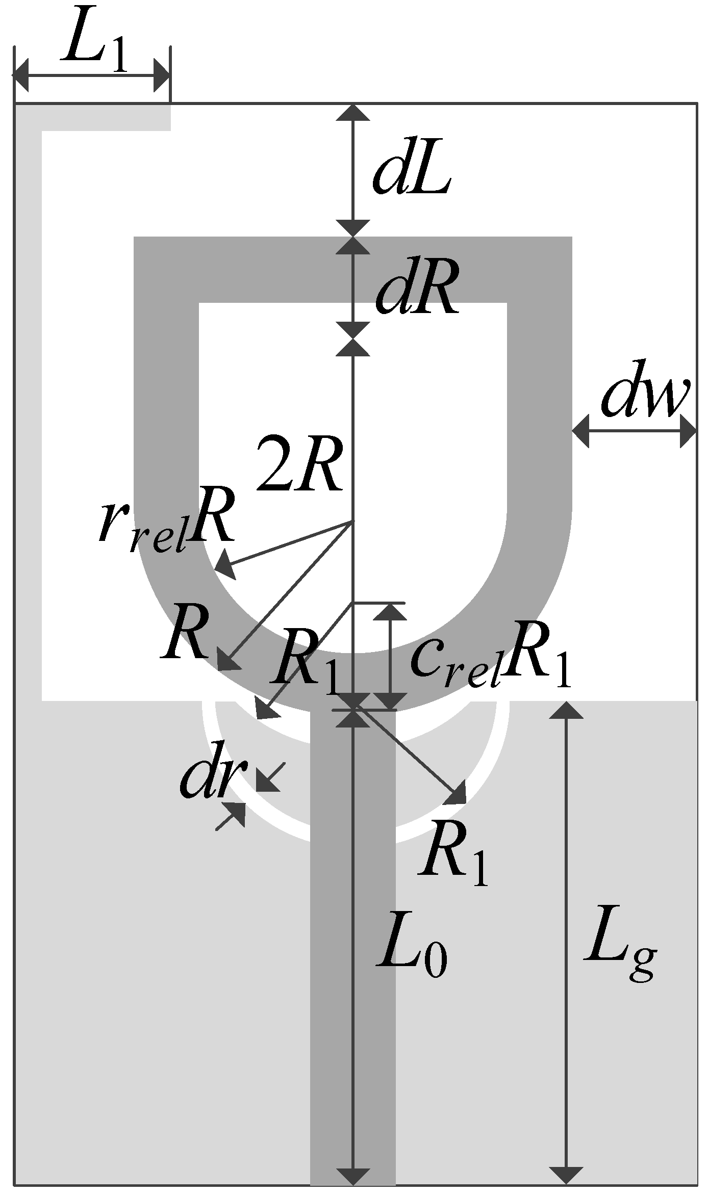
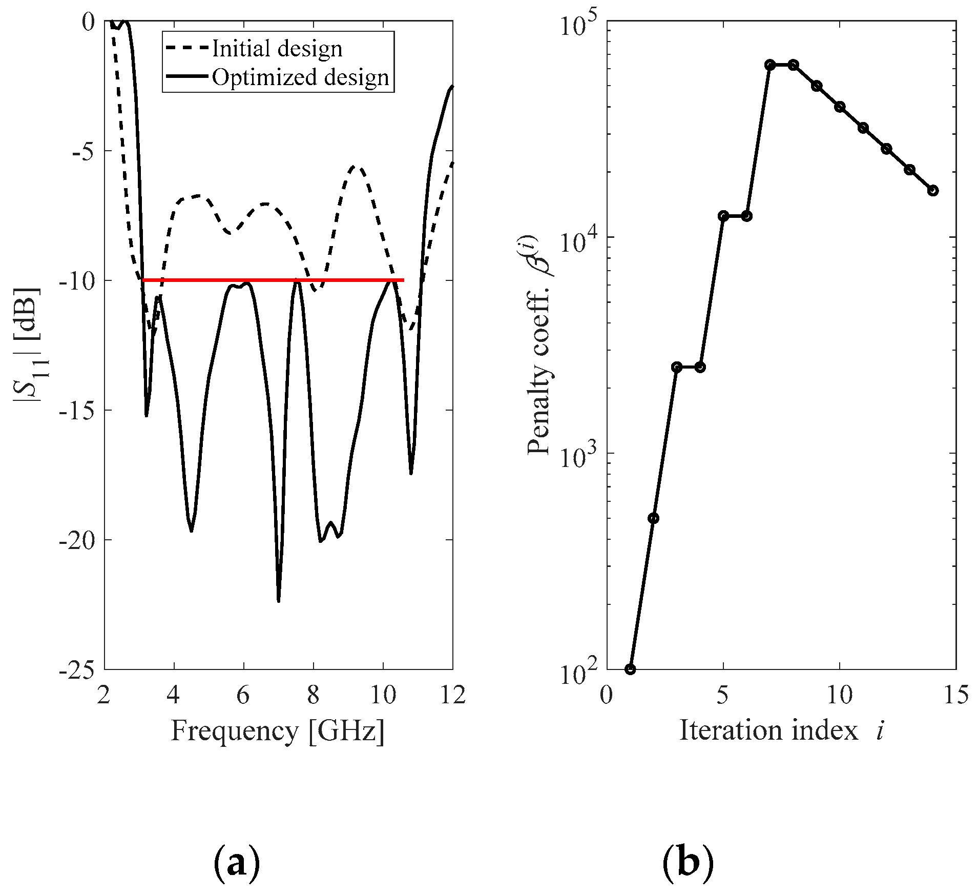
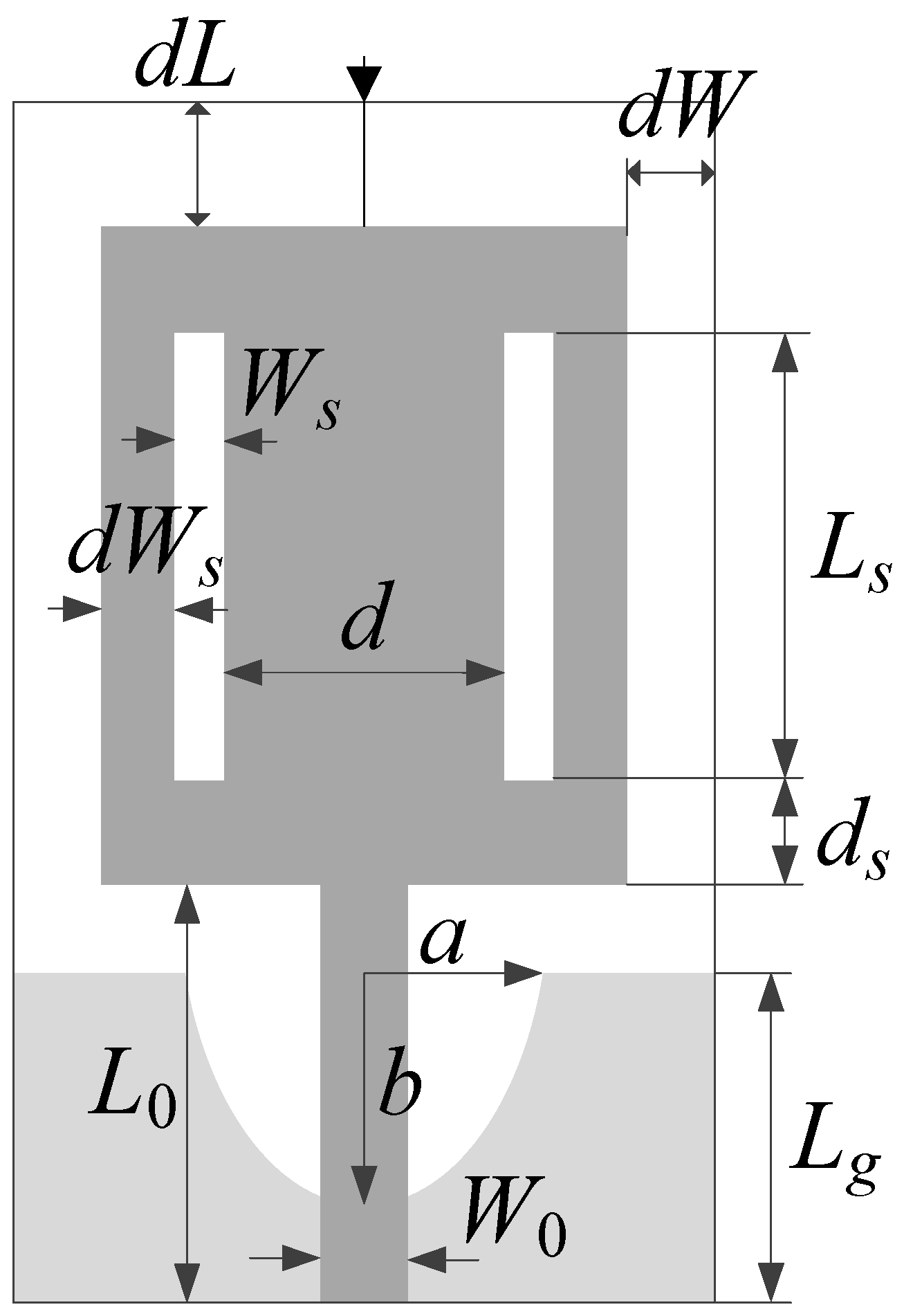
4.2. Antenna I
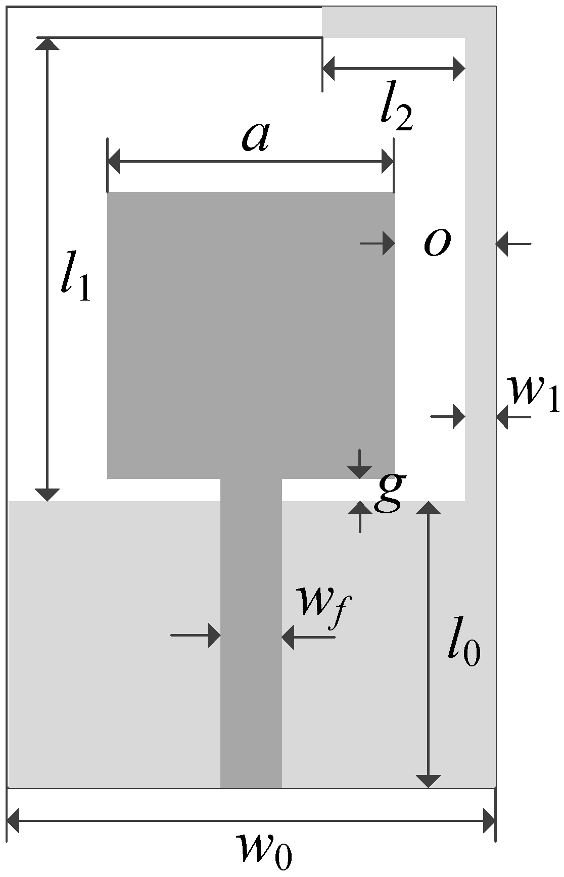
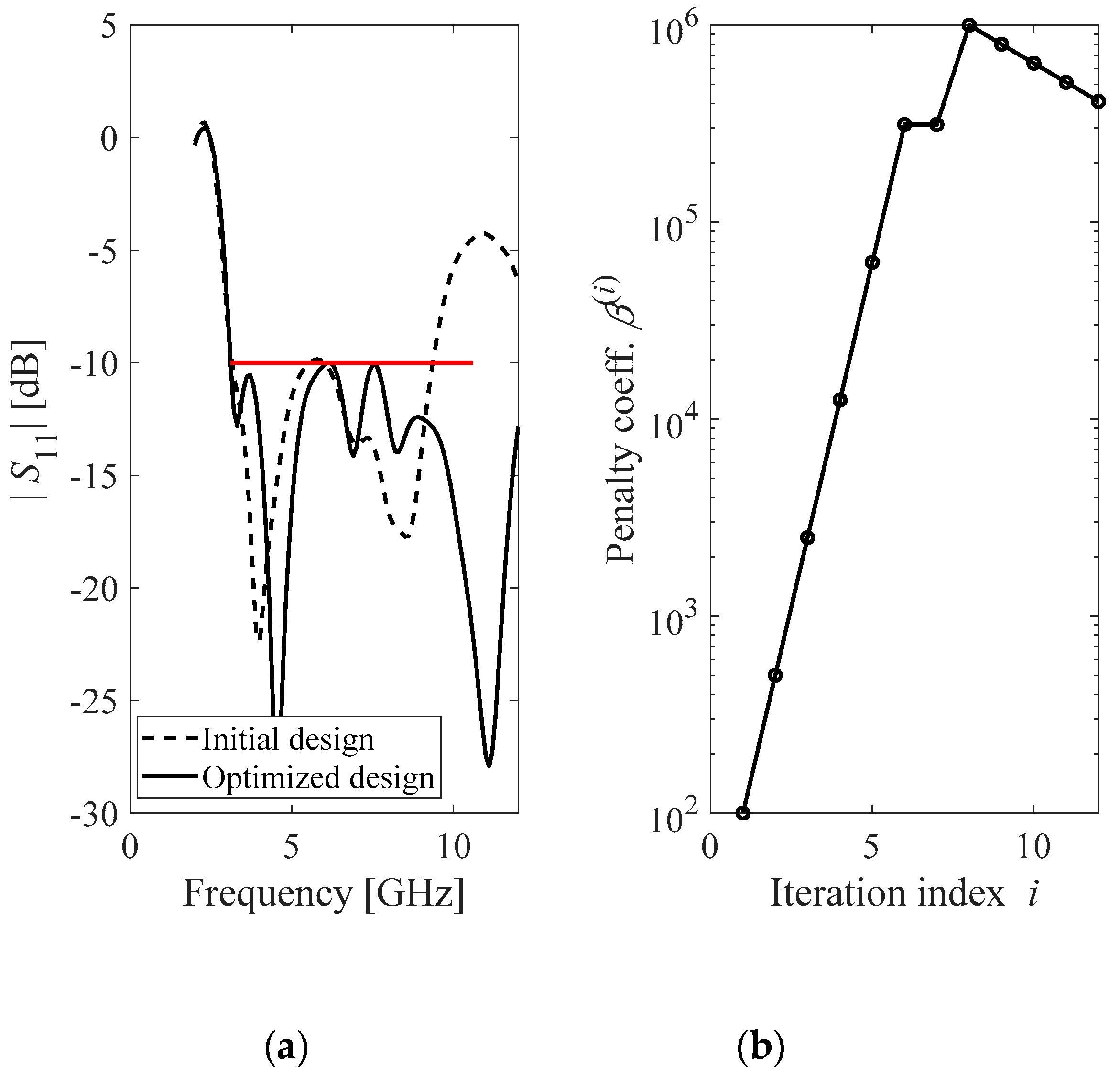
4.3. Antenna II
4.4. Antenna III
4.5. Discussion
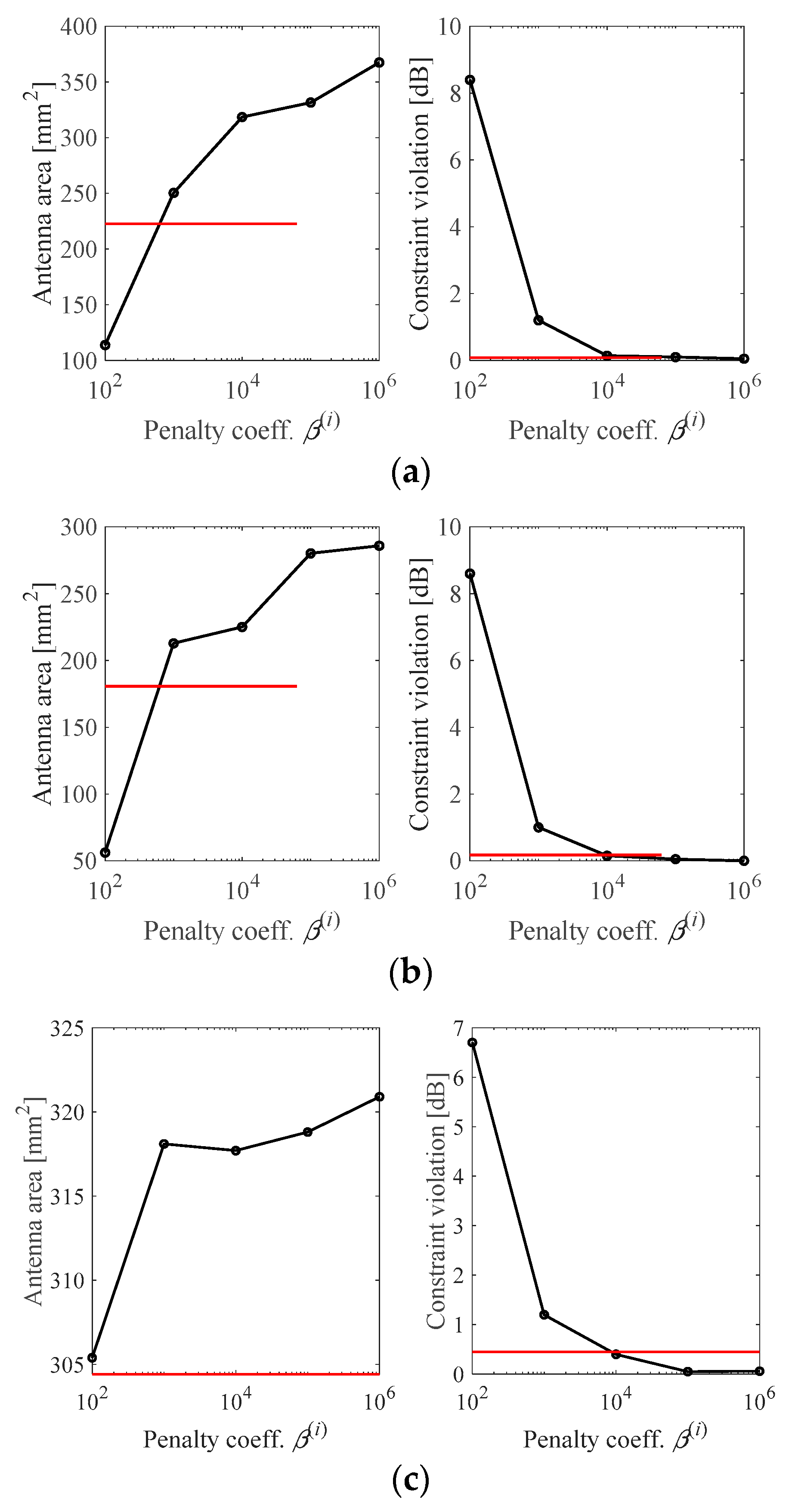
- Although the optimum value of penalty coefficient in the fixed-setup optimization seems to be about β = 104 for Antenna I, between β = 103 and β = 104 for Antenna II, and between β = 104 and β = 105 for Antenna III, considering the achievable miniaturization rates along with sufficient constraint satisfaction, the optimum value of penalty coefficient is problem-dependent. The optimum values should be identified for particular iterations of the optimization process and they are generally dependent on the status of constraint violation.
- In both fixed and automated adjustment setups, using a penalty coefficient lower than the optimum value, results in significant constraint violation. As for the former, the violation can easily become as high as five times of the tolerance threshold or even more. Antennas I and II are representative examples of this design quality degradation.
- Automated adjustment of penalty coefficients seeks to improve the final design quality by the optimum value of penalty coefficients at the level of iterations of the optimization process. This, in turn, permits a better control of constraint violations along with better achievable miniaturization rates.
- The performance improvements are significant. For the corresponding levels of constraint violations, the procedure proposed in this work leads to antenna footprints that are smaller by 110, 44, and 13 mm2 for Antenna I, II, and III, respectively.
5. Conclusions
Author Contributions
Funding
Acknowledgments
Conflicts of Interest
References
- Le, T.T.; Yun, T.-Y. Miniaturization of a dual band wearable antenna for dual-band WBAN applications. IEEE Antennas Wirel. Propag. Lett. 2020, 19, 1452–1456. [Google Scholar] [CrossRef]
- Agneessens, S.; Rogier, H. Compact half diamond dual-band textile HMSIW on-body antenna. IEEE Trans. Antennas Propag. 2014, 62, 2374–2381. [Google Scholar] [CrossRef] [Green Version]
- Upadhyay, D.; Dwivedi, R.P. Antenna miniaturization techniques for wireless applications. In Proceedings of the 2014 Eleventh International Conference on Wireless and Optical Communication Networks (WOCN), Vijayawada, India, 11–13 September 2014; pp. 1–4. [Google Scholar]
- Oraizi, H.; Rezai, B. Dual-banding and miniaturization of planar triangular monopole antenna by inductive and dielectric loadings. IEEE Antennas Wirel. Propag. Lett. 2013, 12, 1594–1597. [Google Scholar] [CrossRef]
- Oh, J.; Sarabandi, K. A topology-based miniaturization of circularly polarized patch antennas. IEEE Trans. Antennas Propag. 2013, 61, 1422–1426. [Google Scholar] [CrossRef]
- Abbosh, A.M. Miniaturized microstrip-fed tapered-slot antenna with altrawideband performance. IEEE Antennas Wirel. Propag. Lett. 2009, 8, 690–692. [Google Scholar] [CrossRef] [Green Version]
- Abbosh, A.M. Miniaturization of planar ultrawideband antenna via corrugation. IEEE Antennas Wirel. Propag. Lett. 2008, 7, 685–688. [Google Scholar] [CrossRef]
- Al-Azza, A.A.; Al-Jodah, A.A. Spider monkey optimization: A novel technique for antenna optimization. IEEE Antennas Wirel. Propag. Lett. 2016, 15, 1016–1019. [Google Scholar] [CrossRef]
- Lalbakhsh, A.; Afzal, M.U.; Esselle, K.P. Multiobjective particle swarm optimization to design a time-delay equalizer metasurface for an electromagnetic band-gap resonator antenna. IEEE Antennas Wirel. Propag. Lett. 2017, 16, 912–915. [Google Scholar] [CrossRef]
- Goudos, S.K.; Siakavara, K.; Samaras, T.; Vafiadis, E.E.; Sahalos, J.N. Self-adaptive differential evolution applied to real-valued antenna and microwave design problems. IEEE Trans. Antennas Propag. 2011, 59, 1286–1298. [Google Scholar] [CrossRef]
- Tomasson, J.A.; Koziel, S.; Pietrenko Dabrowska, A. Quasi-global optimization of antenna structures using principal components and affine subspace-spanned surrogates. IEEE Access 2020, 8, 50078–50084. [Google Scholar] [CrossRef]
- Koziel, S.; Pietrenko Dabrowska, A. Performance-based nested surrogate modeling of antenna input characteristics. IEEE Trans. Antennas Propag. 2019, 67, 2904–2912. [Google Scholar] [CrossRef]
- Song, Y.; Cheng, Q.S.; Koziel, S. Multi-fidelity local surrogate model for computationally efficient microwave component design optimization. Sensors 2019, 19, 3023. [Google Scholar] [CrossRef] [Green Version]
- Director, S.; Rohrer, R. The generalized adjoint network and network sensitivities. IEEE Trans. Circuit Theory 1969, 16, 318–323. [Google Scholar] [CrossRef]
- Paronneau, O. Optimal Shape Design for Elliptic Systems; Springer: Berlin/Heidelberg, Germany, 1982; Volume 3, pp. 42–66. [Google Scholar]
- Jameson, A. Aerodynamic design via control theory. J. Sci. Comput. 1988, 3, 233–260. [Google Scholar] [CrossRef] [Green Version]
- El Sabbagh, M.A.; Bakr, M.H.; Nilolova, N.K. Sensitivity analysis of the scattering parameters of microwave filters using the adjoint network method. Int. J. RF Microw. Comput. Aided Eng. 2006, 16, 569–606. [Google Scholar] [CrossRef]
- Papadimitriou, D.; Giannakoglou, K. Aerodynamic shape optimization using first and second order adjoint and direct approaches. Arch. Comput. Methods Eng. 2008, 15, 447–488. [Google Scholar] [CrossRef]
- Toivann, J.I.; Mäkinen, R.A.E.; Järvenpää, S.; Ylä-Oijala, P.; Rahola, J. Electromagnetic sensitivity analysis and shape optimization using method of moments and automatic differentiation. IEEE Trans. Antennas Propag. 2009, 57, 168–175. [Google Scholar] [CrossRef]
- Koziel, S.; Ogurtsov, S. Model management for cost-efficient surrogate-based optimization of antennas using variable-fidelity electromagnetic simulations. IET Microw. Antennas Propag. 2012, 6, 1643–1650. [Google Scholar] [CrossRef]
- Koziel, S.; Ogurtsov, S. Low-fidelity model considerations for simulation-based optimization of miniaturized wideband antennas. IET Microw. Antennas Propag. 2012, 12, 1613–1619. [Google Scholar] [CrossRef]
- Koziel, S.; Ogurtsov, S. Robust multi-fidelity simulation-driven optimization of microwave structures. In Proceedings of the 2010 IEEE MTT-S International Microwave Symposium, Anaheim, CA, USA, 23–28 May 2010; pp. 201–204. [Google Scholar]
- De Villiers, D.I.L.; Couckuyt, I.; Dhaene, T. Multi-objective optimization of reflector antennas using Kriging and probability of improvement. In Proceedings of the IEEE International Symposium on Antennas and Propagation & USNC/URSI National Radio Science Meeting, San Diego, CA, USA, 9–14 July 2017; pp. 985–986. [Google Scholar]
- Bandler, J.W.; Biernacki, R.M.; Chen, S.H.; Grobelny, P.A.; Hemmers, R.H. Space mapping technique for electromagnetic optimization. IEEE Trans. Microw. Theory Technol. 1994, 42, 2536–2544. [Google Scholar] [CrossRef]
- Ossorio, J.; Melgarejo, J.C.; Boria, V.E.; Guglielmi, M.; Bandler, J.W. On the alignment of low-fidelity and high-fidelity simulation spaces for the design of microwave waveguide filters. IEEE Trans. Microw. Theory Technol. 2018, 66, 5183–5196. [Google Scholar] [CrossRef] [Green Version]
- Bandler, J.W.; Cheng, Q.S.; Georgieva, N.; Ismail, M.A. Implicit space mapping EM-based modeling and design exploiting preassigned parameters. In Proceedings of the 2002 IEEE MTT-S International Microwave Symposium Digest (Cat. No. 02CH37278), Seattle, WA, USA, 2–7 June 2002; Volume 2, pp. 713–716. [Google Scholar]
- Koziel, S.; Ogurtsov, S. Fast surrogate-assisted simulation-driven optimization of add-drop resonators for integrated photonic circuits. IET Microw. Ant. Propag. 2015, 9, 672–675. [Google Scholar] [CrossRef]
- Xiao, L.; Shao, W.; Ding, X.; Wang, B. Dynamic adjustment kernel extreme learning machine for microwave component design. IEEE Trans. Microw. Theory Technol. 2018, 66, 4452–4461. [Google Scholar] [CrossRef]
- Zhang, C.; Zhu, Y.; Cheng, Q.; Fu, H.; Ma, J.; Zhang, Q. Extreme learning machine for the behavioral modeling of RF power amplifiers. In Proceedings of the 2017 IEEE MTT-S International Microwave Symposium (IMS), Honololu, HI, USA, 4–9 June 2017; pp. 558–561. [Google Scholar]
- Lim, D.K.; Woo, D.K.; Yeo, H.K.; Jung, S.Y.; Ro, J.S.; Jung, H.K. A novel surrogate-assisted multi-objective optimization algorithm for an electromagnetic machine design. IEEE Trans. Magn. 2015, 51, 1–4. [Google Scholar]
- Toktas, A.; Ustun, D.; Tekbas, M. Multi-objective design of multi-layer radar absorber using surrogate-based optimization. IEEE Trans. Microw. Theory Technol. 2019, 67, 3318–3329. [Google Scholar] [CrossRef]
- Koziel, S.; Pietrenko Dabrowska, A. Reduced-cost design closure of antennas by means of gradient search with restricted sensitivity update. Metrol. Meas. Syst. 2019, 26, 595–605. [Google Scholar]
- Haq, M.A.; Koziel, S. Ground plane alterations for design of high-isolation compact wideband MIMO antenna. IEEE Access 2018, 6, 48978–48983. [Google Scholar] [CrossRef]
- Johanesson, D.O.; Koziel, S. Feasible space boundary search for improved optimization-based miniaturization of antenna structures. Microw. Antennas Propag. 2018, 12, 1273–1278. [Google Scholar] [CrossRef]
- Johanesson, D.O.; Koziel, S.; Bekasiewicz, A. EM-driven constrained miniaturization of antennas using adaptive in-band reflection acceptance threshold. Int. J. Numer. Model. Electron. Netw. Devices Fields 2018, 32, e2513. [Google Scholar] [CrossRef]
- Alsath, M.G.N.; Kanagasabai, M. Compact UWB monopole antenna for automotive communications. IEEE Trans. Antennas Propag. 2015, 63, 4204–4208. [Google Scholar] [CrossRef]
- Haq, M.A.; Koziel, S. Simulation-based optimization for rigorous assessment of ground plane modifications in compact UWB antenna design. Int. J. RF Microw. Comput. Aided Eng. 2018, 28, e21204. [Google Scholar] [CrossRef]
- Koziel, S.; Bekasiewicz, A. Comprehensive comparison of compact UWB antenna performance by means of multi-objective optimization. IEEE Trans. Antennas Propag. 2017, 65, 3427–3436. [Google Scholar] [CrossRef]


| Performance Figure | β = 102 (Fixed) | β = 103 (Fixed) | β = 104 (Fixed) | β = 105 (Fixed) | β = 106 (Fixed) | Adaptive β (This Work) |
|---|---|---|---|---|---|---|
| Antenna area [mm2] 1 | 113.7 | 250.4 | 318.6 | 331.6 | 367.6 | 222.6 |
| Std(A) 2 | 9.07 | 24.0 | 60.0 | 63.4 | 51.9 | 49.6 |
| Constraint violation γ [dB] 3 | 8.4 | 1.2 | 0.14 | 0.10 | 0.05 | 0.08 |
| Std(γ) 4 | 0.53 | 0.5 | 0.1 | 0.14 | 0.11 | 0.06 |
| Performance Figure | β = 102 (Fixed) | β = 103 (Fixed) | β = 104 (Fixed) | β = 105 (Fixed) | β = 106 (Fixed) | Adaptive β (This Work) |
|---|---|---|---|---|---|---|
| Antenna area [mm2] 1 | 56.1 | 212.8 | 225.0 | 280.1 | 258.8 | 180.7 |
| Std(A) 2 | 3.8 | 14.3 | 25.1 | 47.4 | 29.6 | 11.1 |
| Constraint violation γ [dB] 3 | 8.6 | 1.0 | 0.15 | 0.05 | 0.00 | 0.17 |
| Std(γ) 4 | 0.60 | 0.4 | 0.10 | 0.07 | 0.01 | 0.23 |
| Performance Figure | β = 102 (Fixed) | β = 103 (Fixed) | β = 104 (Fixed) | β = 105 (Fixed) | β = 106 (Fixed) | Adaptive β (This Work) |
|---|---|---|---|---|---|---|
| Antenna area [mm2] 1 | 305.4 | 318.1 | 317.7 | 318.8 | 320.9 | 304.43 |
| Std(A) 2 | 49.7 | 42.6 | 42.3 | 43.3 | 45.8 | 37.2 |
| Constraint violation γ [dB] 3 | 6.7 | 1.2 | 0.4 | 0.05 | 0.06 | 0.45 |
| Std(γ) 4 | 1.7 | 0.4 | 0.2 | 0.07 | 0.3 | 0.49 |
Publisher’s Note: MDPI stays neutral with regard to jurisdictional claims in published maps and institutional affiliations. |
© 2021 by the authors. Licensee MDPI, Basel, Switzerland. This article is an open access article distributed under the terms and conditions of the Creative Commons Attribution (CC BY) license (https://creativecommons.org/licenses/by/4.0/).
Share and Cite
Mahrokh, M.; Koziel, S. Optimization-Based Antenna Miniaturization Using Adaptively Adjusted Penalty Factors. Electronics 2021, 10, 1751. https://doi.org/10.3390/electronics10151751
Mahrokh M, Koziel S. Optimization-Based Antenna Miniaturization Using Adaptively Adjusted Penalty Factors. Electronics. 2021; 10(15):1751. https://doi.org/10.3390/electronics10151751
Chicago/Turabian StyleMahrokh, Marzieh, and Slawomir Koziel. 2021. "Optimization-Based Antenna Miniaturization Using Adaptively Adjusted Penalty Factors" Electronics 10, no. 15: 1751. https://doi.org/10.3390/electronics10151751
APA StyleMahrokh, M., & Koziel, S. (2021). Optimization-Based Antenna Miniaturization Using Adaptively Adjusted Penalty Factors. Electronics, 10(15), 1751. https://doi.org/10.3390/electronics10151751